Do supernovae favor tachyonic Big Brake instead de Sitter ?

Abstract

We investigate whether a tachyonic scalar field, encompassing both dark energy and dark matter-like features will drive our universe towards a Big Brake singularity or a de Sitter expansion. In doing this it is crucial to establish the parameter domain of the model, which is compatible with type Ia supernovae data. We find the 1$\sigma$ contours and evolve the tachyonic sytem into the future. We conclude, that both future evolutions are allowed by observations, Big Brake becoming increasingly likely with the increase of the positive model parameter $k$.

1 Introduction

With the discovery of cosmic acceleration cosm the quest for modeling dark energy dark has started. Besides the most simple cosmological constant, other models based on various perfect fluids with negative pressure, like Chaplygin gas Chaplygin , minimally and non-minimally coupled scalar fields and fields having non-standard kinetic terms kinetic ; tachyons were advanced. The latter ones include as a subclass the models based on different forms of the Born-Infeld-type action, which is often associated with the tachyons arising in the context of string theory string . Due to the non-linearity of the dependence of the tachyon Lagrangians on the kinetic term of the tachyon field, the dynamics of the corresponding cosmological models appears to be very rich.

The tachyon model studied in paper we-tach contains a 2-fluid analogue scalar field $T$, the dynamics of which is given by a simple potential, depending on two parameters, $\Lambda$ and $k$. The model is homogeneous and isotropic. A phase space diagram in the tachyonic field and its derivative $s\equiv\dot{T}$ shows 5 type of distinct cosmological evolutions possibly occurring for the model, some of them containing regimes where $s$ is superluminal. All evolutions originate from one of the Big Bangs of the model, but they either end in a de Sitter infinite exponential expansion, as the $\Lambda$CDM model does, or in a future singularity characterized by a regular scale factor $a$, vanishing Hubble parameter $H$ and energy density $\varepsilon$, but infinite $s$ and pressure $p$. Most notably, the second time derivative of the scale factor goes to $-\infty$, the reason why we call this singularity a Big Brake.

A kinematical analysis Barrow predicted the existence of such singularities, named sudden future singularities. From a combined kinematical and observational reasoning alone, sudden future singularities could occur as early as in ten million years Dabrowski , however no underlying dynamics is known to support this.

Classically the Big Brake singularity is stable. This can be seen by a series expansion of the scale factor in the vicinity of the singularity and checking the stability conditions advanced in Ref. Barrow-priv . Its quantum study indicated singularity avoidance KKS .

Recently tachyon-prd the compatibility of the model with type Ia supernovae observation has been investigated. After we present some basic features of the model in Section 2, in Section 3 we give more details on this compatibility check, in terms of the original variables employed in Ref. we-tach . Then in Section 4 we stress the crucial difference between negative and positive values of the model parameter $k$. While for the former all evolutions end in the de Sitter attractor, for positive $k$ the 1$\sigma$ contour compatible with type Ia supernovae contains both states which evolve into de Sitter or into a Big Brake. In this dynamical model the Big Brake can occur no earlier than $10^{8}$ years.

The Big Brake singularity belongs to the class of soft cosmological singularities, which also includes other representants soft . Other types of singularities arising in the study of various dark energy models include the Big Rip singularity Rip , present in some models with phantom dark energy phantom . The possibility of existence of a phase of contraction of the universe, ending up in the standard Big Crunch cosmological singularity was also considered Crunch .

Unit convention: the Newtonian constant is normalized as $8\pi G/3=1$ and we take $c=1$.

2 The tachyonic model

We consider the flat Friedmann universe $ds^{2}=dt^{2}-a^{2}(t)dl^{2},$where $dl$ is the spatial distance and $a$ the scale factor, containing a tachyon field $T$ evolving according to the Lagrangian

$$L=-V(T)\sqrt{1-g^{\mu\nu}T_{,\mu}T_{,\nu}}.$$ (1)

The energy density and pressure of the tachyon field for the Friedmann background are:

$$\varepsilon=\frac{V(T)}{\sqrt{1-\dot{T}^{2}}}~{},\qquad p=-V(T)\sqrt{1-\dot{T}^{2}}.$$ (2)

We shall consider the model with the tachyonic potential we-tach :

$$V(T)=\frac{\Lambda}{\sin^{2}\left(\frac{3}{2}\sqrt{\Lambda(1+k)}T\right)}\sqrt{1-(1+k)\cos^{2}\left(\frac{3}{2}\sqrt{\Lambda(1+k)}T\right)},$$ (3)

where $\Lambda$ is a positive constant and $-1<k<1$. The dynamics of the tachyonic field is encompassed in the system:

$$\dot{T}=s,$$ (4)

$$\dot{s}=-3\sqrt{V}(1-s^{2})^{3/4}s-(1-s^{2})\frac{V_{,T}}{V},$$ (5)

while gravitational dynamics is given by the Friedmann equation

$$H^{2}=\varepsilon,$$ (6)

where the Hubble variable $H$ is defined as $H\equiv\dot{a}/a$.

For a negative parameter $k$, the evolution of the system (4)-(5) is always characterized by $-1\leq s\leq 1.$ The evolutions start from a Big Bang and the system has an attractive node at

$$T_{0}=\frac{\pi}{3\sqrt{\Lambda(1+k)}},\qquad\ s_{0}=0,$$ (7)

which corresponds to a de Sitter expansion with Hubble parameter $H_{0}=\sqrt{\Lambda}$. (For more details see Ref. tachyon-prd .)

The case $k>0$ is much more richer (see Fig. 1). The dynamical system (4)-(5) has three fixed points: the node (7) and the two saddle points with coordinates

$$T_{1}=\frac{2}{3\sqrt{(1+k)\Lambda}}\mathrm{arccos}\sqrt{\frac{1-k}{1+k}},\qquad s_{1}=0,$$ (8)

and, respectively,

$$T_{2}=\frac{2}{3\sqrt{(1+k)\Lambda}}\left(\pi-\mathrm{arccos}\sqrt{\frac{1-k}{1+k}}\right),\qquad s_{2}=0,$$ (9)

which give rise to an unstable de Sitter regime with Hubble parameter $H_{1}=\sqrt{(1+k)\Lambda/2\sqrt{k}}>H_{0}$.

The most striking feature of the model under consideration with $k>0$ consists in the fact that now the cosmological trajectories are not confined to the rectangle given by $-1\leq s\leq 1$ and $T_{3}\leq T\leq T_{4}$, where

$$T_{3}=\frac{2}{3\sqrt{(1+k)\Lambda}}\mathrm{arccos}\frac{1}{\sqrt{1+k}},$$ (10)

$$T_{4}=\frac{2}{3\sqrt{(1+k)\Lambda}}\left(\pi-\mathrm{arccos}\frac{1}{\sqrt{1+k}}\right)$$ (11)

are the limits of the domain for which the potential $\ V$ is well-defined. Indeed, the curvature scalar

$$R=\frac{3V\left(T\right)\left(4-3s^{2}\right)}{\sqrt{1-s^{2}}}~{}$$ (12)

indicates curvature singularities at $s=\pm 1$ except when $V\left(T\right)=0$ at the same time. This happens at the points $P,Q,Q^{\prime}$ and $P^{\prime}$, where as the analysis of we-tach shows, there is no singularity and the trajectories can be continuated. In doing so, the potential should be redefined by multiplying with $i$, so that it becomes real, $W(T)=iV\left(T\right)$. Then in the energy density and pressure $\sqrt{1-s^{2}}$ will absorb this $i$, so that in the superluminal regimes we have

$$\varepsilon=\frac{W(T)}{\sqrt{s^{2}-1}},\qquad p=W(T)\sqrt{s^{2}-1},$$ (13)

both positive.

In what follows, we briefly display all possible classes of cosmological evolutions existing in the tachyonic model with $k>0$. First of all, note that in the phase space the reflections with respect to the node point $T=T_{0},s=0$ leave the cosmological evolutions invariant. Thus, it makes sense to study only half of the possible initial conditions in the rectangle. This rectangle in the phase space $(T,s)$ should be complemented by four infinite stripes (see Fig.1). The left upper stripe (the right lower stripe) corresponds to the initial stages of the cosmological evolution, while the right upper stripe (and the left lower stripe) corresponds to the final stages. There are five classes of qualitatively different cosmological trajectories. In characterizing them, we shall consider only half of the possible initial conditions taking into account the reflection symmetry mentioned above.

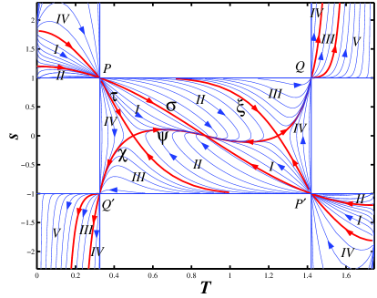
Figure 1: Phase portrait evolution for $k>0$ ($k=0.44$).

The trajectories of class IV begin in the left upper stripe in the point with coordinates $T=0,s=\sqrt{\frac{1+k}{k}}$, which corresponds to the singularity of the standard Big Bang type. These trajectories climb to some maximal value of $s$, then turn down and cross the point $P$, entering the rectangle. Then they leave the rectangle through the point $Q^{\prime}$ entering the left lower stripe. Here, after a finite period of time the universe encounters a special type of cosmological singularity, which we call Big Brake. At this singularity, the tachyon field has some finite value, its velocity $s$ tends to $-\infty$, the cosmological radius has a finite value, its first time derivative is equal to zero, while its second time derivative tends to $-\infty$. The trajectories of class I also begin in the point with coordinates $T=0,s=\sqrt{\frac{1+k}{k}}$, however, after entering the rectangle they end their evolution in the de Sitter node. They are separated from the trajectories of class IV by the separatrix $\tau$, which inside the rectangle connects the corner $P$ with the left saddle point. The trajectories of class II are separated from those of class I by the curve $\sigma$, which begins in the point with coordinates $T=0,s=\sqrt{\frac{1+k}{k}}$, passes through the corner $P$ and ends in the de Sitter node. These trajectories begin at the singularity $s=1,T=T_{in}$, where $0<T_{in}<T_{\ast},\ T_{\ast}>T_{3}$ and end in the de Sitter node. The separatrix $\xi$, ending in the right saddle, separates the trajectories of class II from those of class III. The latter, beginning at $s=1$ and $T=T_{in}$, where $T_{\ast}<T_{in}<T_{4}$, after crossing the corner $Q$ encounter their Big Brake singularity in the upper right infinite stripe. These trajectories are separated from those of class IV by the curve $\chi$, which passes through the right saddle point and the corner $Q$. Finally, the trajectories of the last class V begin at $s=1,T=T_{in}>T_{4}$ and end in the Big Brake singularity. The time dependence of the Hubble parameter for these five classes is represented in Fig. 2.

Figure 2: Time evolution of the Hubble parameter $H(t)$.

We conclude this section by giving some additional formulae characterizing the different types of singularities present in the cosmological model under consideration. In the vicinity of the singularity which takes place at the horizontal sides of the rectangle (say, at $s=1$), we have the following dependence of the function $s$ on $T$ we-tach :

$$s=1-C(T_{in})(T-T_{in})^{4},$$ (14)

where

$$C(T_{in})=\frac{81}{32}\frac{\Lambda^{2}\left(1-(1+k)\cos^{2}\frac{3\sqrt{\Lambda(1+k)}T_{in}}{2}\right)}{\sin^{4}\frac{3\sqrt{\Lambda(1+k)}T_{in}}{2}}.$$ (15)

Hence the energy density is

$$\varepsilon=\frac{V(T_{in})}{\sqrt{2C(T_{in}}(T-T_{in})^{2}}=\frac{4}{9(T-T_{in})^{2}}.$$ (16)

In the vicinity of the singularity $T-T_{in}=t$ and

$$\varepsilon=\frac{4}{9t^{2}}$$ (17)

while the Hubble variable is

$$H=\frac{2}{3t},$$ (18)

just like in the dust-filled universe born in the vicinity of the Big Bang singularity.

For the universe born in the point $s=\sqrt{\frac{1+k}{k}},T=0$ the potential $W$ behaves as

$$W(T)=\frac{4\sqrt{k}}{9(1+k)T^{2}},$$ (19)

where $T=\sqrt{\frac{1+k}{k}}t$. The energy density behaves as

$$\varepsilon=\frac{4k^{2}}{9(1+k)^{2}t^{2}},$$ (20)

while the Hubble variable is

$$H=\frac{2k}{3(1+k)t}.$$ (21)

Thus, one can note that the universe has at this point a Big Bang singularity and behaves in such a way as if it were filled with a perfect barotropic fluid with equation of state parameter $w=\frac{1}{k}$.

We can also describe the behavior of the universe in the vicinity of the final Big Brake singularity following the logic of paper we-tach . Consider the universe which is approaching the Big Brake in the lower left stripe at some value of the tachyon field $T_{BB}$. Correspondingly, the variable $s$ approaches $-\infty$. Analyzing Eq. (5) in this limit we have

$$|s|=\left(\frac{4}{81W(T_{BB})}\right)^{1/3}(t_{BB}-t)^{-2/3},$$ (22)

where $t_{BB}$ means the moment of Big Brake. Now, using the formula (6) and the energy density from (13), one easily finds

$$H=\left(\frac{9W^{2}(T_{BB})}{2}\right)^{1/3}(t_{BB}-t)^{1/3}.$$ (23)

Thus, we see that when $t\rightarrow t_{BB}$, the Hubble variable $H$ vanishes while its time derivative diverges, tending to $-\infty$. It is important to emphasize that the value $T_{BB}$ is rigorously positive $T_{BB}>0$ we-tach .

3 Confrontation with type Ia supernovae

Following Ref. DicusRepko , in Ref. tachyon-prd we have presented in detail how to perform a $\chi^{2}$-test for comparing the prediction of the model with the available type Ia supernovae taken from Ref. SN2007 . In order to do this, we introduce more suitable dimensionless variables

$$\hat{H}=\frac{H}{H_{0}},\,\hat{V}=\frac{V}{H_{0}^{2}},\,\Omega_{\Lambda}=\frac{\Lambda}{H_{0}^{2}},\,\hat{T}=H_{0}T,$$ (24)

where $H_{0}$ is the present value of the Hubble parameter. In general, for any variable $f\left(z\right)$ we will denote by $f_{0}=f(z=0)$. As a follow-up, we also introduce a new tachyonic variable

$$y=\cos\left(\frac{3}{2}\sqrt{\Omega_{\Lambda}(1+k)}\hat{T}\right),$$ (25)

and switch from the time derivative to the derivative with respect to the redshift $z$ by

$$\frac{d}{dt}=-H(1+z)\frac{d}{dz}.$$ (26)

Then we rewrite the equations (6), (4), (5) in terms of the new variables $\hat{H},~{}s,~{}y$ and perform the $\chi^{2}$-test. For this we employ

$$\frac{d}{dz}\left(\frac{\hat{d}_{L}}{1+z}\right)=\frac{1}{\hat{H}}\ ,$$ (27)

where $\hat{d}_{L}=H_{0}d_{L}$ and $d_{L}$ is the luminosity distance for a flat Friedmann universe:

$$d_{L}\left(z\right)=\left(1+z\right)\int_{0}^{z}\frac{dz^{\ast}}{H\left(z^{\ast}\right)}\$$ (28)

The results are represented on the figure panel 3

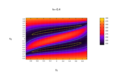
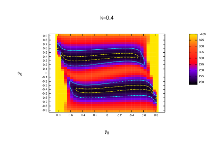
Figure 3: The fit of the luminosity distance vs. redshift for $k=-0.4$ (left) and $0.4$ (right). The white areas represent forbidden parameter regions where the tachyonic field would be superluminal today. The contours refer to the $68.3\%$ (1$\sigma$) and $95.4\%$ (2$\sigma$) confidence levels. For increasing values of $\left|k\right|<1$  the well-fitting regions are increasingly smaller tachyon-prd . The colour code for $\chi^{2}$ is indicated on the vertical stripes. The model is symmetric under the simultaneous change of signs $y_{0}\to-y_{0}$ and $s_{0}\to-s_{0}$, thus there is a double coverage of the parameter space.

4 Future evolution

In order to avoid the double coverage of the parameter space; also to bring the Big Brake at $s\rightarrow\pm\infty$ to finite parameter distance, we introduce the new variable

$$w=\frac{1}{1+s^{2}}~{}.$$ (29)

We do this by numerical integration of equations of motion from $z=0$ towards negative values of $z$. We represent the future evolution for $k=\pm 0.4$ on Fig 4. The evolution curves start from the allowed region ($w_{0},y_{0}$) in the plane $z=0$. The final de Sitter state is characterized by the point ($w_{dS}=1,y_{dS}=0,z_{dS}=-1$), the Big Brake final state by points ($w_{BB}=0,-1<y_{BB}<0,-1<z_{BB}<0$).

Whereas all trajectories with $k=-0.4$ end up eventually into the de Sitter state, those with $k=0.4$ can either evolve into the de Sitter state or into the Big Brake state, depending on the particular initial condition ($w_{0},y_{0}$). These are generic features holding for negative and positive values of $k$, respectively. In Ref. tachyon-prd we have also found, that future evolutions towards the Big Brake singularity of the universes selected by the comparison with supernovae data become more frequent with increasing (positive) $k$.

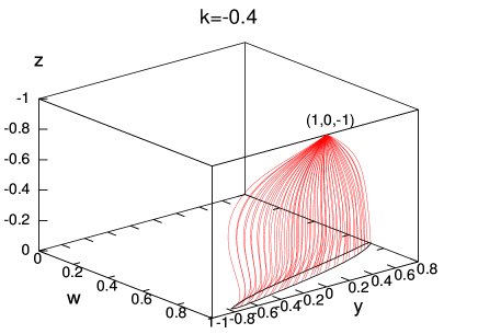
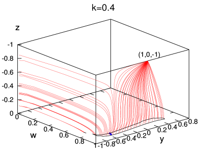
Figure 4: The future evolution of those universes, which are in a $68.3\%$ confidence level fit with the supernova data. The 1$\sigma$ contours (black lines in the $z=0$ plane) are from Fig 3 (the parameter plane $\left(y_{0},w_{0}\right)$ is the $z=0$ plane here). The figures are for $k=-0.4$ (left) and $k=0.4$ (right). The coordinate $w$ is related to the tachyonic speed as $w=1/\left(1+s^{2}\right)$). In the $k=0.4$ case from the 1$\sigma$ parameter range the universe evolves either into a de Sitter regime or towards the Big Brake singularity.

For all future evolutions encountering a Big Brake singularity we have computed the actual time $t_{BB}$ it will take to reach the singularity, measured from the present moment $z=0$, using the equation $\left(H_{0}t\right)^{\prime}=-\hat{H}^{-1}\left(1+z\right)^{-1}$). The results are shown in Table 1. The parameter values at which the pressure turns from negative to positive (at the superluminal crossing) are also displayed.

Table 1: Properties of the tachyonic universes with $k=0.4$ which (a) are within 1$\sigma$ confidence level fit with the type Ia supernova data and (b) evolve into a Big Brake singularity. Columns (1) and (2) represent a grid of values of the allowed model parameters. Columns (3) and (4): the redshift $z_{\ast}$ and time $t_{\ast}$ at the future tachyonic crossing (when $s=1$ and the pressure becomes positive). Columns (5) and (6): the redshift $z_{BB}$ and time $t_{BB}$ necessary to reach the Big Brake. The former indicates the relative size of the universe when it encounters the Big Brake. (The values of $t_{\ast}$ and $t_{BB}$ were computed with the Hubble parameter $H_{0}=73$ km/s/Mpc.)

$y_{0}$ $w_{0}$ $z_{\ast}$ $t_{\ast}\left(10^{9}yrs\right)$ $z_{BB}$ $t_{BB}\left(10^{9}yrs\right)$ $-0.80$ $0.710$ $-0.059$ $0.8$ $-0.106$ $1.6$ $-0.80$ $0.725$ $-0.059$ $0.8$ $-0.105$ $1.6$ $-0.80$ $0.740$ $-0.060$ $0.8$ $-0.105$ $1.6$ $-0.75$ $0.815$ $-0.144$ $2.1$ $-0.184$ $2.9$ $-0.75$ $0.830$ $-0.147$ $2.2$ $-0.187$ $3.0$ $-0.75$ $0.845$ $-0.150$ $2.2$ $-0.189$ $3.0$ $-0.70$ $0.845$ $-0.241$ $3.8$ $-0.276$ $4.6$ $-0.70$ $0.860$ $-0.248$ $4.0$ $-0.282$ $4.7$ $-0.70$ $0.875$ $-0.256$ $4.1$ $-0.290$ $4.9$ $-0.70$ $0.890$ $-0.264$ $4.2$ $-0.298$ $5.0$ $-0.65$ $0.860$ $-0.358$ $6.2$ $-0.387$ $7.0$ $-0.65$ $0.875$ $-0.372$ $6.5$ $-0.400$ $7.2$ $-0.65$ $0.890$ $-0.388$ $6.8$ $-0.415$ $7.6$ $-0.65$ $0.905$ $-0.406$ $7.2$ $-0.432$ $8.0$ $-0.60$ $0.875$ $-0.521$ $10$ $-0.542$ $11$ $-0.60$ $0.890$ $-0.551$ $11$ $-0.571$ $12$ $-0.60$ $0.905$ $-0.587$ $12$ $-0.605$ $13$ $-0.55$ $0.875$ $-0.756$ $19$ $-0.766$ $20$ $-0.55$ $0.890$ $-0.837$ $25$ $-0.845$ $26$

In Ref. tachyon-prd we have also shown that the Big Brake final fate becomes increasingly likely with the increase of the positive model parameter $k$.

References

- (1) A. Riess et al., Astron. J. 116, 1009 (1998); S.J. Perlmutter et al., Astroph. J. 517, 565 (1999).
- (2) V. Sahni and A.A. Starobinsky, Int. J. Mod. Phys. D 9, 373 (2000); 15, 2105 (2006); T. Padmanabhan, Phys. Rep. 380, 235 (2003); P.J.E. Peebles and B. Ratra, Rev. Mod. Phys. 75, 559 (2003); E.J. Copeland, M. Sami, and S.Tsujikawa, Int. J. Mod. Phys. D 15, 1753 (2006).
- (3) A. Y. Kamenshchik, U. Moschella, and V. Pasquier, Phys. Lett. B 511, 265 (2001); M. Bouhmadi-Lopez and P. V. Moniz, Phys. Rev. D 71, 063521 (2005); M. K. Mak and T. Harko, Phys. Rev. D 71, 104022 (2005); C. S. J. Pun, L. Á. Gergely, M. K. Mak, Z. Kovács, G. M. Szabó, and T. Harko, Phys. Rev. D 77, 063528 (2008).
- (4) C. Armendariz-Picon, V. F. Mukhanov, and P. J. Steinhardt, Phys. Rev. D 63, 103510 (2001).
- (5) A. Sen, JHEP 0207, 065 (2002); G.W. Gibbons, Phys. Lett. B 537, 1 (2002); A. Feinstein, Phys. Rev. D 66, 063511 (2002); T. Padmanabhan, Phys. Rev. D 66, 021301 (2002); A. Frolov, L. Kofman, and A. Starobinsky, Phys. Lett. B 545, 8 (2002).
- (6) A. Sen, JHEP 0204, 048 (2002).
- (7) V. Gorini, A.Yu. Kamenshchik, U. Moschella, and V. Pasquier, Phys. Rev. D 69, 123512 (2004).
- (8) J. D. Barrow, G. J. Galloway, and F. J. Tipler, Mon. Not. Roy. Astron. Soc. 223, 835- 844 (1986); J. D. Barrow Phys. Lett. B 235, 40-43 (1990); J. D. Barrow, Class. Quant. Grav. 21, L79 (2004); J. D. Barrow, Class. Quant. Grav. 21, 5619 (2004); J. D. Barrow, A. B. Batista, J. C. Fabris, and S. Houndjo, Phys. Rev. D 78, 123508 (2008).
- (9) M. P. Dabrowski, T. Denkiewicz, and M. A. Hendry, Phys. Rev. D 75, 123524 (2007).
- (10) J. D. Barrow and S. Z. W. Lip, Phys. Rev. D 80, 043518 (2009).
- (11) A. Kamenshchik, C. Kiefer, and B. Sandhöfer, Phys. Rev. D 76, 064032 (2007).
- (12) Z. Keresztes, L. Á. Gergely, A.Yu. Kamenshchik, V. Gorini, and U. Moschella, Phys. Rev. D 79, 083504 (2009).
- (13) Y. Shtanov and V. Sahni, Class. Quant. Grav. 19, L101 (2002).
- (14) A.A. Starobinsky, Grav. Cosmol. 6, 157 (2000); R.R. Caldwell, M. Kamionkowski, and N.N. Weinberg, Phys. Rev. Lett. 91, 071301 (2003).
- (15) R.R. Caldwell, Phys. Lett. B 545, 23 (2002); M. P. Dabrowski, T. Stachowiak, and M. Szydlowski, Phys. Rev. D 68, 103519 (2003); M. P. Dabrowski and T. Stachowiak, Annals Phys. 321, 771-812 (2006); M. P. Dabrowski, C. Kiefer, and B. Sandhöfer, Phys. Rev. D 74, 044022 (2006).
- (16) R. Kallosh, A. Linde, S. Prokushkin, and M. Shmakova, Phys. Rev. D 66, 123503 (2002), R. Kallosh and A. Linde, JCAP 0302, 002 (2003), U. Alam, V. Sahni, and A. A. Starobinsky, JCAP 0304, 002 (2003), R. Kallosh, J. Kratochvil, A. Linde, E. V. Linder, and M. Shmakova, JCAP 0310, 015 (2003).
- (17) W. M. Wood-Vasey et al. [ESSENCE Collaboration], Astrophys. J. 666, 694 (2007).
- (18) D. A. Dicus and W. W. Repko, Phys. Rev. D 70 083527 (2004).