Short-time vs. long-time dynamics of entanglement in quantum lattice models

Abstract

We study the short-time evolution of the bipartite entanglement in quantum lattice systems with local interactions in terms of the purity of the reduced density matrix. A lower bound for the purity is derived in terms of the eigenvalue spread of the interaction Hamiltonian between the partitions. Starting from an initially separable state the purity decreases as $1-(t/\tau)^{2}$, i.e. quadratically in time, with a characteristic time scale $\tau$ that is inversely proportional to the boundary size of the subsystem, i.e., as an area–law. For larger times an exponential lower bound is derived corresponding to the well-known linear-in-time bound of the entanglement entropy. The validity of the derived lower bound is illustrated by comparison to the exact dynamics of a 1D spin lattice system as well as a pair of coupled spin ladders obtained from numerical simulations.

I – Introduction

Motivated by the question whether the time evolution of interacting quantum systems can be efficiently simulated with the help of matrix-product decompositions of the many-body wave function Verstraete et al. (2008); Vidal (2003, 2004) or corresponding analogues in higher dimensions Nishino and Okunishi (1998); Verstraete and Cirac (2004); Murg et al. (2007); Vidal (2007); Verstraete et al. (2008); Sierra and Martin-Delgado (1998), the dynamics of entanglement in quantum lattice models has become an important research area in quantum physics. A convenient measure of entanglement are Schuch et al. (2008) the von Neumann and Rényi entropies. It was shown in Bravyi et al. (2006) and Eisert and Osborne (2006) that the von Neumann entropy of a subsystem which starts in an initially separable state has an upper bound that grows linear in time. The linear growth of the entropy, as observed by Calabrese and co-workers Calabrese and Cardy (2005); Fagotti and Calabrese (2008), which corresponds to an exponential growth of the effective bond dimension of matrix–product states (MPS) represents a severe limitation for the simulability of the unitary time evolution of quantum many-body systems. In the present note we derive an upper bound to the bipartite entanglement that also holds for short times. In particular we consider the purity of the reduced density matrix of one of the partitions. General quantum mechanical arguments suggest that the purity cannot decease exponentially for short times as implied by the linear entanglement bound Lieb and Robinson (1972); Bravyi et al. (2006); Eisert and Osborne (2006), but rather quadratically. Here we derive a quadratic lower bound for the purity. This finding which is the main result of our paper has practical relevance for the numerical simulation of another class of dynamical problems that gained a lot of interest recently where the time evolution is non-unitary due to a coupling to external reservoirs Syassen et al. (2008); Dürr et al. (2009); Garcia-Ripoll et al. (2009); Prosen (2008); Prosen and Pizorn (2008); Prosen and Znidaric (2009); Diehl et al. (2008); Daley et al. (2009); Han et al. (2009); Kantian et al. (2009); Kiffner and Hartmann (2009). The non-unitary Liouvillian dynamics of the system density matrix is equivalent to a time evolution of the many-body wave function with a complex Hamiltonian and with a stochastic sequence of projections, called quantum jumps Carmichael (1993); Dalibard et al. (1992); Mølmer et al. (1993). If the frequency of such projections is sufficiently large they can prevent the growth of entanglement within the system by a mechanism similar to the well-known quantum Zeno effect Facchio and Pascazio (2001). As a result of this the time evolution of open system may be simulated using an adaptive MPS expansion as e.g. within the time evolving block decimation algorithm (TEBD) Vidal (2003, 2004) for longer times. The critical frequency of such a Zeno effect for entanglement is determined by the coefficient of the quadratic term in the short time expansion of the purity. Note that this effect would be absent for an exponential time dependence of the purity. For larger times we derive an exponential lower bound corresponding to the well-known linear–in–time bound of the entanglement entropy Lieb and Robinson (1972); Bravyi et al. (2006); Eisert and Osborne (2006). Although this result follows directly from the latter entropy bound, we derive it here in a few lines without making use of the somewhat more involved proof of the linear entropy scaling. To illustrate the validity of our findings we discuss as an example the 1D spin-$\frac{1}{2}$ XX and XXZ models, where we calculate the time evolution of the purity using the numerical time-evolving block decimation algorithm Vidal (2003, 2004), as well as two coupled spin chains, which allow us to illustrate the scaling with the boundary size.

II – Short-time behavior

We here consider a lattice model with a bipartition into parts $A$ and $B$, which are, say, compact sets of lattice sites. We assume that the Hamiltonian of the total systems can be written as

$$\hat{H}_{AB}=\hat{H}_{A}+\hat{H}_{B}+\sum_{q\in\{A|B\}}\hat{H}_{q}^{\left(A\right)}\otimes\hat{H}_{q}^{\left(B\right)},$$ (1)

where $\hat{H}_{A}$ and $\hat{H}_{B}$ are the parts of the Hamiltonian acting on lattice sites inside the respective partitions. The last sum describes the interaction between the two parts an extends over all bonds, labeled by the index $q$, that connect sites from both partitions. We assume an interaction that has strict finite range. In this case the total number of bonds scales with the size $N$ of the surface separating the two partitions.

Any pure state of the total system can be decomposed as

$$\left|\Psi\left(t\right)\right\rangle_{AB}={\displaystyle\sum\limits_{\alpha=1}^{L}}\sqrt{\xi_{\alpha}}\left|\phi_{\alpha}^{\left(A\right)}\right\rangle\otimes\left|\phi_{\alpha}^{\left(B\right)}\right\rangle,$$ (2)

where $\left|\phi_{\alpha}^{\left(A\right)}\right\rangle$ and $\left|\phi_{\alpha}^{\left(B\right)}\right\rangle$ are orthonormal sets of states of the subsystems, $\xi_{\alpha}\geq 0$ are the Schmidt coefficients, and $L$ is at most the dimension of the Hilbert space of the smaller subsystem. As $\left|\Psi\left(t\right)\right\rangle_{AB}$ is normalized, $\sum\limits_{\alpha}\xi_{\alpha}=1$. The reduced density operator of the subsystem $A$, $\rho_{A}=\mathrm{tr}_{B}\{\rho_{AB}\}$, where $\rho_{AB}=\left|\Psi\left(t\right)\right\rangle_{AB}\left\langle\Psi\left(t\right)\right|_{AB}$, satisfies the equation of motion

$$\frac{\mathrm{d}\rho_{A}}{\mathrm{d}t}=-i\,\mathrm{tr}_{B}\Bigl{\{}\left[\hat{H}_{AB},\rho_{AB}\right]\Bigr{\}}.$$ (3)

(Note that we have set $\hbar=1$ throughout this text.) The form of the Hamiltonian (1) and the cyclic property of the trace allows us to obtain the following equation

$$\frac{\mathrm{d}}{\mathrm{d}t}\mathrm{tr}\rho_{A}^{2}=-2i\mathrm{tr}\left\{\rho_{A}\mathrm{tr}_{B}\left[\sum_{q}\hat{H}_{q}^{\left(A\right)}\otimes\hat{H}_{q}^{\left(B\right)},\rho_{AB}\right]\right\}$$ (4)

for the purity rate. The traces on the right hand side can be calculated in the eigenbasis of the $\rho_{A}$ and $\rho_{B}$:

$$\mathrm{tr}\left\{\rho_{A}\mathrm{tr}_{B}\left(\sum_{q}\hat{H}_{q}^{\left(A\right)}\otimes\hat{H}_{q}^{\left(B\right)}\cdot\rho_{AB}\right)\right\}=\sum\limits_{q,\alpha}\xi_{\alpha}\left\langle\phi_{\alpha}^{\left(A\right)}\right|\mathrm{tr}_{B}\hat{H}_{q}^{\left(A\right)}\otimes\hat{H}_{q}^{\left(B\right)}\rho_{AB}\left|\phi_{\alpha}^{\left(A\right)}\right\rangle=$$ (5)

$$\sum\limits_{q,\alpha,\alpha^{\prime}}\xi_{\alpha}\sqrt{\xi_{\alpha}\xi_{\alpha^{\prime}}}\left\langle\phi_{\alpha}^{\left(A\right)}\right|\mathrm{tr}_{B}\hat{H}_{q}^{\left(A\right)}\otimes\hat{H}_{q}^{\left(B\right)}\left|\phi_{\alpha^{\prime}}^{\left(A\right)}\right\rangle\otimes\left|\phi_{\alpha^{\prime}}^{\left(B\right)}\right\rangle\left\langle\phi_{\alpha}^{\left(B\right)}\right|=$$

$$=\sum\limits_{q,\alpha,\alpha^{\prime}}\xi_{\alpha}\sqrt{\xi_{\alpha}\xi_{\alpha^{\prime}}}\left\langle\phi_{\alpha}^{\left(A\right)}\right|\hat{H}_{q}^{\left(A\right)}\left|\phi_{\alpha^{\prime}}^{\left(A\right)}\right\rangle\mathrm{tr}_{B}\left(\hat{H}_{q}^{\left(B\right)}\left|\phi_{\alpha^{\prime}}^{\left(B\right)}\right\rangle\left\langle\phi_{\alpha}^{\left(B\right)}\right|\right)=$$

$$=\sum\limits_{q,\alpha,\alpha^{\prime}}\xi_{\alpha}\sqrt{\xi_{\alpha}\xi_{\alpha^{\prime}}}\left\langle\phi_{\alpha}^{\left(A\right)}\right|\hat{H}_{q}^{\left(A\right)}\left|\phi_{\alpha^{\prime}}^{\left(A\right)}\right\rangle\left\langle\phi_{\alpha}^{\left(B\right)}\right|\hat{H}_{q}^{\left(B\right)}\left|\phi_{\alpha^{\prime}}^{\left(B\right)}\right\rangle,$$ (6)

and in the same way, the second term of the commutator is

$$\mathrm{tr}\left\{\rho_{A}\mathrm{tr}_{B}\left(\rho_{AB}\cdot\sum_{q}\hat{H}_{q}^{\left(A\right)}\otimes\hat{H}_{q}^{\left(B\right)}\right)\right\}=\sum\limits_{q,\alpha,\alpha^{\prime\prime}}\xi_{\alpha}\sqrt{\xi_{\alpha}\xi_{\alpha^{\prime\prime}}}\left\langle\phi_{\alpha^{\prime\prime}}^{\left(A\right)}\right|\hat{H}_{q}^{\left(A\right)}\left|\phi_{\alpha}^{\left(A\right)}\right\rangle\left\langle\phi_{\alpha^{\prime\prime}}^{\left(B\right)}\right|\hat{H}_{q}^{\left(B\right)}\left|\phi_{\alpha}^{\left(B\right)}\right\rangle.$$ (7)

Combining eqs. (4), (6) and (7) one obtains the following differential equation for the purity

$$\frac{\mathrm{d}}{\mathrm{d}t}\mathrm{tr}\rho_{A}^{2}=-2i\sum\limits_{q,\alpha,\beta}\sqrt{\xi_{\alpha}\xi_{\beta}}\left(\xi_{\alpha}-\xi_{\beta}\right)\times$$ (8)

$$\quad\times\left\langle\phi_{\alpha}^{\left(A\right)}\right|\hat{H}_{q}^{\left(A\right)}\left|\phi_{\beta}^{\left(A\right)}\right\rangle\left\langle\phi_{\alpha}^{\left(B\right)}\right|\hat{H}_{q}^{\left(B\right)}\left|\phi_{\beta}^{\left(B\right)}\right\rangle.$$

This equation can be rewritten in a compact form

$$\frac{\mathrm{d}}{\mathrm{d}t}\mathrm{tr}\rho_{A}^{2}=\mathrm{tr}\left[\Theta\cdot Q\right],$$ (9)

where

$$\Theta_{\alpha\beta}=-2i\sqrt{\xi_{\alpha}\xi_{\beta}}\left(\xi_{\alpha}-\xi_{\beta}\right)$$ (10)

and

$$Q_{\alpha\beta}=\sum\limits_{q}\left\langle\phi_{\alpha}^{\left(A\right)}\right|\hat{H}_{q}^{\left(A\right)}\left|\phi_{\beta}^{\left(A\right)}\right\rangle\left\langle\phi_{\alpha}^{\left(B\right)}\right|\hat{H}_{q}^{\left(B\right)}\left|\phi_{\beta}^{\left(B\right)}\right\rangle$$ (11)

The matrix $\Theta$ has only two non-zero eigenvalues. Indeed, $\Theta$ can be written as

$$\Theta=-2i\left|a\right\rangle\left\langle b\right|+2i\left|b\right\rangle\left\langle a\right|,$$ (12)

where

$$\left|a\right\rangle =\left(\xi_{1}^{3/2},\xi_{2}^{3/2},\dots\xi_{L}^{3/2}\right)^{T},$$

$$\left|b\right\rangle =\left(\xi_{1}^{1/2},\xi_{2}^{1/2},\dots\xi_{L}^{1/2}\right)^{T}.$$

It is easy to show that the nonzero eigenvalues of $\Theta$ are

$$\lambda_{\pm}\left(\Theta\right) = \pm 2\sqrt{\left\langle a\right.\left|a\right\rangle\left\langle b\right|\left.b\right\rangle-\left|\left\langle a\right|\left.b\right\rangle\right|^{2}}$$

$$= \pm 2\sqrt{\mathrm{tr}\rho_{A}^{3}-\left(\mathrm{tr}\rho_{A}^{2}\right)^{2}}.$$

Let $\left|q_{\pm}\right\rangle$ be the corresponding eigenvectors of $\Theta$, then the trace (9) can be evaluated in the eigenbasis of $\Theta$ which yields the following equation for the purity rate

$$\frac{\mathrm{d}}{\mathrm{d}t}\mathrm{tr}\rho_{A}^{2}=2\sqrt{\mathrm{tr}\rho_{A}^{3}-\left(\mathrm{tr}\rho_{A}^{2}\right)^{2}}\Bigl{(}\left\langle q_{+}\right|Q\left|q_{+}\right\rangle-\left\langle q_{-}\right|Q\left|q_{-}\right\rangle\Bigr{)}.$$ (14)

The right side of this equation can be bounded from above by the spread of the eigenvalues of the interaction Hamiltonian between partitions $A$ and $B$:

$$\frac{\mathrm{d}}{\mathrm{d}t}\mathrm{tr}\rho_{A}^{2}\leq 2\sqrt{\mathrm{tr}\rho_{A}^{3}-\left(\mathrm{tr}\rho_{A}^{2}\right)^{2}}\Bigl{[}\lambda_{\max}-\lambda_{\min}\Bigr{]}$$ (15)

Here $\lambda_{\max}$ and $\lambda_{\min}$ are the maximum and minimum eigenvalues of $\sum_{q\in\{A|B\}}\hat{H}_{q}^{(A)}\otimes\hat{H}_{q}^{(B)}$.

In a similar way one can show that

$$\frac{\mathrm{d}}{\mathrm{d}t}\mathrm{tr}\rho_{A}^{2}\geq-2\sqrt{\mathrm{tr}\rho_{A}^{3}-\left(\mathrm{tr}\rho_{A}^{2}\right)^{2}}\Bigl{[}\lambda_{\max}-\lambda_{\min}\Bigr{]}.$$ (16)

Combining the inequalities (15) and (16) we obtain

$$\left|\frac{\mathrm{d}}{\mathrm{d}t}\mathrm{tr}\rho_{A}^{2}\right|\leq 2\mu\sqrt{\mathrm{tr}\rho_{A}^{3}-\left(\mathrm{tr}\rho_{A}^{2}\right)^{2}},$$ (17)

where

$$\mu=\lambda_{\max}\left(\sum_{q}\hat{H}_{q}^{(A)}\otimes\hat{H}_{q}^{(B)}\right)-\lambda_{\min}\left(\sum_{q}\hat{H}_{q}^{(A)}\otimes\hat{H}_{q}^{(B)}\right)$$

is a constant that scales linear with the size $N$ of the surface separating the subsystems.

In order to solve the differential inequality (17) we need an expression or at least an estimate for $\mathrm{tr}\rho_{A}^{3}$ in terms of the purity. With the help of Hardy’s inequality $\left(\sum_{k}a_{k}^{m}\right)^{1/m}\leq\left(\sum_{k}a_{k}^{n}\right)^{1/n}$ for any $a_{k}\geq 0$, and $m>n>0$, (see Hardy et al. (1952)), one can show that $\mathrm{tr}\rho_{A}^{3}\leq\left(\mathrm{tr}\rho_{A}^{2}\right)^{3/2}$. With this we find the following differential inequality for the purity

$$\left|\frac{\mathrm{d}}{\mathrm{d}t}\mathrm{tr}\rho_{A}^{2}\right|\leq 2\mu\sqrt{\left(\mathrm{tr}\rho_{A}^{2}\right)^{3/2}-\left(\mathrm{tr}\rho_{A}^{2}\right)^{2}}.$$ (18)

In general the short time behavior is local, and eq. (18) partially supports this intuition, since the control parameter is $\mu$, the spread of the local Hamiltonian. However, due to the second factor the dynamics of the purity does not only depend on the local Hamiltonian, but also on the purity of the initial state (see examples).

We can divide the left- and right-hand side by the square root term, which after integration yields

$$\left|\frac{\mathrm{d}}{\mathrm{d}t}\arcsin\left(\left(\mathrm{tr}\rho_{A}^{2}\right)^{1/4}\right)\right|\leq\frac{\mu}{2}.$$ (19)

Using

$$\arcsin\left[\left(\mathrm{tr}\rho_{A}^{2}\right)^{1/4}\right] = \int\limits_{0}^{t}\frac{\mathrm{d}}{\mathrm{d}\tau}\Bigl{[}\arcsin\left(\left(\mathrm{tr}\rho_{A}^{2}\right)^{1/4}\right)\Bigr{]}\mathrm{d}\tau+$$ (20)

$$+\arcsin\left(\left(\mathrm{tr}\rho_{A}^{2}\left(0\right)\right)^{1/4}\right)$$

gives a solution of eq.(18) with the initial purity $\mathrm{tr}\rho_{A}^{2}\left(0\right)$

$$\sin^{4}\left[\max\left(-\frac{\mu}{2}t+\arcsin\left(\mathrm{tr}\rho_{A}^{2}\left(0\right)\right)^{1/4},0\right)\right]\leq\mathrm{tr}\rho_{A}^{2}$$

$$\enspace\leq\sin^{4}\left[\min\left(\frac{\mu}{2}t+\arcsin\left(\mathrm{tr}\rho_{A}^{2}\left(0\right)\right)^{1/4},\frac{\pi}{2}\right)\right].$$ (21)

If $\mathrm{tr}\rho_{A}^{2}\left(0\right)=1$, i.e. if the subsystems are uncorrelated in the beginning, the upper bound is trivial. The lower bound reduces to

$$\mathrm{tr}\rho_{A}^{2}\geq\cos^{4}\frac{\mu t}{2},\qquad\text{for}\enspace\mu t\leq\pi.$$ (22)

We note that the lower bound becomes zero at $\mu t>\pi$ i.e. it reduces to the trivial one.

The lower bound can be slightly improved, if we know the maximum Schmidt rank $L_{\mathrm{max}}$ of the bipartite decomposition that can arise along the evolution. One finds

$$\mathrm{tr}\rho_{A}^{2}\geq\cos^{4}\frac{\mu t}{2}+\frac{1}{L_{\mathrm{max}}-1}\sin^{4}\frac{\mu t}{2}.$$ (23)

Evidently $\mathrm{tr}\rho_{A}^{2}\geq L_{\mathrm{max}}^{-1}$ as it should be. Typically $L_{\mathrm{max}}\gg 1$ and thus the second term in eq.(23) is small. In the general case, $L_{\mathrm{max}}$ can be the dimension of the smaller Hilbert space. So one must assume this, if there is no better bound known a priori. In certain special cases as for the 1D quantum Ising model with an initial state that factorizes in all sites, $L_{\mathrm{max}}=2$, and the lower bound (23) becomes exact, see below.

The estimation (23) follows from the inequality

$$tr\rho^{3}\leq\frac{1}{L_{\rm max}^{3}}\left[\left(1+\sqrt{\left(L_{\rm max}-1\right)\left(L_{\rm max}\cdot tr\rho^{2}-1\right)}\right)^{3}+\frac{\left(L_{\rm max}-1-\sqrt{\left(L_{\rm max}-1\right)\left(L_{\rm max}\cdot tr\rho^{2}-1\right)}\right)^{3}}{\left(L_{\rm max}-1\right)^{2}}\right]$$ (24)

which can be proven by the method of Lagrange multipliers.

Eqs. (21) and (22), resp. (23), provide an estimate for the purity for short times. As expected from general quantum mechanical arguments the lower bound of the purity decreases quadratically in time following $\sim-(t/\tau)^{2}$. The characteristic time $\tau$ that defines the range of validity of the quadratic time scaling is inverse proportional to the eigenvalue spread $\mu$ and scales linearly with the size of the surface $N$ separating the subsystems and thus has an area-law behavior. In order to test the scaling of the lower bound with the boundary size of the system we consider next a pair of linear spin chains subject to an Ising interaction

$$\hat{H}=\sum_{j=1}^{N}\hat{\sigma}_{j}^{x}\otimes\hat{\tau}_{j}^{x},$$ (25)

where $\hat{\sigma}$ and $\hat{\tau}$ are the Pauli operators of the two chains respectively. If the initial state is

$$\left|\Downarrow_{A}\Uparrow_{B}\right\rangle=\left|\downarrow\downarrow\dots\downarrow\right\rangle_{A}\otimes\left|\uparrow\uparrow\dots\uparrow\right\rangle_{B}$$ (26)

i.e. where all spins in chain $A$ are in the eigenstate of $\hat{\sigma}^{z}$, resp. $\hat{\tau}^{z}$, with spin down and all spins in chain $B$ in the corresponding spin up state, the purity is given by

$$\text{tr}\rho^{2}=\left(\cos^{4}t+\sin^{4}t\right)^{N}$$ (27)

This can be seen easily, as for the initial product state the total purity can be represented as

$$\text{tr}\rho^{2}=\text{tr}{\prod\limits_{i=1}^{N}}\rho_{i}^{2}=\left(\text{tr}\rho_{1}^{2}\right)^{N}=\left(\cos^{4}t+\sin^{4}t\right)^{N}$$ (28)

because each spin pair of the coupled chains has a purity equal to $\cos^{4}t+\sin^{4}t$. We thus see, that the characteristic time $\tau$ scales as $\sqrt{N}$ for this choice of the initial state. However, if one considers a Greenberger-Horne-Zeilinger type initial state

$$\left|{\rm GHZ}\right\rangle_{A}\otimes\left|{\rm GHZ}\right\rangle_{B}=\left(\frac{1}{\sqrt{2}}\left|++\dots+\right\rangle_{A}+\frac{1}{\sqrt{2}}\left|--\dots-\right\rangle_{A}\right)\otimes\left(\frac{1}{\sqrt{2}}\left|++\dots+\right\rangle_{B}+\frac{1}{\sqrt{2}}\left|--\dots-\right\rangle_{B}\right)$$ (29)

with $|\pm\rangle$ denoting eigenstates of $\hat{\sigma}^{x}$, resp. $\hat{\tau}^{x}$, one finds

$$\text{tr}\rho^{2}=\cos^{4}Nt+\sin^{4}Nt,$$ (30)

as can be shown by simple algebraic calculations. We see that (30) coincides with our estimation (23) since $\mu=2N$ and $L_{\mathrm{max}}=2$. In other words, our estimate is a tight lower bound for the purity. In this case the system size scaling of the characteristic time is $N$.

Note, that in the special case of an Ising Hamiltonian, our two-chains example in fact represents also higher dimensional Ising lattices of arbitrary size. Since all summands in the Ising Hamiltonian, say on a hyper-cubic lattice commute, they can be absorbed in the quantum states of the subsystems $A$ an $B$. They play no role for the entanglement, which is only created by the terms directly coupling $A$ and $B$. But those can always be written in the form (25), no matter what the spacial dimension of the surface is.

For short times, the quadratic estimate (22) is much better than any exponential one (34) (see below). Furthermore it is of fundamental importance. It shows e.g. that a sequence of frequent projections of the system onto non-entangled states (i.e. no entanglement within the system) at a rate larger than $\mu$ will prevent the build-up of such an entanglement in full analogy to the quantum Zeno effect Facchio and Pascazio (2001).

III – Long time behavior

The long time behavior of the purity can be obtained from the known upper linear-in-time bound of the entropy Bravyi et al. (2006); Eisert and Osborne (2006); Lieb and Robinson (1972). Indeed, by using the convexity of $-\ln x,$ we immediately get

$$S=-\sum\limits_{i}\xi_{i}\ln\xi_{i}\geq-\ln\sum\limits_{i}\xi_{i}^{2}=-\ln\mathrm{tr}\rho_{A}^{2},$$ (31)

We thus have

$$\mathrm{tr}\rho_{A}^{2}\geq\exp(-S)\geq\exp\left(-c_{0}\right)\,\exp\left(-c_{1}t\right),$$

where $S\leq c_{0}+c_{1}t$, $c_{0}$ and $c_{1}$ being positive constants.

In the following we show that (31) can also be obtained in a simple way from our approach without the necessity to invoke the rather involved proof of the linear-in-time-bound of the entropy.

In order to find a suitable estimate for the long-time behavior of the purity one has to find a different way to bound the right hand side of eq. (8). The interference effects become negligible at $t\gg\frac{1}{\mu}$ and therefore we may use inequalities of the Schwartz type. In other words, we may sum all interactions (matrix elements) in modulus instead of amplitude. In this case one finds

$$\left|\frac{\mathrm{d}}{\mathrm{d}t}\mathrm{tr}\rho_{A}^{2}\right|\leq 2\sum\limits_{q,\alpha,\beta}\sqrt{\xi_{\alpha}\xi_{\beta}}\left|\xi_{\alpha}-\xi_{\beta}\right|\times\,$$

$$\enspace\times\left|\left\langle\phi_{\alpha}^{\left(A\right)}\right|\hat{H}_{q}^{\left(A\right)}\left|\phi_{\beta}^{\left(A\right)}\right\rangle\left\langle\phi_{\alpha}^{\left(B\right)}\right|\hat{H}_{q}^{\left(B\right)}\left|\phi_{\beta}^{\left(B\right)}\right\rangle\right|$$ (32)

$$\leq\sqrt{2}\sum\limits_{q,\alpha,\beta}\xi_{\alpha}^{2}\left|\left\langle\phi_{\alpha}^{\left(A\right)}\right|\hat{H}_{q}^{\left(A\right)}\left|\phi_{\beta}^{\left(A\right)}\right\rangle\left\langle\phi_{\alpha}^{\left(B\right)}\right|\hat{H}_{q}^{\left(B\right)}\left|\phi_{\beta}^{\left(B\right)}\right\rangle\right|.$$

Here we have used

$$\sqrt{2\xi_{\alpha}\xi_{\beta}}\left|\xi_{\alpha}-\xi_{\beta}\right|\leq\frac{\xi_{\alpha}^{2}+\xi_{\beta}^{2}}{2}.$$

Making use of Schwartz’s inequality, we obtain

$$\sum\limits_{\beta}\left|\left\langle\phi_{\alpha}^{\left(A\right)}\right|\hat{H}_{q}^{\left(A\right)}\left|\phi_{\beta}^{\left(A\right)}\right\rangle\left\langle\phi_{\alpha}^{\left(B\right)}\right|\hat{H}_{q}^{\left(B\right)}\left|\phi_{\beta}^{\left(B\right)}\right\rangle\right|\leq$$

$$\sqrt{\sum\limits_{\beta}\left|\left\langle\phi_{\alpha}^{\left(A\right)}\right|\hat{H}_{q}^{\left(A\right)}\left|\phi_{\beta}^{\left(A\right)}\right\rangle\right|^{2}\sum\limits_{\beta}\left|\left\langle\phi_{\alpha}^{\left(B\right)}\right|\hat{H}_{q}^{\left(B\right)}\left|\phi_{\beta}^{\left(B\right)}\right\rangle\right|^{2}}$$

$$=\sqrt{\left\langle\phi_{\alpha}^{\left(A\right)}\right|\left(\hat{H}_{q}^{\left(A\right)}\right)^{2}\left|\phi_{\alpha}^{\left(A\right)}\right\rangle\left\langle\phi_{\alpha}^{\left(B\right)}\right|\left(\hat{H}_{q}^{\left(B\right)}\right)^{2}\left|\phi_{\alpha}^{\left(B\right)}\right\rangle}$$

$$\leq\sqrt{\lambda_{\max}\left[\left(\hat{H}_{q}^{\left(A\right)}\right)^{2}\right]\lambda_{\max}\left[\left(\hat{H}_{q}^{\left(B\right)}\right)^{2}\right]}.$$

We thus arrive at

$$\left|\frac{\mathrm{d}}{\mathrm{d}t}\mathrm{tr}\rho_{A}^{2}\right|\leq\chi\,\mathrm{tr}\rho_{A}^{2},$$ (33)

where

$$\chi=\sqrt{2}\,\sum\limits_{q}\sqrt{\lambda_{\max}\left[\left(\hat{H}_{q}^{\left(A\right)}\right)^{2}\right]\lambda_{\max}\left[\left(\hat{H}_{q}^{\left(B\right)}\right)^{2}\right]}.$$

The solution of this differential inequality with the initial condition $\mathrm{tr}\rho_{A}^{2}\left(0\right)=1$ is

$$\mathrm{tr}\rho_{A}^{2}\geq\exp\Bigl{(}-\chi t\Bigr{)}.$$ (34)

IV – Numerical examples: spin–$\frac{1}{2}$ XX- and XXZ-chains, multidimensional quantum Ising model

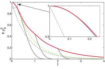
Figure 1: (color online) Time evolution of the purity in the $80+80$ site XX chain compared to the bounds (22) and (34), see text. The inset shows a closeup for short times. Note that $t$ has no units since we have choosen the dimensionless Hamiltonian (35).

To illustrate the quality of the bounds given in (22) and (34) we perform exact numerical simulations for a large 1D spin system as well as for two coupled spin chains of small size. We first consider the spin-$\frac{1}{2}$ XX–model

$$\hat{H}=-\frac{1}{2}\sum_{j}\left(\hat{\sigma}_{j}^{x}\hat{\sigma}_{j+1}^{x}+\hat{\sigma}_{j}^{y}\hat{\sigma}_{j+1}^{y}\right).$$ (35)

For this model the constants which enter our estimates take on the values $\mu=2$ and $\chi=\sqrt{2}$. We look at a chain of $160$ spins and in order to maximize the dimension of the subsystems we choose an equal partition with $A$ ($B$) being the left (right) half chain. The initial state of the system is taken to be a product state, specifically the anti-ferromagnetic state

$$\left|\Psi_{A}(t=0)\right\rangle=\left|\Psi_{B}(t=0)\right\rangle=\left|\uparrow\downarrow\uparrow\downarrow\uparrow\downarrow\cdots\uparrow\downarrow\right\rangle.$$ (36)

We choose this particular initial state in order to have a large maximum entropy since $|\Psi_{A}(t=0)\rangle$ corresponds to half filling, so the dimension of the Hilbert space accessible with respect to the present conservation of the total z–magnetization is maximized. The purity is initially $1$. Fig. 1 shows the evolution of the purity over time. The red, straight, thick line is the numerical results from our simulation using the time-evolving block decimation (TEBD) method Vidal (2003, 2004). This results can be considered numerically exact as discussed below. The solid, black, thinner lines show the bounds (22). The one starting at $t=0$ indicates that our bound is optimal up to second order for times short compared to the inverse coupling between $A$ and $B$, if we start initially from a pure state. However when starting from an initially entangled state, we can only expect to get agreement up to zeroth order from (21), as illustrated by the black, solid, thinner lines starting at $t=1$ and $t=2$. While the exponential lower bound (34), plotted in the dashed line, is bad for short times, it has the property of remaining finite for all times in contrast to (22). So one can smoothly concatenate the two bounds at time

$$t_{1}=\frac{2}{\mu}\arctan\left(\frac{\chi}{2\mu}\right),$$ (37)

assuming we started with a pure state at $t=0$. This combined bound is superior to both the quadratic short-time and exponential long-time estimates and is shown as a green, dot-dashed line.

Analogous calculations where also done for the spin-$\frac{1}{2}$ XXZ–model

$$\hat{H}=-\frac{1}{2}\sum_{j}\left(\hat{\sigma}_{j}^{x}\hat{\sigma}_{j+1}^{x}+\hat{\sigma}_{j}^{y}\hat{\sigma}_{j+1}^{y}+\Delta\hat{\sigma}_{j}^{z}\hat{\sigma}_{j+1}^{z}\right),$$ (38)

choosing the anisotropy $\Delta$ to be $\frac{1}{2}$. This again yields a constant of $\mu=2$ for the short time behavior. But while the exponential bound increases to $\chi=\frac{5}{2\sqrt{2}}$ and one could expect a faster decay of the purity due to the fact that this system can not be mapped to free fermions, the true curves are very much alike for both systems, see Fig. 2.

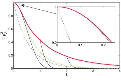
Figure 2: (color online) Time evolution of the purity in the $80+80$ site XXZ chain for $\Delta=\frac{1}{2}$ compared to the bounds (22) and (34) in analogy to Fig. 1. The inset shows a closeup for short times. The dotted lines show the purity in the XX–model (Fig. 1) for comparison.

The numerical calculation was done using a matrix dimension of $D=500$, a time-step width of $0.01$ in a fourth order Trotter decomposition, and exploiting the conservation of the total magnetization explicitly. Although the dimension of the subsystems is adaptively truncated to $D$, this cannot introduce error on the timescale plotted, since the purity remains well above the minimal value of $1/D$ representable using matrix product states. Thus all relevant states are included by the algorithm.

Figure 3 illustrates the tightness of (22) for proper initial conditions. It shows $1-\mathrm{tr}\rho_{A}^{2}$ in a system of two Ising spin chains of length $N$, subject to the Hamiltonian (25), after a short time of $t=0.001$ of evolution. Ising-type couplings inside the chains where also taken into account, but do not contribute to the entanglement between the two chains. While for simple product states between the sites, one can expect a scaling of $\tau\sim\sqrt{N}$ (dashed line), we know from (30), that there are in fact initial states, that contain sufficient entanglement along the boundary, to give$\tau\sim{N}$, i. e., where (22) is tight. The different symbols correspond to different initial states, the evolution of which was calculated via an exact diagonalization. As already seen above, we have a $N$ scaling for an initial product state like (26), while we get an exact $N^{2}$ scaling for GHZ-like initial states (29). Also shown are other states like the W-type states $\left|W_{p}\right\rangle_{A}\otimes\left|W_{p}\right\rangle_{B}$, where

$$\left|W_{p}\right\rangle=\sum_{1\leq j_{1}<j_{2}<\dots<j_{p}\leq N}\hat{\sigma}^{x}_{j_{1}}\hat{\sigma}^{x}_{j_{2}}\dots\hat{\sigma}^{x}_{j_{p}}\left|\downarrow\downarrow\dots\downarrow\right\rangle.$$ (39)

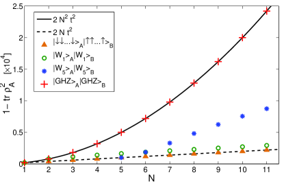
Figure 3: (color online) Short time scaling of the purity with boundary size for a pair of coupled spin chains with Ising interaction. Exact diagonalization was done for $t=0.001$, such that the quadratic order in (22) and (28) suffices to describe the result. While the GHZ-like initial states show the fastest increase of entanglement ($\tau\sim N$, eq. (22), straight line), and the product like ones stick to the moderate $\tau\sim\sqrt{N}$ (eq. (28), dashed line), W-type states show an intermediate behavior.

Summary

In summary we derived an upper bound for the time evolution of the bipartite entanglement in quantum lattice models in terms of a lower bound to the subsystem purity. As one would expect from general quantum mechanical considerations the purity decreases for short times quadratically in time. The corresponding characteristic time was shown to be limited by the spread of the eigenvalues of the part of the Hamiltonian that accounts for the interaction between the partitions. The latter scales linear with the size of the surface separating the two partitions and thus the entanglement follows an area-law behavior. For larger times we derived a lower bound of the purity that decrease exponentially in time. The latter is equivalent to the known linear increase of the entanglement entropy in the long-time limit. The existence of a quadratic short-time bound means that a sufficiently frequent sequence of projections to non-entangled states, as for example due to a dissipative process, can prevent the build-up of entanglement within the lattice system.

References

• Verstraete et al. (2008) F. Verstraete, J. I. Cirac, and V. Murg, Adv. Phys. 57, 143 (2008).
• Vidal (2003) G. Vidal, Physical Review Letters 91, 147902 (2003).
• Vidal (2004) G. Vidal, Physical Review Letters 93, 040502 (2004).
• Nishino and Okunishi (1998) T. Nishino and K. Okunishi, Journal of the Physical Society of Japan 67, 3066 (1998).
• Verstraete and Cirac (2004) F. Verstraete and J. I. Cirac, arXiv:cond-mat/0407066 (2004).
• Murg et al. (2007) V. Murg, F. Verstraete, and J. I. Cirac, Physical Review A 75, 033605 (2007).
• Vidal (2007) G. Vidal, Physical Review Letters 99, 220405 (2007).
• Sierra and Martin-Delgado (1998) G. Sierra and M. A. Martin-Delgado, arXiv:cond-mat/9811170 (1998).
• Schuch et al. (2008) N. Schuch, M. M. Wolf, F. Verstraete, and J. I. Cirac, Physical Review Letters 100, 030504 (2008).
• Bravyi et al. (2006) S. Bravyi, M. B. Hastings, and F. Verstraete, Physical Review Letters 97, 050401 (2006).
• Eisert and Osborne (2006) J. Eisert and T. J. Osborne, Physical Review Letters 97, 150404 (2006).
• Calabrese and Cardy (2005) P. Calabrese and J. Cardy, Journal of Statistical Mechanics-theory and Experiment p. P04010 (2005).
• Fagotti and Calabrese (2008) M. Fagotti and P. Calabrese, Physical Review A 78, 010306(R) (2008).
• Lieb and Robinson (1972) E. H. Lieb and D. W. Robinson, Communications in Mathematical Physics 28, 251 (1972).
• Syassen et al. (2008) N. Syassen, D. M. Bauer, M. Lettner, T. Volz, D. Dietze, J. J. Garcia-Ripoll, J. I. Cirac, G. Rempe, and S. Dürr, Science 320, 1329 (2008).
• Dürr et al. (2009) S. Dürr, J. J. Garcia-Ripoll, N. Syassen, D. M. Bauer, M. Lettner, J. I. Cirac, and G. Rempe, Physical Review A 79, 023614 (2009).
• Garcia-Ripoll et al. (2009) J. J. Garcia-Ripoll, S. Dürr, N. Syassen, D. M. Bauer, M. Lettner, G. Rempe, and J. I. Cirac, New Journal of Physics 11, 013053 (2009).
• Prosen (2008) T. Prosen, New Journal of Physics 10, 043026 (2008).
• Prosen and Pizorn (2008) T. Prosen and I. Pizorn, Physical Review Letters 101, 105701 (2008).
• Prosen and Znidaric (2009) T. Prosen and M. Znidaric, Journal Of Statistical Mechanics-Theory And Experiment 2009, P02035 (2009).
• Diehl et al. (2008) S. Diehl, A. Micheli, A. Kantian, B. Kraus, H. P. Buchler, and P. Zoller, Nature Physics 4, 878 (2008).
• Daley et al. (2009) A. J. Daley, J. M. Taylor, S. Diehl, M. Baranov, and P. Zoller, Physical Review Letters 102, 040402 (2009).
• Han et al. (2009) Y. J. Han, Y. H. Chan, W. Yi, A. J. Daley, S. Diehl, P. Zoller, and L. M. Duan, Physical Review Letters 103, 070404 (2009).
• Kantian et al. (2009) A. Kantian, M. Dalmonte, S. Diehl, W. Hofstetter, P. Zoller, and A. J. Daley, Physical Review Letters 103, 240401 (2009).
• Kiffner and Hartmann (2009) M. Kiffner and M. J. Hartmann, arXiv:0908.2055 (2009).
• Carmichael (1993) H. Carmichael, An open systems approach to quantum optics (Springer, 1993).
• Dalibard et al. (1992) J. Dalibard, Y. Castin, and K. Mølmer, Physical Review Letters 68, 580 (1992).
• Mølmer et al. (1993) K. Mølmer, Y. Castin, and J. Dalibard, Journal of the Optical Society of America B – optical Physics 10, 524 (1993).
• Facchio and Pascazio (2001) P. Facchio and S. Pascazio, Progress in Optics 42, 147 (2001).
• Hardy et al. (1952) G. H. Hardy, J. E. Littlewood, and G. Polya, Inequalities (Cambridge University Press, 1952).