Dynamics and Eccentricity Formation of Planets in OGLE-06-109L System

Abstract

Recent observation of microlensing technique reveals two giant planets at 2.3 AU and 4.6 AU around the star OGLE-06-109L. The eccentricity of the outer planet ($e_{c}$) is estimated to be 0.11${}_{-0.04}^{+0.17}$, comparable to that of Saturn (0.01-0.09). The similarities between the OGLE-06-109L system and the solar system indicate that they may have passed through similar histories during their formation stage. In this paper we investigate the dynamics and formation of the orbital architecture in the OGLE-06-109L system. For the present two planets with their nominal locations, the secular motions are stable as long as their eccentricities ($e_{b},~{}e_{c}$) fulfill $e_{b}^{2}+e_{c}^{2}\leq 0.3^{2}$. Earth-size bodies might be formed and are stable in the habitable zone (0.25AU-0.36AU) of the system. Three possible scenarios may be accounted for formation of $e_{b}$ and $e_{c}$: (i) convergent migration of two planets and the 3:1 MMR trapping; (ii) planetary scattering; (iii) divergent migration and the 3:1 MMR crossing. As we showed that the probability for the two giant planets in 3:1 MMR is low ($\sim 3\%$), scenario (i) is less likely. According to models (ii) and (iii), the final eccentricity of inner planet ($e_{b}$) may oscillate between [0-0.06], comparable to that of Jupiter (0.03-0.06). An inspection of $e_{b}$, $e_{c}$’s secular motion may be helpful to understand which model is really responsible for the eccentricity formation.

1 Introduction

To date, more than 370 exoplanets are detected mainly by Doppler radial velocity measurements(), among them 9 planets are revealed by gravitational microlensing (Udalski et al. 2005; Beaulieu et al. 2006; Bennett et al. 2006, 2008; Gould et al. 2006; Gaudi et al. 2008; Dong et al. 2009; Janczak et al. 2009). The use of microlensing technique to planet-searching is based on the idea of general relativity that light passing through a mass should bend as if it passes a lens (Mao & Paczynski 1991). The major advantage of the technique is that it favors to detect planets in moderate distance to the host star ($\sim$ 3 AU), which is complimentary to the radial velocity measurements. Among the planets detected by microlensing, OGLE-06-109L system is the first one with observed multiple planets. It is 1490 pc away from the Sun, with a star of $\sim 0.5~{}M_{\odot}$ (solar mass) and two planets of $0.71~{}M_{J}$ (Jupiter mass) and 0.27 $M_{J}$ in the orbits of 2.3 AU and 4.6 AU, respectively (Gaudi et al. 2008). Table 1 lists their nominal orbital elements.

Several features of the system make it an analogy of the solar system. (i) The two planets have positions and masses similar to those of Jupiter and Saturn up to scale changes. (ii) The fitted eccentricity of OGLE-06-109L c is modest (0.11${}_{-0.04}^{+0.17}$), comparable with those of Jupiter (0.03-0.06) and Saturn (0.01-0.09) during their secular evolution, although the eccentricity of OGLE-06-109L b is unknown. (iii) While Jupiter and Saturn’s orbits are closing to $5:2$ mean motion resonance (MMR), OGLE-06-109L b and c may be close to $3:1$ MMR. (iv) All these four giant planets are located well outside the snow lines of their systems ($\sim 0.68$ AU for OGLE-06-109L and $\sim 2.7$ AU for solar system), indicating that, unlike the most observed extra-solar systems with hot Jupiters, the migration of these four giant planets were not so efficient. (v) The habitable zone of the OGLE-06-109L system, [0.25AU-0.36AU], may have stable orbits.

Considering most of the observed exoplanets have close-in orbits with an average eccentricity $\sim 0.2$ (Udry & Santos 2007), the investigation of formation scenario in OGLE-06-109L system may bridge the gap between the solar system and the most observed exoplanet systems. Another aim of the paper is to predict the eccentricity of OGLE-06-109L b. Due to the significant uncertainties in orbital determination of microlensing technique ($\sim 10\%$, S. Mao, private communication), the orbital parameters of the two detected planets in OGLE-06-109L system are poorly known. A precise determination by other means like radial velocity is still impossible due to the great distance ($\sim 1490$ pc) between OGLE-06-109L and the Sun. So the investigation of their formation and dynamics is helpful to reveal their orbital parameters, especially their eccentricities.

The mechanism of eccentricity excitation is not fully understood, especially in single planet systems. During the early stage of planet formation, disk-planet interaction tends to damp the eccentricity of the planet. According to the linear theory, the planet exerts torques on a dynamically cold disk ($c\ll r\Omega$, where $c,~{}r,~{}\Omega$ are the sound speed of gas, the orbital radius and angular velocity of planet motion, respectively) mainly at the Lindblad (LR) and corotation (CR) resonances (Goldreich & Tremaine, 1979, 1980; Ward 1988). Only non co-orbital LRs can excite planetary eccentricity, while CRs and co-orbital LRs damp the eccentricity. In the linear regime, torques from the latter dominate the evolution, so the planetary eccentricity is damped, unless the planet is massive enough to clear the local gas disk (Lin & Papaloizou 1993). Two-dimensional hydrodynamical simulations show that the critical mass ($M_{\rm crit}$) of the planet above which its eccentricity will be excited under disk tide is $\sim 20~{}M_{J}$, and $M_{\rm crit}$ might be reduced into the range of the observed extrasolar planets at a very low disc viscosity (Papaloizou et al. 2001). During the later stage of planet formation, the depletion of the gas disk will increase the eccentricity of a planet through the sweeping of secular resonance (Nagasawa et al. 2003).

For multiple planetary systems, there are mainly several scenarios that will excite the eccentricities of the planets:

(i) Convergent migration and resonance trap between two planets. A planet in a gaseous disk will migrate inward either due to the imbalance of LR torques or co-evolute with the viscous disk when it is massive enough to open a gap around it. In the case that the migration speed of inner planet is slower than that of the outer one, or the inner one is stalled due to the clear of nearby gas, a trap into MMR between the two planets is possible, which may result in the increase of both eccentricities (Lee & Peale 2002; Kley 2003). Due to the trap of MMR, their eccentricities remain oscillating around moderate values ($\sim 0.1-0.3$) at the end of evolution. The configurations of GJ 876 b-c in 2:1 MMR and 55 Cnc b-c in 3:1 MMR are believed to be formed in this way.

(ii) Planetary scattering. During the formation stage of planets, protoplanetary cores may undergo close encounters with the planets, causing ejections of the cores and the eccentricities excitation for the survival planets. Secular interactions between the survival planets ($m_{b}$ and $m_{c}$) may result in oscillations of eccentricities between 0 and a finite value ($\sim 0.1$). Such a motion is near the separatrix of libration and circulation of difference of perihelion longitude ($\Delta\varpi_{bc}$) in the eccentricity plane ($e_{b}e_{c}\cos\Delta\varpi_{bc}$, $e_{b}e_{c}\sin\Delta\varpi_{bc}$), so it is called a near-separatrix motion (Barnes & Greenberg 2006, 2008). This model can account for the eccentricity properties of the $\upsilon$ Andromedae system (Ford et al. 2005).

(iii) Divergent migration and MMR crossing under interaction with planetesimal disk. After circumstellar disk depletes due to disk accretion, photoevaporation or planet formation within $\sim 3$ Myrs (Haisch et al. 2001), planets may undergo migration through angular momentum exchanges with residue embryos and planetesimals (Fernandez & Ip 1984; Malhotra 1993; Hahn & Malhotra 1999). In the solar system, numerical simulations show that, Jupiter will drift inward, while Saturn, Uranus, Neptune may migrate outward, resulting in a divergent migration. During the migration, the cross of 2:1 MMR between Jupiter and Saturn excites the eccentricities of four giant planets (Tsiganis et al. 2005), which may result in the formation of Trojans population of Jupiter and Neptune (Morbidelli et al. 2005), the later heavy bombardment of the terrestrial planets (Gomes et al. 2005), and the architecture of Kuiper belt (Levison et al. 2008).

(iv) Slow diffusion due to planetary secular perturbation. During the final stage of planet evolution when planets are almost formed in well separated orbits, secular perturbations between them result in a slow increase of stochasticity of the system. This procedure can be approximated as a random walk in the space of velocity dispersion, and the resulting eccentricities of the planets obey a Rayleigh distribution, which agrees with the statistics of the eccentricities for the observed exoplanets (Zhou et al 2007). The difference between this and the previous planetary scattering scenario is that, slow diffusion model may occur in a much longer time span, it is effective especially in the later stage of planet evolution when the planetary orbits are well separated and there is no violent scattering events.

In this paper, we investigate the eccentricity formation scenarios and dynamics of the OGLE-06-109L system through N-body simulations, with focuses on the following topics: (a) the origin of the eccentricities for the two giant planets, (b) the stability of the present configuration, (c) the possible existence of planets in the habitable zone and the outer region. The eccentricity formation scenarios revealed in this paper can be extended to other multiple planetary systems. The paper is organized as follows. In section 2, the dynamics of the present system is investigated, with much attention paid on the stability of the two giant planets system, the inner and outer regions. Then in section 3, we study the various scenarios (i, ii, iii) as mentioned above to account for the eccentricity formation of the two giant planets. Conclusions and discussions presented in the final section.

2 Dynamics and Stability of Nominal System

Hereafter we denote $m_{b}$ and $m_{c}$ as OGLE-06-109L b and OGLE-06-109L c, and the corresponding orbital elements are detached by a subscript $b$ or $c$, respectively. As the nominal orbital periods of $m_{b}$, $m_{c}$ are close to $3:1$ MMR (with period ratio $2.8\pm 0.7$, Table 1), we first check the possibility of the present two planets in 3:1 MMR within the observational error. Then the dynamics and stability of the OGLE-06-109L system are investigated.

Table 1: Orbital parameters of OGLE-06-109L planetary system.

Planet	$a$	$P$	$e$	$\varpi$	$m$
	(AU)	(days)			$(M_{J})$
b	$2.3~{}(\pm 0.2)$	$1825~{}(\pm 365)$	-	-	$0.71~{}(\pm 0.08)$
c	$4.6~{}(\pm 0.5)$	$5100~{}(\pm 730)$	$0.11~{}(_{-0.04}{{}^{+0.17}})$	-	$0.27~{}(\pm 0.03)$

2.1 3:1 mean motion resonance?

We assume that the masses and orbital elements of the two planets obey normal distributions,

$$P(x)=\frac{1}{\sigma\sqrt{2\pi}}\exp\left[-\frac{(x-x_{0})^{2}}{2\sigma^{2}}\right],$$ (1)

with $x_{0}$ the nominal value of $x$, and $\sigma$ the observational error. The distribution of eccentricity is obtained by $e=\sqrt{x_{1}^{2}+x_{2}^{2}}$, where $x_{1},~{}x_{2}$ are two independent Gaussian (1) with $x_{0}=0$ and different dispersions $\sigma_{1},~{}\sigma_{2}$, and it is the standard Rayleigh distribution (Zhou et al. 2007) when $\sigma_{1}=\sigma_{2}$. We choose values of $\sigma_{1}$ and $\sigma_{2}$ so that the most probable eccentricity of $m_{c}$ is 0.11, with $1\sigma$ confidence interval $(0.07,~{}0.28)$. Also we assume $e_{b}$ follows a Rayleigh distribution with the most probable value $({\bar{e}}_{b})$. The distributions of the inclinations are the same with those of $e/2$. The remaining angles are randomly generated.

We carry out 15000 runs of simulations by integrating the full motion of three bodies ($m_{*}$, $m_{b}$, $m_{c}$) in the three-dimensional physical space up to 0.1 Myrs. By checking whether any one of six resonant angles ($3\lambda_{c}-\lambda_{b}-i\varpi_{b}-j\varpi_{c}-k\Omega_{b}-l\Omega_{c}$ with $i,~{}j,~{}k,~{}l$ non negative integers and $i+j+k+l=2$) librates, we find the probabilities that $m_{b}$, $m_{c}$ in 3:1 MMR are $0.82\%,~{}2.52\%,~{}1.88\%$ for ${\bar{e}}_{b}=0.04,~{}0.1,~{}0.2$, respectively. Thus the probability for $m_{b}$ and $m_{c}$ in the 3:1 MMR is small within observational errors.

2.2 Secular dynamics of two planets

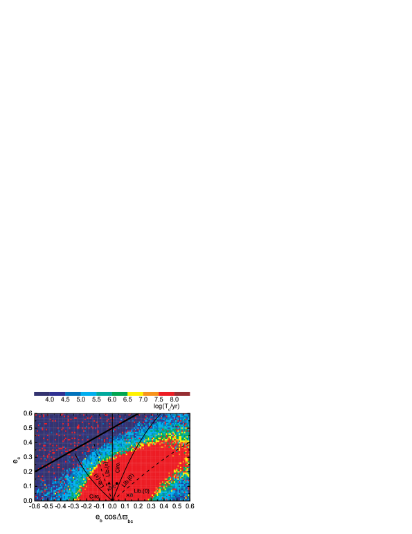
Figure 1: Various motions and orbital crossing timescale $T_{c}$ for orbits initiated from the representative plane $(e_{b}\cos\Delta\varpi_{bc},~{}e_{c})$. In the right (left) half-plane, the initial $\Delta\varpi_{bc}=0$ ($\Delta\varpi_{bc}=\pi$, respectively). The dashed curves locate the equilibriums of the secular system with $\Delta\varpi_{bc}(t)\equiv 0$ or $\Delta\varpi_{bc}(t)\equiv\pi$. The thin solid lines separate the domains that $\Delta\varpi_{bc}(t)$ librates about $0$/$\pi$ from circulation. The thick solid line in the upper-left corner shows the boundary above which $a_{b}(1+e_{b})<a_{c}(1-e_{c})$. The region in red is stable (without orbital crossing) in full three-body integration up to $10^{8}$ years. The regions in blue are unstable with $T_{c}\leq 10^{4}$ years. Between them are chaotic regions with $T_{c}\sim 10^{4-8}$ years. Motions originating from points with notation (a-c) are plotted in Fig. 2.

To investigate the secular dynamics of the two planets, we adopt the method of representative plane of initial conditions (Michtchenko & Malhotra 2004). Due to the existence of four center of mass integrals, the planar three-body (the star and two planets) system is a Hamiltonian one with four degrees of freedom, with the Hamiltonian function (e.g., Laskar & Robutel 1995):

$$H=-\sum_{i=b}^{c}\frac{\mu_{i}^{2}m^{\prime 3}_{i}}{2L_{i}^{2}}-G\frac{m_{b}m_{c}}{|{\bf r}_{b}-{\bf r}_{c}|}+\frac{m_{b}m_{c}}{m_{\ast}}(\dot{x}_{b}\dot{x}_{c}+\dot{y}_{b}\dot{y}_{c}),$$ (2)

where $\mu_{i}=G(m_{\ast}+m_{i})$, $m^{\prime}_{i}=m_{i}m_{\ast}/(m_{\ast}+m_{i})$, $L_{i}=m^{\prime}_{i}\sqrt{\mu_{i}a_{i}}$ , with $a_{i}$, $e_{i}$, ${\bf r}_{i}$ being the semi-major axis, eccentricity, relative position vector of $m_{b}$ or $m_{c}$, respectively. An averaged system is obtained by eliminating the short periodic terms,

$$H_{\rm{sec}}=-\frac{1}{(2\pi)^{2}}\int_{0}^{2\pi}\int_{0}^{2\pi}Hd\lambda_{b}\lambda_{c},$$ (3)

where $\lambda_{b},~{}\lambda_{c}$ are the longitudes of mean motion of $m_{b}$ and $m_{c}$ respectively. Due to the D’Alembert’s rule, only $\Delta\varpi_{bc}=\varpi_{c}-\varpi_{b}$ appears in the average Hamiltonian, thus the secular system is integrable with one degree of freedom in $\Delta\varpi_{bc}$ and its conjugate momentum $K_{b}=L_{b}\left(1-\sqrt{1-e_{b}^{2}}\right)$ , and $\Delta\varpi_{bc}$ either circulates or liberates around $0$ or $\pi$. So the information of secular motion with different initial conditions can be presented in the representative plane $(e_{b}\cos\Delta\varpi_{bc},~{}e_{c})$, where $\Delta\varpi_{bc}$ is fixed at either $0$ or $\pi$.

Fig.1 shows the various motions in the representative plane of the OGLE-06-109L system, with the semi-major axes of the planets being the nominal values (Table 1). Two families of the equilibriums of the secular system (3), with $\Delta\varpi_{bc}(t)\equiv 0$ or $\pi$ are plotted as dashed lines. Nearby orbits are with $\Delta\varpi_{bc}(t)$ librating around $0$ or $\pi$. Between the two libration regions are orbits with $\Delta\varpi_{bc}$-circulating, bounded by thin solid lines. We also plot the orbital crossing time ($T_{c}$) of orbits originating from the representative plane by full three-body integrations (with other angles randomly chosen). $T_{c}$ is defined as the minimum time that either $a_{b}>a_{c}$ occurs or the separation of $m_{b}$ and $m_{c}$ is smaller than one mutual Hill radii. From Fig.1, we see that apsidal alignment ($\Delta\varpi_{bc}\approx 0$) between $m_{b},~{}m_{c}$ can stabilize the interacting planets.

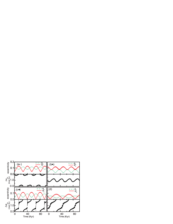
Figure 2: Some typical evolution of orbits originating from the representative plane of Fig.1. Panel (a) shows the motion with $\Delta\varpi_{bc}$ librating around 0. Panel (b) is the motion of which $\Delta\varpi_{bc}$ librates around $\pi$. Panel (c) is an example of near-separatrix motion: $e_{b}$ is periodically back to $\sim 0$ , which is similar to the orbits of the Jupiter-Saturn system in Panel (d).

Some typical motions originating from Fig.1 are plotted in Fig.2. Orbits (a), (b) are from the libration region so that $\Delta\varpi_{bc}$ librates around $0$ or $\pi$, respectively. Orbits (c) are with $\Delta\varpi_{bc}$ circulating and $e_{c}$ is in a near-separatrix motion, i.e., oscillates between 0 and a finite value ($\sim 0.1$) periodically, which is very similar to the Jupiter-Saturn system in panel (d).

2.3 Stable regions of the two-planet system

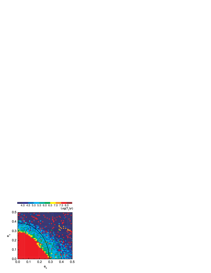
Figure 3: Orbital crossing time $T_{c}$ in $e_{b},~{}e_{c}$ plane for the two giant planets in the nominal locations (Table 1). All the other angles $\varpi_{b},~{}\varpi_{c},~{}M_{b},~{}M_{c}$ are random chosen. The solid curve plots Hill stability criterion given by Eq.(5).

We integrate the three-body system with a second-order WHM code (Wisdom & Holman 1991) from the SWIFT package (Levison & Duncan 1994). The time step is set as the $1/12$ of the period of the innermost orbit. Taking initial $a_{b}$ and $a_{c}$ with present nominal values, we carry out 2500 runs of integrations with different initial eccentricities. All the angles including $\varpi_{b}$ and $\varpi_{c}$ are random chosen. The orbital crossing time $T_{c}$, defined as the minimum time that $a_{b}>a_{c}$ or distance of $m_{b}$ and $m_{c}$ being smaller than one mutual Hill radius, is presented in Fig.3. According to the results, the two-planet ($m_{b}$ and $m_{c}$) system is stable ($T_{c}>10^{8}$yrs) only if

$$e_{b}^{2}+e_{c}^{2}<0.3^{2}$$ (4)

holds approximately. Let us compare this to another commonly used stability. Hill stability requires the ordering of the two planets remain unchanging for all the time, which allows the outer planet escaping to infinity. Topological studies of three-body systems give the following sufficient criterion for two planets being Hill stable (Marchal & Bozis 1982; Gladman 1993),

$$-\left(\frac{2m_{\rm{tot}}}{G^{2}m^{3}_{\rm{pair}}}\right)L^{2}E>1+\frac{3^{4/3}m_{b}m_{c}}{m_{\ast}^{2/3}(m_{b}+m_{c})^{4/3}}+\cdots,$$ (5)

where $m_{\rm{tot}}=m_{\ast}+m_{b}+m_{c}$, $m_{\rm{pair}}=m_{\ast}m_{b}+m_{\ast}m_{c}+m_{b}m_{c}$, $L$ and $E$ are the total angular momentum and energy of the three-body system, respectively. This criterion is also plotted in Fig.3. Note that the Hill stability criterion gives a larger region as that of $T_{c}>10^{8}$ years. This implies that, the stability defined by orbital crossing time $T_{c}>10^{8}$ years is stronger than the Hill stability, in the sense that, our stability in terms of orbital crossing requires the mutual distance of two planets being more than one mutual Hill radius all the time.

2.4 Stability of fictitious planets

We numerically integrate the orbits of a few hundred test particles in the planetary system. Such simulations enable us to identify regions where low-mass companions can have stable orbits (Rivera & Haghighipour 2007; Haghighipour 2008). The test particles are initially located in circular orbits coplanar with two planets, with their mean longitudes randomly set. The orbital evolution time is set as 100 Myrs. A particle is removed from the simulation when its stellar distance exceeds 30 AU, or it enters the Hill sphere of either planet. We study two cases that either $m_{b}$ and $m_{c}$ are in 3:1 MMR or not. In the non-resonance cases, $m_{b}$ and $m_{c}$ are initially located at the nominal elements (Table 1) with $e_{b}=0.06$ (a value inferred from formation scenario in next section). To show the dependence of stability on $\Delta\varpi_{bc}$, we let initially $\varpi_{b}=0$, $M_{b}=0$, and $\varpi_{c}=0,~{}\pi/2,~{}\pi$. $M_{c}$ is randomly set. In the 3:1 MMR cases, $m_{b},~{}m_{c}$ are set with nominal parameters except $a_{b}=2.11445$ AU, $e_{b}=0.06$, $\varpi_{b}=\varpi_{c}=M_{b}=0$, $M_{c}=\pi$, so that $m_{b}$ and $m_{c}$ are initially in 3:1 MMR, and the three corresponding resonance angles, $3\lambda_{c}-\lambda_{b}-2\varpi_{b}$, $3\lambda_{c}-\lambda_{b}-\varpi_{b}-\varpi_{c}$, $3\lambda_{c}-\lambda_{b}-2\varpi_{c}$, liberate around $\pi,~{}0,~{}\pi$, respectively.

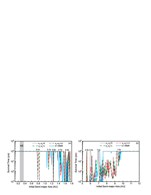
Figure 4: Lifetime of test particles in OGLE-06-109L system at different semi-major axes. Mean motion resonances are marked on the top (e.g. 5:1b means the 5:1 MMR with $m_{b}$). The grey band in (a) shows the extension of the habitable zone.

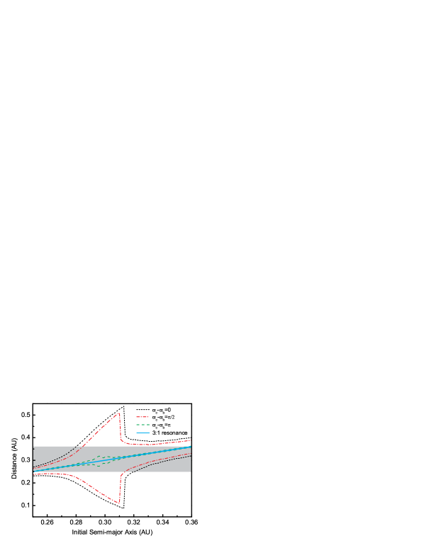
Figure 5: The largest and smallest stellar distances of an Earth-mass planet with different initial semi-major axes. $m_{b}$ and $m_{c}$ are initially put at the nominal locations and eccentricities ($e_{b}=0.06$) except the 3:1 MMR case, where $a_{b}=2.11445$ AU. The grey band is the extension of the habitable zone.

Inner region. Fig.4a shows the survival time of test particles in inner system with different initial semi-major axes. When $m_{b}$ and $m_{c}$ are not in 3:1 MMR, test particles with initial $a\leq 1.5$ AU are stable in the sense of $T_{c}>100$ Myrs, except at 5:1, 3:1, 5:2, 2:1 MMRs with $m_{b}$. The locations of these MMRs depend on $\Delta\varpi_{bc}$. However, if $m_{b}$ and $m_{c}$ are in 3:1 MMR, the stable region is reduce a bit to $a\leq 1.4$ AU.

Outer region. Fig.4b shows the survival time of test particles in the outer system. When $m_{b}$ and $m_{c}$ are not in 3:1 MMR, the test particles are stable as long as $a\geq 9.7$ AU. However, If the two planets are in 3:1 MMR , the stable region is enlarged to $a\geq 7.5$ AU except the 1:3 MMR with $m_{c}$. It is interesting to note that, the 3:1 MMR between $m_{b}$ and $m_{c}$ increases the stable region in the outer regions.

Habitable zone. Kasting et al. (1993) estimated the width of the habitable zone (HZ), where an Earth-like planet can have liquid water on its surface, around main sequence stars. For the star with mass 0.5 $M_{\odot}$, the most conservative position of HZ is 0.25 AU-0.36 AU, and the actual HZ could be much wider than this extension, e.g., the outer edge of HZ could be 0.36 AU-0.47 AU. From Fig.4a, if the two giant planets are out of 3:1 MMR, test particles with initial semi-major axes in HZ are stable, although their eccentricities will be excited by secular resonance due to $m_{b}$ and $m_{c}$ (Malhotra & Minton 2008). To see whether the planet can maintain its orbit in the HZ, we put a planet with Earth mass in different initial locations. Fig.5 shows the largest and smallest stellar distances (Q and q ) of the Earth mass planets. The shaded area is the conservative estimation of the HZ. The great variation of $Q$ and $q$ at $a=0.28~{}\rm AU-0.32~{}AU$ is due to the secular resonance of $m_{b}$ and $m_{c}$ (Malhotra & Minton 2008). Interesting to note that, the variation of $Q$ and $q$ are small when $\Delta\varpi_{bc}=\pi$, i.e., the eccentricity excited by the secular resonance of $m_{b},m_{c}$ is small (Migaszewski et al. 2009). Also, when $m_{b},~{}m_{c}$ is in 3:1 MMR, HZ is not in their secular resonance region, so the variation of $Q$ and $q$ are also small. No matter in which type of $\Delta\varpi_{bc}$, most of orbits are in HZ except $a\in[0.28~{}\rm AU,~{}0.32~{}AU]$ with $\Delta\varpi_{bc}=0,~{}\pi/2$. Considering the actual HZ is wider than this, OGLE-06-109L is a hopeful candidate system for hosting a habitable terrestrial planet. Simulations in next section indeed show the evidence for the formation of super-Earth planets in its HZ.

3 Formation Scenarios of Eccentricity

In this section, we test the previously mentioned three scenarios for the eccentricity excitation between the two giant planets in OGLE-06-109L system: (i) convergent migration and resonance trap model, where the eccentricities are excited by the trap of 3:1 MMR during the type II migrations of two planets; (ii) planetary scattering model: the eccentricities are generated by close encounters between some leftover embryos and the planets; (iii) divergent migration and MMR crossing model, when the eccentricities are excited by the crossing of either 2:1 or 3:1 MMR during the planetesimal-driven divergent migration. To simplify the problem, we assume the system has already in its later stage of formation so that both giant planets have already formed with their present masses, coexisting with tens of residue embryos with masses in the range of $0.1~{}M_{\oplus}-10~{}M_{\oplus}$ (Earth mass).

For a planet embedded in a geometrically thin and locally isothermal disk, angular momentum exchanges between the planet and the gas disk will cause a net momentum lose on the planet, which results in a fast and so called type I migration of the planet Goldreich & Tremaine (1979); Ward (1997); Tanaka et al. (2002). Some mechanisms are proposed recently to reduce the speed or even reverse the direction of migration. Laughlin et al. (2004), Nelson & Papaloizou (2004) proposed that, in the locations where the magnetorotation instability (MRI) is active, gravitational torques arising from megnetohydrodynamical turbulence will contribute a random walk component to the migratory evolution of the planets, thus prolong the drift timescale. Paardekooper & Mellema (2006) noticed that the inclusion of radiative transfer can cause a strong reduction in the migration speed. Subsequently investigations (Baruteau & Masset 2008; Kley & Crida 2008; Paardekooper & Papaloizou 2008) indicated that the migration process can be slowed down or even reversed for sufficiently low mass planets. Through full 3D hydrodynamical simulations of embedded planets in viscous, radiative discs, Kley et al. (2009) confirmed that the migration can be directed outwards up to planet masses of about 33 $M_{\oplus}$. Due to the vagueness of type I migration, we do not consider this effect at the present paper. A detailed study of formation of Earth-like planets in OGLE-06-109L system, which includes the type I migration of embryos, will be presented in a subsequent paper (Wang & Zhou, in preparation).

3.1 Disk model

According to the conventional core accretion scenario of planet formation, planet formed through planetesimals coagulation by means of runaway growth and became protoplanetary embryos by oligarchic growth in the protoplanetary disk (Safronov 1969; Kokubo & Ida 1998). To model the masses of embryos formed in disk, we adopt the empirical minimum mass solar nebula (hereafter MMSN, Hayashi 1981) so that the surface density of gas disk at stellar distance $a$ is given as

$$\Sigma_{g}=2.4\times 10^{3}f_{g}f_{\rm dep}(\frac{a}{\rm 1AU})^{-3/2}~{}{\rm g~{}cm}^{-2},$$ (6)

where $f_{g}$ is the gas enhancement factor, $f_{\rm dep}=\exp(-t/\tau_{\rm dep})$ is the gas depletion factor due to disk accretion, photoevaporation or planet formation with a timescale of $\tau_{\rm dep}\sim 3$ Myrs (Haisch et al 2001), $t$ is the evolution time. The surface density of solid disk is given as,

$$\Sigma_{d}=10f_{d}\gamma_{\rm ice}(\frac{a}{\rm 1AU})^{-3/2}~{}{\rm g~{}cm}^{-2},$$ (7)

where $f_{d}$ is the solid enhancement factor, $\gamma_{\rm ice}$ is the volatile enhancement with a value of 4.2 or 1 for material exterior or interior to the snow line (0.68 AU for OGLE-06-109L system), respectively. In such a disk, the embryos will grow under cohesive collisions in a timescale of (Kokubo & Ida 2002; Ida & Lin 2004)

$$\tau_{acc}\simeq 1.6\times 10^{5}\gamma_{\rm ice}^{-1}f_{d}^{-1}f_{g}^{-2/5}(\frac{a}{\rm 1AU})^{27/10}$$

$$\times(\frac{M_{c}}{M_{\oplus}})^{1/3}(\frac{M_{*}}{M_{\odot}})^{-1/6}~{}{\rm yr},$$ (8)

where $M_{c}$ is the core mass. The core growth will continue until it accretes all the dust material round its feeding zone ($\sim 10$ Hill radii) so that an isolation body is achieved with mass of (Ida & Lin 2004)

$$M_{\rm iso}=0.12\gamma_{\rm ice}^{3/2}f_{d}^{3/2}(\frac{a}{\rm 1AU})^{3/4}(\frac{M_{*}}{M_{\odot}})^{-1/2}M_{\oplus}.$$ (9)

For the OGLE-06-109L system, the isolation mass at 4 AU with $f_{d}=2$ is around $12~{}M_{\oplus}$, above the critical mass $(\sim 10~{}M_{\oplus}$) for the onset of efficient gas accretion to form giant planets (Pollack et al. 1996), and the core growth timescale is $\sim 1.2$ Myrs.

Interactions between embryos and the gas disk may damp the eccentricities of the embryos (Goldreich & Tremaine 1980). The timescale of the eccentricity-damping for an embryo with mass $m$ can be described as (Cresswell & Nelson 2006),

$$(\frac{e}{\dot{e}})_{\rm emb}=\frac{Q_{e}}{0.78}(\frac{M_{*}}{m})(\frac{M_{*}}{a^{2}\Sigma_{g}})(\frac{h}{r})^{4}\Omega^{-1}[1+\frac{1}{4}(e\frac{r}{h})^{3}]~{}{\rm yr},$$ (10)

where $r$, $e$, $h$, $\Omega$ are the stellar distance, eccentricity of the embryo, scale height of the disk and the Kepler angular velocity, respectively, $Q_{e}=0.1$ is a normalization factor to fit with hydrodynamical simulations.

As an embryo grows to a massive planet ($\geq 30~{}M_{\oplus}$), it will induce strong tidal torques on the disk to open a gap around it (Lin & Papaloizou 1993). Then the planet will be embedded in the viscous disk to undergo type II migration. The timescale of type II migration for a planet with mass $m_{p}$ can be modelled as (Ida & Lin 2004)

$$\tau_{\rm II}=\frac{a}{|\dot{a}|}=0.8\times 10^{6}~{}{\rm yr}~{}f_{g}^{-1}(\frac{m_{p}}{M_{\rm Jup}})(\frac{M_{*}}{M_{\odot}})^{-1/2}$$

$$\times(\frac{\alpha}{10^{-4}})^{-1}(\frac{a}{\rm 1AU})^{1/2},$$ (11)

where $\alpha$ is a dimensionless parameter to adjust the effective viscosity, and we set $\alpha=10^{-4}$ as a standard value in our simulation. When a giant planet is embedded in a gas disk, tidal interaction of disk may damp its eccentricity if it is not massive enough. As we mentioned in the abstract, the situation is quite elusive for different mass regime of the giant planets, so we adopt an empirical formula (Lee & Peale 2002)

$$(\frac{\dot{e}}{e})_{\rm pl}=-{\rm K}\left|\frac{\dot{a}}{a}\right|$$ (12)

to describe the eccentricity-damping rate of giant planets in the OGLE-06-109L system, where K is a positive constant with a value ranging $10-100$ Sándor et al. (2007). After some tests, we choose $K=10$ in this paper to let $e_{b}$ and $e_{c}$ have reasonable convergent values.

3.2 Numerical simulations

In this section, we simulate the configuration formation for the OGLE-06-109L system with N-body models. We assume the two giant planets have formed with the observed masses at 4 AU and 8 AU-9 AU respectively. The physical epoch corresponds to this assumption is $\sim 1$ Myrs after the formation of star, so that the gas disk is still present. The two giant planets have opened gaps around them and will undergo type II migration according to equation (11) in the viscous disk. At the initial stage of our simulation, there are some leftover embryos in inner orbits that have obtained their isolation masses. To mimic the formation of Earth-like planets in inner orbits, we put 18 embryos, with masses ranging from $0.17~{}M_{\oplus}$ to $9~{}M_{\oplus}$ derived from equation (9) and initial locations from 0.25 AU to 3 AU. The mutual distances among the embryos are set as 10 Hill radii. An additional embryo with in situ isolation mass will be put between $m_{b}$ and $m_{c}$ in model 2. All the planets and embryos are initially located in near-coplanar and near-circular orbits ($e=10^{-3}$, inclination $i=e/2$), their phase angles (mean motion, longitude of perihelion, longitude of ascending node) are randomly chosen. The acceleration of the planet (embryo) with mass $m_{i}$ is given as,

$$\frac{d}{dt}\textbf{V}_{i}=-\frac{G(M_{*}+m_{i})}{{r_{i}}^{2}}(\frac{\textbf{r}_{i}}{r_{i}})~{}~{}~{}~{}~{}~{}~{}~{}$$

$$+\sum_{j\neq i}^{N}Gm_{j}[\frac{(\textbf{r}_{j}-\textbf{r}_{i})}{|\textbf{r}_{j}-\textbf{r}_{i}|^{3}}-\frac{\textbf{r}_{j}}{r_{j}^{3}}]$$

$$+\textbf{F}_{\rm edamp}(+\textbf{F}_{\rm migII}),~{}~{}~{}~{}~{}~{}~{}~{}~{}$$ (13)

where $\textbf{r}_{i},\textbf{V}_{i}$ are the position and velocity vectors of $m_{i}$ in the stellar-centric coordinates,

$$\textbf{F}_{\rm edamp}=-2\frac{(\textbf{v}_{i}\cdot\textbf{r}_{i})\textbf{r}_{i}}{r_{i}^{2}\tau_{e}}$$ (14)

is damping acceleration, effective for all embryos and gas giants but with different $\tau_{e}$ in equations (10) and (12), respectively, and the acceleration that causes the type II migration,

$$\textbf{F}_{\rm migII}=-\frac{{\bf V}_{i}}{2\tau_{\rm II}}$$ (15)

is adopted for two giant planets. We numerically integrate the evolution of equation (13) with a time-symmetric Hermit scheme (Aarseth 2003). The simulation is performed up to 10 Myrs. As we assume that the gas disk depletes exponentially in a timescale $\tau_{\rm dep}=1$ Myrs, the gas disk almost disappears at the end of simulation.

During the earlier stage when gas disk is present (the coming models 1-2), embryos in outer disk will also induce a damping of giant planets’ eccentricities through dynamic friction, which has similar effect by gas disk. However, as the gas disk dominates before gas depletion, we did not consider the presence of embryos in outer disk in models 1-2, except in model 3 where embryos in outer disk are included, after the gas disk depletes.

Table 2: Initial parameters for two giant planets (i-pl) and embryos (i-emb) in numerical simulations of model 1 and 2 in section 3.2, with the outcomes of the survival embryos (f-emb) and giant planets (f-pl). $P_{c}/P_{b}$ is the period ratios of two giants at 10 Myrs, the end of our simulations.

ID	i-pl’s	i-emb.’s	i-emb.’s	i-emb.’s	f-emb’s	f-pl’s a (AU)
	a (AU)	No.	masses ($M_{\oplus}$)	a (AU)	No.	and ($P_{c}/P_{b}$)
R1	3.8, 8.5	18	[0.17, 8.94]	[0.25, 2.8]	4	2.53, 5.26; 3:1
R2	4, 8	19	[0.17, 9.42], 16.8	[0.26, 3], 6.5	1	2.40, 5.63; 3.60
R3	4, 8.2	19	[0.17, 9.42], 16.8	[0.26, 3], 6.5	11	2.83, 5.02; 2.35

Model 1: smooth and convergent migration. In this model, we vary the initial locations of two giant planets, $a_{b}$ and $a_{c}$. The 18 embryos with in situ isolation masses in inner orbits are put so that the outermost one is in an orbit $3.5$ Hill Radii away from $m_{b}$. During the evolution of the typical run R1 ( See Table 2 for initial parameters), $m_{b}$ and $m_{c}$ are captured into 3:1 MMR at $t\approx 1$ Myrs, with three resonant angles liberate around either $0$ or $\pi$ with amplitudes around $\sim 0.4~{}\pi$ (Fig.6). Their eccentricities are excited to about 0.1 inside the resonance. Eccentricities of the embryos in the inner orbits are also excited due to secular perturbations from two giant planets, which results in their inward migration in the gas disk. At the end of simulation, they merge into 4 planets at [0.22 AU,  0.77 AU], with masses of 4.86 $M_{\oplus}$, 8.76 $M_{\oplus}$, 5.79 $M_{\oplus}$, 16.06 $M_{\oplus}$ in the order of increasing semi-major axes. Noticeably, the inner two are in the edge of the habitable zone ([0.25 AU,  0.36 AU]) of the system.

The mechanism that migration of giant planets triggers the merge of inner embryos in MMRs or secular resonances had been already discussed in many literatures, e.g., Zhou et al. (2005), Fogg & Nelson (2005). However, in this case, the eccentricities of embryos are excited by the secular perturbations of outside giant planets. The configuration of 3:1 MMR between two planets are kept to the end of the simulation, when they are stalled at 2.53 AU and 5.26 AU due to the severe depletion of gas disk. We did 8 runs in this model with $a_{b}$ varying in [3.5 AU,  3.8 AU], and $a_{c}$ in [8.2 AU,  8.5 AU]. In all the simulations, the two giant planets are trapped in 3:1 MMR, with their eccentricities osculating around $\sim 0.1$ at the end of evolution as in Fig.6c.

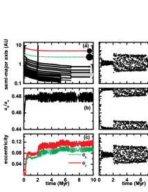
Figure 6: Evolution of orbits in model 1 (R1 in Table 2). The two giants ($m_{b},~{}m_{c}$) are put initially at near-circular orbits with $a_{b}=3.8$ AU and $a_{c}=8.5$ AU. 18 embryos with in situ isolation masses are put in inner orbits. Panel (a): Evolution of semi-major axes of the 2 planets and 18 embryos. The grey band shows the extension of the habitable zone. The green dash lines represent the evolution of planet b and the red solid lines show the result of planet c as the same meaning in panel (c). Panel (b): Evolution of semi-major axis ratio of two giant plants. Panel (c): Eccentricity evolution of the two giant planets. Panel (d, e, f): Evolutions of the resonance angles for the 3:1 MMR between $m_{b}$ and $m_{c}$. $\theta_{1}=3\lambda_{c}-\lambda_{b}-2\varpi_{b}$, $\theta_{2}=3\lambda_{c}-\lambda_{b}-\varpi_{b}-\varpi_{c}$, $\theta_{3}=3\lambda_{c}-\lambda_{b}-2\varpi_{c}$.

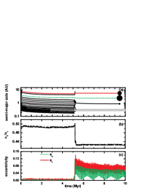
Figure 7: Evolution of orbits in model 2 (R2 in Table 2). The two giant planets ($m_{b},~{}m_{c}$) are put initially at near-circular orbits with $a_{b}=4$ AU and $a_{c}=8$ AU. The 18 embryos in inner orbits are put initially as in Fig.6. An additional embryo is put at 3.5 Hill radii inside the orbit of $m_{c}$. Panel (a): Evolution of semi-major axes of the 2 planets and 19 embryos. The grey band shows the extension of the habitable zone. The green dash lines represent the evolution of planet b and the red solid lines show the result of planet c as the same meaning in panel (c). Panel (b): Evolution of semi-major axis ratio of two giant plants. Panel (c): Eccentricity evolution of the two giant planets.

Model 2: Planetary scattering during migration. Unlike the previous model that $m_{b}$ and $m_{c}$ undergo smooth migration, now, besides the 18 embryos in inner orbits, we put an additional embryo with local isolation mass (denoted as $m_{\rm e1}$, slightly varies for different locations) between the orbits of $m_{b}$ and $m_{c}$. Fig.7 shows the results of a typical run (R2), with $m_{\rm e1}=16.8~{}M_{\oplus}$. At $t\approx 5.2$ Myrs, a close encounter between $m_{c}$ and $m_{\rm e1}$ occurred, which scatters $m_{e1}$ out of the system (Fig.7). The encounter excites $e_{c}$ up to $0.1$, which in turn excites $e_{b}$ from 0 to $\sim 0.08$, resulting in a configuration that $e_{b}$ passing $0$ in the eccentricity plane ($e_{b}e_{c}\cos\Delta\varpi_{bc}$, $e_{b}e_{c}\sin\Delta\varpi_{bc}$) almost periodically, the so called near-separatrix (of libration and circulation of $\Delta\varpi_{bc}$) motion (Barnes & Greenberg 2006, 2008). The eccentricities of embryos in inner orbits are also excited due to the sudden increase of $e_{b}$ and $e_{c}$, which cause strong mergers among the embryos into a planet of 14.38 $M_{\oplus}$ at 0.89 AU.

If close encounters between $m_{e1}$ and one of the giant planets occur much earlier, tidal interaction between the planets (embryos) and the gas disk will eventually damp their eccentricities. In run R3, the scattering process occurred at $t=1.5$ Myrs when the eccentricity-damping induced by the gas disk is still strong (Fig.8). As a result, $e_{b}$ and $e_{c}$ that excited during planetary scattering are damped to less than 0.01 quickly. In this case, 11 planets are left with their masses from 0.21 $M_{\oplus}$ to 16.81 $M_{\oplus}$ at [0.15 AU,  1.10 AU]. Among them, 2 embryos are in the habitable zone.

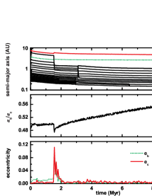
Figure 8: Evolution of orbits in model 2 (R3 in Table 2). The two giants ($m_{b},m_{c}$) are put initially at near-circular orbits with $a_{b}=4$ AU and $a_{c}=8.2$ AU. The 18 embryos in inner orbits are put initially as in Fig.6. An additional embryo is put at 3.7 Hill radii inside the orbit of $m_{c}$. Panel (a): Evolution of semi-major axes of the 2 planets and 19 embryos. The grey band shows the extension of the habitable zone. The green dash lines represent the evolution of planet b and the red solid lines show the result of planet c as the same meaning in panel (c). Panel (b): Evolution of semi-major axis ratio of two giant plants. Panel (c): Eccentricity evolution of the two giant planets.

We did 20 runs of simulations with different initial locations of $m_{e1}$. Among them, 6 runs have close encounter events during the evolution, like run R2, resulting in similar configurations of $m_{b}$ and $m_{c}$ as in Fig.7. 5 runs have earlier close encounters so that $e_{b}$ and $e_{c}$ are damped in the end of simulations. The rest 9 runs do not suffer close encounters, but have some milder encounter events occasionally. The resulting $e_{b}$ and $e_{c}$ have only slight changes up to $\sim 0.01$.

In a compact configuration with $a_{b}/a_{c}>0.48$, semi-major axes shift to $a_{b}/a_{c}<0.48$ by planetary scattering is a possible routine that could lead to the trap of 3:1 MMR between $m_{b}$ and $m_{c}$. To investigate this probability, we perform additional 900 runs of simulations with a simplified four-body (star-two giants-one embryo) model. In this model, $m_{b}$ and $m_{c}$ are located initially at 3.7 AU and 7.6 AU so that $(a_{b}/a_{c}>0.48)$ , with one embryo $m_{e1}$ between their orbits. The initial semi-major axis of $m_{e1}$ is chosen at [5.0 AU,  5.4 AU]. The mass of $m_{e1}$ slightly varies at different locations, in the range of $13.8~{}M_{\oplus}-14.6~{}M_{\oplus}$. Both $F_{\rm edamp}$ and $F_{\rm migII}$ in Eqs. (14) and (15) are included. Numerical simulations show that, 185 runs out of 900 ones with close encounter events occurred between $m_{e1}$ and one of the planets. The epoch for close encounters occurred do not show a clear correlation with the relative distance between the embryo and one of the giant planets (Fig.9). Among the 185 runs with scattering events, 21 runs ($2.3\%$ of 900 runs) lead to the trap of $m_{b}$ and $m_{c}$ into 3:1 MMR, 11 runs ($1.2\%$) result in the trap near the boundary of 3:1 MMR, the rest 153 runs ($17.0\%$) do not lead to the trap of 3:1 MMR. We also observe 62 runs with $m_{b}$ and $m_{c}$ being trapped in 8:3 MMR. Fig.10 shows the final $e_{b},~{}e_{c}$ at the end of 900 runs’ simulations. As we can see, besides those being trapped into 8:3 MMR, $e_{b}$ and $e_{c}$ are excited significantly only in those 185 runs with planetary scattering, with the average values $e_{b}\sim 0.058$ and $e_{c}\sim 0.085$ (Fig.10).

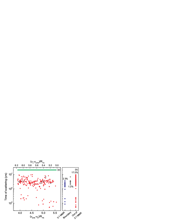
Figure 9: Orbital crossing time of the 900 simulations with four-body model (star-two planets-embryo). Panel (a): Orbital crossing time versus the initial position of the embryo. Separation between the embryo and the planet b measured by the planet’s Hill radius is marked below the figure, while that with the planet c is marked above the figure. Orbits without close encounter are represented by green stars; other symbols show the runs in which close encounters happen, among them blue squares indicate the runs in which the two planets are trapped into the 3:1 MMR, black circles indicate the cases in which the two planets are in the boundary of the 3:1 MMR, red circles plot the cases that the two planets are out of the 3:1 MMR. Panel (b): the proportions of each kinds of motions in the total 900 runs of simulations.

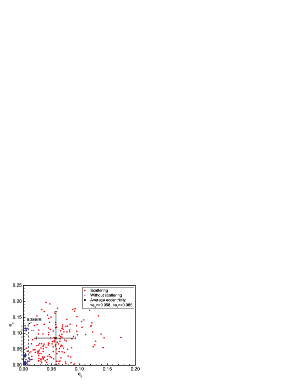
Figure 10: Final eccentricities of the two giant planets in the end of 900 runs of simulations. If no close encounter happens (indicated by blue stars), the eccentricities of the two planets are small ($\sim$ 0.005) except 62 runs in which the two planets are trapped into 8:3 MMR. In the 185 runs that close encounters happen (represented by red circles), eccentricities are excited to relatively high values. The averaged $e_{b}$ and $e_{c}$ over the 185 runs with planetary scattering are also plotted, with the error bars standing for the standard deviations.

Model 3: Divergent migration in the presence of planetesimal-disk. To study the effect of planetesimal-disk in outside orbits after the gas disk is depleted, we perform simulations by including the embryos in outside orbits but discarding those in inner orbits, since they may be in hot orbits and have less affections on the outer system. We set two types of embryos in the outer region, those with masses of $5~{}M_{\oplus}$ and of $0.2~{}M_{\oplus}$. After some test simulations, we find that the solid disk out of 10 AU has little effect on the evolutions of the two giant planets at nominal location (See Fig.11 for a typical run). So we set the outer edge of solid disk within 10 AU in following simulations. Two groups of simulations are made according to different initial $a_{b}$ and $a_{c}$.

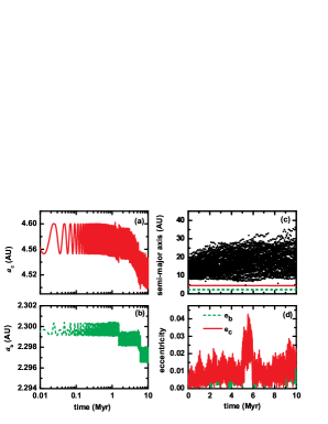
Figure 11: Evolution of a typical run in model 3 with a total disk mass of 27 $M_{\oplus}$ planetesimal disk outside in [11 AU, 16 AU]. Panel (a) and (b): evolutions of semi-major axes of two giant planets. Panel (c): semi-major axis evolutions of all planets and embryos. Panel (d): eccentricity evolutions of two giant planets.

Group 3a: We put initially $m_{b}$ and $m_{c}$ at $a_{b}=3$ AU and $a_{c}=4$ AU, so $m_{c}$ is inside the 2:1 MMR location (at $4.76$ AU) of $m_{b}$. The separation is about $3.3$ times of their mutual Hill’s radii ($R_{Hbc}$), above the threshold ($2.4~{}R_{Hbc}$), so they are Hill stable (Gladman 1993) if there is no other perturbations. We put 63 embryos evenly at [5.5AU,  9.5AU], including $5\times 5~{}M_{\oplus}$ and $58\times 0.2~{}M_{\oplus}$ ones, corresponding to a solid disk of $f_{d}=2$ with total mass of $36.6~{}M_{\oplus}$ in [5 AU,  10 AU].

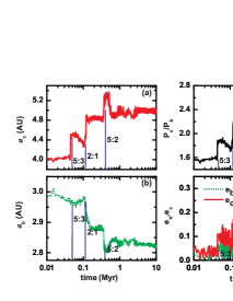
Figure 12: Evolution of two giant planets in one run of group 3a (model iii). The blue solid lines show the epoch of 5:3 MMR, 2:1 MMR and 5:2 MMR orbital crossing between the two giant planets $m_{b}$ and $m_{c}$. Panels (a), (b), (c), (d) show the evolution of semi-major axes of $m_{b}$ and $m_{c}$, period ratio ($P_{c}/P_{b}$), and eccentricities $e_{b},e_{c}$, respectively. The green dash lines represent the evolution of planet b and the red solid lines show the result of planet c in panel (a), (b) and (d).

Fig.12 shows the evolution of $m_{b}$ and $m_{c}$ in a typical run, with the innermost embryos $a_{\rm in}=5.5$ AU. Under the perturbation of outer embryos, $m_{b}$ ($m_{c}$) becomes unstable and undergoes inward (outward, resp.) migration quite soon (Fig.12a, b). The migration results in the quick crossing of $5:3$ and $2:1$ MMR at $t\approx 0.05$ Myrs, and 0.12 Myrs (see Fig.12c), the two most strong resonances between 3:2 and 3:1 MMRs, and the system seems to be stable until $m_{b}$ ($m_{c}$) reaches around 2.82 AU (4.90 AU, resp.), with a drift extension of $6\%$ ($22\%$, resp.). Their eccentricities are excited after the crossing of $5:3$ and $2:1$ MMR, with maximum values of $\sim 0.2-0.3$ (Fig.12d). Finally $e_{b}$ and $e_{c}$ oscillate in [0.03, 0.15] and [0.04, 0.19], respectively. The $5:3$ and $2:1$ MMR crossings of $m_{b}$ and $m_{c}$ lead to the strong scattering of embryos in outer orbits (Fig.13a), which results in the escape of all the embryos except one with mass $5~{}M_{\oplus}$ at the orbit of $15$ AU and eccentricity of 0.45.

We did 15 runs of simulations in this group, by changing the initial locations of the 63 embryos so that $a_{\rm in}$ of the innermost one varies in [5.2 AU,  8 AU]. $5:3$ and $2:1$ MMR crossings occurred in 3 runs, with eccentricities $e_{b}\in[0.03,~{}0.24]$ and $e_{c}\in[0.04,~{}0.28]$ at the end of our simulations ($t$=10 Myrs). We did not observe resonance-crossings in another 3 runs up to 10 Myrs’ evolution, with final eccentricities $e_{b}\in[0,~{}0.05]$ and $e_{c}\in[0,~{}0.06]$. In the rest 9 runs, $m_{b}$ and $m_{c}$ have strong close encounter so that $m_{c}$ is scattered out of the system, with the eccentricity of the only survival giant planet $m_{b}\sim 0.3$. The values of $a_{\rm in}$ corresponding to these three types of outcomes (MMR crossing, non MMR crossing, $m_{c}$ being ejected ) do not show clear correlation, which indicates the chaotic states of $m_{b}$ and $m_{c}$ under the perturbation of outer embryos.

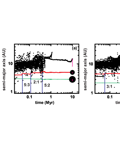
Figure 13: Evolution of two giant planets and embryos in model 3. The error bar at the end of the evolution show the extension of $a(1-e)$ of each survival planets and embryos. The green dash lines represent the evolution of planet b and the red solid lines show the result of planet c. Panel (a): semi-major axis evolutions of one run of group 3a, the blue solid lines indicate the epoch of 5:3 MMR, 2:1 MMR and 5:2 MMR orbital crossing between the two giant planets. Panel (b): semi-major axis evolutions of one run of group 3b, the blue solid lines indicate the epoch of 3:1 MMR orbital crossing between the two giant planets.

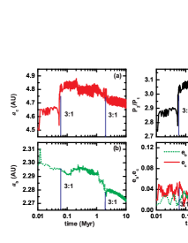
Figure 14: Evolution of two giant planets in one run of group 3b. The blue solid lines show the epoch of 3:1 MMR orbital crossing between the two giant planets $m_{b}$ and $m_{c}$. Panels (a), (b), (c), (d) show the evolution of semimajor axes of $m_{b}$ and $m_{c}$, period ratio ($P_{c}/P_{b}$), and eccentricities $e_{b},~{}e_{c}$, respectively. The green dash lines represent the evolution of planet b and the red solid lines show the result of planet c in panel (a), (b) and (d).

Group 3b: $m_{b}$, $m_{c}$ are put initially at $a_{b}=2.3$ AU and $a_{c}=4.6$ AU, the nominal locations. We put 56 embryos evenly at [6.4 AU,  10.4 AU], including $5\times 5~{}M_{\oplus}$ and $51\times 0.2~{}M_{\oplus}$ ones, corresponding to a solid disk of $f_{d}=2$ with total mass of $35.2~{}M_{\oplus}$ in [5.5 AU,  10.5 AU]. Fig.14 shows the evolution of $m_{b}$ and $m_{c}$ in a typical run, with the innermost embryos $a_{\rm in}=6.4$ AU. $m_{b}$, $m_{c}$ cross $3:1$ MMR during the divergent migration at $t\approx 0.06$ Myrs and $t\approx 2$ Myrs, causing the increase of $e_{b}$ and $e_{c}$, At the end of simulation, $m_{b}$ and $m_{c}$ locate at $2.27$ AU and $4.71$ AU, with $e_{b}\in[0.01-0.07]$ and $e_{c}\in[0.03-0.1]$. One $5~{}M_{\oplus}$ embryo (at 11.4 AU with $e=0.024$) and $4\times 0.2~{}M_{\oplus}$ ones (at [16 AU, 22 AU] and e $\in[0.08,~{}0.53]$) are left (Fig.13b).

We did totally 41 runs (13 runs with $f_{d}=2$ and 28 runs with lower $f_{d}$) in this group. For the 13 runs of $f_{d}=2$, 5 out of these 8 runs with $a_{\rm in}<7.8$ AU are observed having $m_{b},~{}m_{c}$’s 3:1 MMR crossing, with final eccentricities $e_{b}\in[0,~{}0.08]$, $e_{c}\in[0,~{}0.1]$. The rest 5 runs with $a_{\rm in}>7.8$ AU do not have 3:1 MMR crossing, with final eccentricities $e_{b}\in[0,~{}0.04]$, $e_{c}\in[0,~{}0.04]$. For the 28 runs with lower solid disks ($f_{d}=1,~{}1.2,~{}1.5,~{}1.6,~{}1.8$) and different $a_{\rm in}$, no 3:1 MMR crossing is observed in runs with $f_{d}<1.6$, maybe due to the small mass of solid disk ($M<22~{}M_{\oplus}$). While for $f_{d}=1.6,~{}1.8$, the probability of 3:1 MMR crossing is $\sim 33\%$. The extension of $e_{b}$ and $e_{c}$ are similar to that of $f_{d}=2$.

4 Conclusions and Discussions

In the paper we investigate the dynamics and formation scenario for OGLE-06-109L system in terms of the observed planets $(m_{b},~{}m_{c})$, aiming to understand its formation history and to predict $e_{b}$ that is not revealed by observation. According to the investigation, we find the evolution history of $m_{b}$ and $m_{c}$ depends strongly on the initial conditions, i.e., the cores of $m_{b}$ and $m_{c}$ before efficient gas-accretion begins.

According to the conventional core-accretion scenario of planet formation, a giant planet forms from a massive embryo ($>10~{}M_{\oplus}$) through accreting nearby gas. Embryos beyond the snow line tend to have larger isolated masses, thus they are the ideal candidates for planetary cores. However, there will be more than one embryo beyond the snow line. For example, assuming a solid disk of 2 times of the minimum mass solar nebula (MMSN) for the OGLE-06-109L system, the space between 3 AU and 8 AU can be occupied by 4-5 embryos with isolation masses above $10~{}M_{\oplus}$ and mutual separations $\sim 10$ Hill radii. Due to the long quasi-hydrostatic sedimentation stage of gas ($\sim$ several Myrs, Pollack et al. 1996), and the perturbation from first generation giant planets to nearby embryos, all isolation masses may have the chance to grow up into second generation giant planets, thus the initial locations of formed planets can not be well determined.

For the two giant planets in OGLE-06-109L system, if they formed from embryos with relatively far mutual distances, their initial configuration is loose, e.g., $a_{b}/a_{c}<0.48$, so that they are beyond the 3:1 MMR. Subsequent smooth migration under disk tide will result in a 3:1 MMR, provided suitable gas depletion timescale. We did 8 runs in model 1, all the simulations result in the two giant planets trapped in 3:1 MMR, with their eccentricities being excited and osculating around $\sim 0.1$ at the end of evolutions as in Fig.6c.

If the two planets formed from embryos with a relatively small distance, they may have a compact configuration initially with $a_{b}/a_{c}>0.48$. Then planetary scattering among residue embryos $(m_{e1})$ and planets are most probably the major cause of $e_{b}$ and $e_{c}$. Among the 900 simulations of model 2 we did, 185 runs ($20.5\%$) with close encounter events occurred between $m_{e1}$ and one of the planets, with the average values $e_{b}\sim 0.058$ and $e_{c}\sim 0.085$ (Fig.10). Only $3.5\%$ of the 900 runs lead to the trap (or in the boundary) of $m_{b}$ and $m_{c}$ into 3:1 MMR.

After the gas disk is almost depleted, divergent migration of $m_{b}$ and $m_{c}$ caused by the residue embryos and planetesimals in outer disk may drive $m_{b}$ and $m_{c}$ passing through lower order MMRs. According to our simulations of model 3, the crossing of 2:1 MMR is unlikely in the OGLE-06-109L system, as it will excite eccentricities of $m_{b}$ and $m_{c}$ up to $0.2-0.3$, and it is easy to eject $m_{c}$ out of the system. On the other hand, the crossing of 3:1 MMR is likely, which will excite the eccentricities up to $e_{b}\sim 0.06$ and $e_{c}\sim 0.10$. However, from our simulations, the required migration depends on the mass and radial location of the planetesimal disk. A solid disk with mass enhancement factor $f_{d}\geq 2$ over the minimum solar nebular may be needed, with their inner edge within $7.8$AU. Considering the similarities of solar system and the OGLE-06-109L system, $f_{d}\sim 2$ is still possible for the OGLE-06-109L system with a stellar mass $\sim 0.5~{}M_{\odot}$.

In summary, all the three models (i) smooth, convergent migration and the trap of 3:1 MMR; (ii) planetary scattering; (iii) divergent migration and the crossing of 3:1 MMR, $e_{b}$ and $e_{c}$ can be excited. However, the probabilities, the conditions and the final outcomes of these three models are different. Smooth and convergent migration in model (i), if it occurs as predicted by the standard model, could result steadily in the trap of 3:1 MMR between $m_{b}$ and $m_{c}$, with $e_{b},~{}e_{c}\sim 0.1$ all the time. For model (ii), the probability of planetary scattering occurs is $\sim 20\%$, they result in average $e_{b}\sim 0.06$ and $e_{c}\sim 0.09$, and $m_{b}$ is more likely to undergo a near-separatrix motion in ($e_{b}e_{c}\cos\Delta\varpi_{bc},~{}e_{b}e_{c}\sin\varpi_{bc}$), i.e., $e_{b}$ passing 0 at a secular timescale ($\sim 0.08$ Myrs as in Fig.15a). The probability for $m_{b},~{}m_{c}$ 3:1 MMR crossing in model (iii) depends on the mass and extension of residue solid disk, and will result in $e_{b}\in[0.01-0.07]$ and $e_{c}\in[0.03-0.1]$, but the variations in these ranges are in a relative shorter timescale, e.g., $\sim$ 0.01 Myrs in Fig.15b.

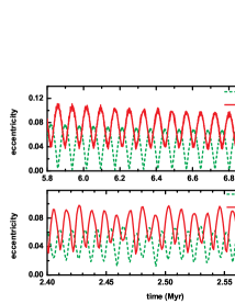
Figure 15: Eccentricity evolutions of a typical run in model (ii) and model (iii). Panel (a): zoomed in evolution of figure 7c from 6 Myrs to 7 Myrs, with $a_{b}\approx 2.40$ AU and $a_{c}\approx 5.65$ AU. Panel (b): zoomed in evolution of figure 14d from 2.4 Myrs to 2.6 Myrs, with $a_{b}\approx 2.28$ AU and $a_{c}\approx 4.73$ AU.

Some analytical estimations of related timescale is helpful to reveal the different procedures corresponding to eccentricity evolution in model (ii) and (iii). The timescale for the secular evolution of two planets is given as $2\pi/|g_{1}-g_{2}|$, where $g_{1},~{}g_{2}$ are the two eigenfrequencies (Murray & Dermott 1999, Zhou & Sun 2003). This gives 0.076 Myrs and 0.037 Myrs for orbits in Fig.15a and Fig.15b, respectively. In the circular restricted three-body (CRTB) framework, the timescale of a massless body in the 3:1 MMR of a perturber is estimated as $2\pi/(ne\sqrt{3\mu^{\prime}\alpha f_{d}(\alpha)})$, where $\mu^{\prime}=m^{\prime}/m_{*}$ is the mass ratio of the perturber, $n,e$ is the mean motion and eccentricity of the massless body, $f_{d}(\alpha)$ is the function of Laplace coefficients of semi-major axis ratio $\alpha$ (Murray & Dermott 1999). Assuming $m_{b}$ is the perturber, $e=0.04$ gives the $e$-evolution timescale of $m_{c}$ in $m_{b}$’s 3:1 MMR as 0.01 Myrs, although the CRTB model is not a good model here. So the eccentricity evolution of Fig.15a is due to the secular dynamics, while that in Fig.15b is due to the 3:1 MMR crossing. We also find such a 3:1 MMR timescale is kept for these two orbits up to the end of simulation.

So to understand scenarios of eccentricity formation for the OGLE-06-109L system, we need more detailed information of their orbits. If $m_{b}$ and $m_{c}$ are shown by observation that they are in 3:1 MMR, then model (i) should be the most possible scenario. Based on our simulations in section 2.1, we think the possibility that $m_{b},~{}m_{c}$ in 3:1 MMR is small, thus model (i) is unlikely. However, either model (ii) or (iii) can not be decided by the present observations. In both models, the averaged $e_{c}\sim 0.09-0.10$, roughly agrees with the observed value $0.11_{-0.04}^{+0.17}$, and predict the most possible value of $e_{b}\approx 0.06$. If $m_{b}$ and $m_{c}$ are observed to undergo a near separatrix motion in ($e_{b}e_{c}\cos\Delta\varpi_{bc},~{}e_{b}e_{c}\sin\varpi_{bc}$) plane in a timescale of secular motion, then model (ii) is favored for the origin of eccentricities. And we can infer that, after OGLE-06-109L b and c formed, either smooth migration history during the presence of gas disk is short, or during their migration history, embryos may suffer close encounter with the planets, exciting their eccentricities. However, if $e_{b},~{}e_{c}$ oscillates in a timescale of nearby (crossed) MMR, then most probably model (iii) accounts for the origin of their eccentricities, and based on this it is possible to predict the extensions of residue disk mass and location through a more detailed study.

For the stability of the OGLE-06-109L, the two giant planets will be stable provided $e_{b}^{2}+e_{c}^{2}\leq 0.3^{2}$. According to the formation scenario, super-Earth planets may be formed inside or outside their orbits. Numerical simulations show the region a $\leq 1.5$ AU (including the habitable zone) or a $\geq 9.7$ AU is stable. Although the habitable zone contains secular resonance of the system (Migaszewski et al. 2009; Malhotra & Minton 2008), our investigation shows that it is wide enough for an Earth-mass planet being formed and stable at least 10 Myrs. In the rare cases when the two giant planets are in the 3:1 MMR, the stable region in inner orbits is reduced to $a<1.4$ AU, while that in the outer region is enlarged to $a<7.5$ AU.

When extending the analyses to other multiple-planet systems, as close encounters between residue embryos are common, we expect planetary scattering and the consequent near-separatrix motion of eccentricities among multiple planetary systems are also common, which agrees with the statistics of the multiple exoplanet systems observed (Barnes & Greenberg 2006, 2008). Divergent migration is also possible to sculpt the architecture of the multiple planetary systems. Both mechanisms can account for the presence of modest eccentricities in the multiple planetary systems without necessarily being trapped in MMRs.

We thank Dr. S. Mao for useful discussions, and the anonymous referee for his constructive suggestions. This work is supported by NSFC (10925313, 10833001, 10778603), National Basic Research Program of China (2007CB814800).

References

- Aarseth (2003) Aarseth, S. J. 2003, Gravitational N-Body Simulations, Cambridge University Press, Cambridge.
- Barnes & Greenberg (2006) Barnes, R. & Greenberg, R. 2006, ApJ, 652, L53
- Barnes & Greenberg (2008) Barnes, R. & Greenberg, R. 2008, in ”Exoplanets: Detection, Formation and Dynamics”, Proc. of IAU Symposium, 249, Sun, Y. S., Ferraz-Mello, S., Zhou, J. L.(eds), Cambridge University Press, p 469
- Baruteau & Masset (2008) Baruteau, C. & Masset, F. 2008, ApJ, 672, 1054
- Beaulieu et al. (2006) Beaulieu, J. -P., et al. 2006, Nature, 439, 437
- Bennett et al. (2006) Bennett, D., et al. 2006, ApJ, 647, L171
- Bennett et al. (2008) Bennett, D., et al. 2008, ApJ, 684, 663
- Cresswell (2006) Cresswell, P., & Nelson, R. P. 2006, A&A, 450, 833
- Dong et al. (2009) Dong S., Bond I., Gould A. et al., 2009, ApJ, 698, 1826
- Fernandez & Ip (1984) Fernandez, J. A., & Ip, W. -H. 1984, Icarus, 58, 109
- Fogg & Nelson (2005) Fogg, M. J., & Nelson, R. P. 2005, A&A, 441, 791
- Ford (2005) Ford, E. B, Lystad, V., & Rasio, F. A. 2005, Nature, 434, 873
- Gaudi et al. (2008) Gaudi, B. S., et al. 2008, Science, 319, 927
- Gladman (1993) Gladman, B. 1993, Icarus, 106, 247
- Goldreich & Tremaine (1979) Goldreich, P., & Tremaine, S. 1979, ApJ, 233, 857
- Goldreich & Tremaine (1980) Goldreich, P., & Tremaine, S. 1980, ApJ, 241, 425
- Gomes et al. (2005) Gomes, R., Levison, H. F., Tsiganis, K., & Morbidelli, A. 2005, Nature, 435, 466
- Gould et al. (2006) Gould, A., et al. 2006, ApJ, 644, L37
- Haghighipour (2008) Haghighipour, N. 2008, in IAU Symposium No.249. Exoplanets: Detection, Formation and Dynamics, ed. Y. -S. Sun, S. Ferraz-Mello & J.-L. Zhou, (Suzhou, China), p 319
- (20) Hahn, J.M., & Malhotra, R., 1999, AJ, 117, 3041
- Haisch et al (2001) Haisch, K. E., Lada, E. A. & Lada, C. J. 2001, ApJ, 553, L153
- Hayashi (1981) Hayashi, C. 1981, Prog. Theor. Phys. Suppl., 70, 35
- Ida & Lin (2004) Ida, S., & Lin, D. N. C. 2004, ApJ, 604, 388
- Janczak et al. (2009) Janczak, J., Fukui, A., Dong S. et al. 2009, ApJ (submitted), arXiv:0908.0529
- Kasting et al. (1993) Kasting, J. F., Whitmire, D. P., & Reynolds, R. T. 1993, Icarus, 101, 108
- Kley (2003) Kley, W. 2003, Celest. Mech. Dyn. Astron., 87, 85
- Kley et al. (2009) Kley, W., Bitsch, B., & Klahr, H., 2009, A&A (in press), eprint arXiv:0908.1863
- Kley & Crida (2008) Kley, W. & Crida, A. 2008, A&A, 487, L9
- Kokubo (1998) Kokubo, E., & Ida, S. 1998, Icarus, 131, 171
- Kokubo (2002) Kokubo, E., & Ida, S. 2002, ApJ, 581, 666
- Laskar & Robutel (1995) Laskar, J., & Robutel, P. 1995, Celest. Mech. Dyn. Astron., 62, 193
- Laughlin et al. (04) Laughlin, G., Steinacker, A., & Adams, F. C. 2004, ApJ, 608, 489
- Lee & Peale (2002) Lee, M. H., & Peale, S. J. 2002, ApJ, 567, 596
- Levison & Duncan (1994) Levison, H. F., & Duncan, M. J. 1994, Icarus, 108, 18
- Levison et al. (2008) Levison, H. F., Morbidelli, A., Vanlaerhoven, C., Gomes, R., & Tsiganis, K. 2008, Icarus, 196, 258
- Lin & Papaloizou (1993) Lin, D. N. C, & Papaloizou, J. C. B. 1993, in: E.H. Levy & J.I. Lunine (eds.), Protostars and Planets III, (Tucson: Unv. Arizona)
- Mahaltra (2008) Malhotra, R., & Minton, D. A. 2008, ApJ, 683, L67
- Malhotra (1993) Malhotra, R. 1993, Nature, 365, 819
- Mao & Paczynski (1991) Mao, S. -D., & Paczyński, B. 1991, ApJ, 374, L37
- Marchal & Bozis (1982) Marchal, C., & Bozis, G. 1982, Celest. Mech., 26, 311
- Michtchenko & Malhotra (2004) Michtchenko T. A., & Malhotra R., 2004, Icarus, 168, 237
- Migaszewski et al. (2009) Migaszewski, C., Goździewski, K., & Hinse, T. C. 2009, MNRAS, 395, 1204
- Morbidelli et al. (2005) Morbidelli, A., Levison, H. F., Tsiganis, K., & Gomes, R. 2005, Nature, 435, 462
- Murray & Dermott (1999) Murray, C. D., & Dermott, S. F. 1999, Solar System Dynamics, Cambridge University Press, Cambridge.
- Nagasawa, Lin & Ida (2003) Nagasawa, M., Lin, D. N. C., & Ida, S. 2003, ApJ, 586, 1374
- Nelson & Papaloizou (2004) Nelson, R. P., & Papaloizou, J. C. B. 2004, MNRAS, 350, 849
- (47) Paardekooper, S.-J. & Mellema, G. 2006, A&A, 459, L17
- Paardekooper & Papaloizou (2008) Paardekooper, S.-J. & Papaloizou, J. C. B. 2008, A&A, 485, 877
- Papaloizou (2001) Papaloizou, J. C. B., Nelson, R. P., & Masset, F. 2001, A&A, 366, 263
- Pollack et al (1996) Pollack, J. B., Hubickyj, O., Bodenheimer, P., Lissauer, J. J.,Podolak, M., & Greenzweig, Y. 1996, Icarus, 124, 62
- Rivera & Haghighipour (2007) Rivera, E., & Haghighipour, N. 2007, MNRAS, 374, 599
- Sándor et al. (2007) Sándor, Zs., Kley, W., & Klagyivik, P. 2007, A&A, 472, 981
- Safronov (1969) Safronov, V. S. 1969, Evolution of the Protoplanetary Cloud and Formation of the Earth and the Planets, English translation NSSA TT F-677 (1972)
- Tanaka et al. (2002) Tanaka, H., Takeuchi, T., & Ward, W. R., 2002, ApJ, 565, 1257
- Tsiganis et al. (2005) Tsiganis, K., Gomes, R., Morbidelli, A., & Levison, H. F. 2005, Nature, 435, 459
- Udalski et al (2005) Udalski, A., et al., 2005, ApJ, 628, L109
- Udry & Santos (2007) Udry, S., & Santos, N. C. 2007, Annu Rev. Astron. Astrophys, 45, 397
- Ward (1988) Ward, W. R., 1988, Icarus, 73, 330
- Ward (1997) Ward, W.R., 1997, Icarus, 126, 261
- Wisdom & Holman (1991) Wisdom, J., & Holman, M. 1991, AJ, 102, 1528
- Zhou & Sun (2003) Zhou, J. L., & Sun, Y.S., 2003, ApJ, 598, 1290
- Zhou et al. (2005) Zhou, J. L., Aarseth, S. J., Lin, D. N. C., & Nagasawa, M., 2005, ApJ, 631, L85
- Zhou, Lin & Sun (2007) Zhou, J. L., Lin, D. N. C., & Sun, Y. S. 2007, ApJ, 666, 423
- (64)