Characterizing the large scale inhomogeneity of the galaxy distribution

Abstract

In order to investigate whether galaxy structures are compatible with the predictions of the standard LCDM cosmology, we focus here on the analysis of several simple and basic statistical properties of the galaxy density field. Namely, we test whether, on large enough scales (i.e., $r>10$ Mpc/h), this is self-averaging, uniform and characterized by a Gaussian probability density function of fluctuations. These are three different and clear predictions of the LCDM cosmology which are fulfilled in mock galaxy catalogs generated from cosmological N-body simulations representing this model. We consider some simple statistical measurements able to tests these properties in a finite sample. We discuss that the analysis of several samples of the Two Degree Field Galaxy Redshift Survey and of the Sloan Digital Sky Survey show that galaxy structures are non self-averaging and inhomogeneous on scales of $\sim$ 100 Mpc/h, and are thus intrinsically different from LCDM model predictions. Correspondingly the probability density function of fluctuations shows a ”fat tail” and it is thus different from the Gaussian prediction. Finally we discuss other recent observations which are odds with LCDM predictions and which are, at least theoretically, compatible with the highly inhomogeneous nature of galaxy distribution. We point out that inhomogeneous structures can be fully compatible with statistical isotropy and homogeneity, and thus with a relaxed version of the Cosmological Principle.

1 Introduction

In the past twenty years many observations have been dedicated to the study of the large scale distributions of galaxies Huchra et al., (1983); Falco et al., (1999); Giovanelli and Haynes, (1993); da Costa et al., (1988); Shectman et al., (1996); York et al., (2000); Colless et al., (2001). In particular during the last decade two ambitious observational programs have measured the redshift of more than one million objects York et al., (2000); Colless et al., (2001). All these surveys have detected larger and larger structures, thus finding that galaxies are organized in a complex network of clusters, super-clusters, filaments and voids. For instance the famous “slice of the Universe”, that represented the first set of observations done for the CfA Redshift Survey in 1985 de Lapparent Huchra and Geller, (1986), mapped spectroscopic observations of about 1100 galaxies in a strip on the sky 6 degrees wide and about 130 degrees long. This initial map was quite surprising, showing that the distribution of galaxies in space was anything but random, with galaxies actually appearing to be distributed on surfaces, almost bubble like, surrounding large empty regions, or “voids.”. The structure running all the way across the survey between 50 and 100 Mpc/h was called the “Great Wall” and at the time of the discovery was the largest single structure detected in any redshift survey. Its dimensions, limited only by the sample size, are about $200\times 80\times 10$ Mpc/h, a sort of like a giant quilt of galaxies across the sky Geller and Huchra, (1989). More and more galaxy large scale structures were identified in the other redshift surveys such as the Perseus-Pisces super-cluster Giovanelli and Haynes, (1993) which is one of two dominant concentrations of galaxies in the nearby universe. This long chain of galaxies lies next to the the so-called Taurus void, which is a large circular void bounded by walls of galaxies on either side of it. The void has a diameter of about 30 Mpc/h. Few years ago, in the larger sample provided by the Sloan Digital Sky Survey (SDSS), it has been discovered the Sloan Great Wall Gott et al., (2005), which is a giant wall of galaxies which may be the largest known structure in the Universe, being nearly three times longer than the Great Wall. The discovery of larger and larger structures was surprising because standard cosmological models unambiguously predict that fluctuations should be small on large scales with rapidly decaying correlations; i.e., the spatial extension of structures in these models should be limited to some tens Mpc/h.

2 Predictions of LCDM models

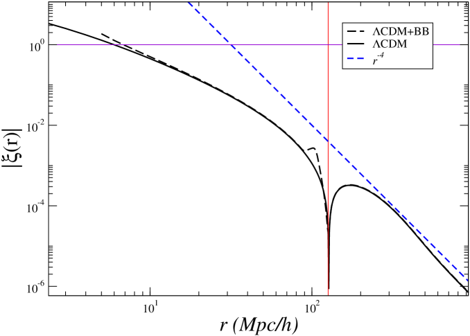
Before discussing whether the large scale structures identified in galaxy catalogs are compatible with the prediction of the standard LCDM cosmology, let us briefly discuss which, are the main features of the galaxy two-point correlation function $\xi(r)$ according to this model (see Fig.1). There are three different regimes and three different length scales $r_{0},r_{c}$ and $r_{bao}$ Gabrielli et al., (2002); Sylos Labini and Vasilyev, (2008); Sylos Labini et al., 2009e . For $r>r_{0}$ the behavior is fixed by the physics of the early universe, being thus an imprint of the initial conditions. (i) On scales smaller than $r_{0}$, where $\xi(r_{0})=1$, matter distribution is characterized by strong clustering; i.e. $\xi(r)\gg 1$, about which little is known analytically and which is generally constrained by N-body simulations where it is typically found that, for $r<r_{0}$, $\xi(r)\sim r^{-\gamma}$ with $\gamma\approx 1.5$ (ii) The second length scale is such that $\xi(r_{c})=0$, and it is located at $r_{c}\gg r_{0}$ Gabrielli et al., (2002). In the range of scales $r_{0}<r<r_{c}$, $\xi(r)$ is characterized by small-amplitude positive correlations, which rapidly decay to zero when $r\rightarrow r_{c}$. The third length scale $r_{bao}$ is located on scales of the order of $r_{c}$. This is the real-space scale corresponding to the baryon acoustic oscillations (BAO) at the recombination epoch. (iii) Finally in the third range of scales, namely for $r>r_{c}$, $\xi(r)$ is characterized by a negative power-law behavior, i.e. $\xi(r)\sim-r^{-4}$ Gabrielli et al., (2002, 2005). Positive and negative correlations are exactly balanced in such a way that $\int_{0}^{\infty}\xi(r)d^{3}r=0$. This is a global condition on the system fluctuations, which corresponds to the super-homogeneous nature of the matter distribution Gabrielli et al., (2002, 2005); i.e., that this characterized by a sort of stochastic order and by fluctuations that are depressed with respect to a purely uncorrelated distribution of matter (i.e. white noise). This corresponds to the linear behavior of the matter power spectrum as a function of the wave-number $k$ for $k\rightarrow 0$ (named the Harrison-Zeldovich tail), and it characterizes not only the LCDM model but all models of density fluctuations in the framework of the Friedmann-Robertson-Walker metric Gabrielli et al., (2002, 2005). Roughly, structures correspond to positive correlations, while negative correlations correspond to under-densities; thus the length-scale $r_{c}$ can be regarded as an upper limit to the spatial extension of structures in these models.

To summarize: on large enough scales $r>r_{0}\approx 10$ Mpc/h the predicted density field must be uniform and weakly correlated (and thus self-averaging — see below). In these models, on large enough scales, fluctuations are small and thus gravitational clustering in an expanding universe gives a simple prediction, as in the linear regime initial fluctuations are only linearly amplified during the growth Durrer et al., (2003); Sylos Labini and Vasilyev, (2008). Correspondingly the probability density function (PDF) of fluctuations remains substantially Gaussian. Indeed, the central limit theorem can be broken when correlations are long-ranged and strong Gabrielli et al., (2005), while these models predict weak positive correlations beyond 10 Mpc/h and up to 150 Mpc/h and very weak negative correlations for $r>150$ Mpc/h.

Figure 1: Absolute value of the two-point correlation function for the $\Lambda$CDM model and for the same model with the baryonic bump (BB) at $\sim$ 100 Mpc/h (adapted from Sylos Labini and Vasilyev, (2008)). A reference line with power law index $-4$ is reported to illustrate the behavior for $r>150$ Mpc/h where the correlation function becomes negative.

3 Recent results on galaxy correlations

There is an extensive literature on the measurement galaxy correlations properties; here we briefly review some recent results which are useful to point out the status of the art in the field (we refer the interested reader to Sylos Labini et al., 2009a ; Sylos Labini et al., 2009b ; Sylos Labini et al., 2009c ; Sylos Labini et al., 2009d ; Sylos Labini et al., 2009e for more details). Few years ago Eisenstein et al. Eisenstein et al., (2005) determined the galaxy two-point correlation function in a preliminary luminous red galaxy (LRG) sample of the Sloan Digital Sky Survey (SDSS) data release 3 (DR3). They found that $r_{0}\approx 15$ Mpc/h, $r_{bao}\approx 110$ Mpc/h and $r_{c}\approx 150$ Mpc/h, thus claiming for an overall agreement with the LCDM prediction and for a positive detection of the scale $r_{bao}$ at about 110 Mpc/h. More recently other authors Cabré and Gaztañaga, (2008); Martínez et al., (2009); Kazin et al., (2009) measured the same estimator of the correlation function in the LRG-DR6 sample and in the LRG-DR7 sample. They found that $r_{c}\approx 200$ Mpc/h and that $r_{boa}\approx 100$ Mpc/h, although they also showed, by considering many realizations of mock galaxy catalogs, that the expected variance of the model is large enough that the observed baryonic acoustic peak and larger scale signal are only consistent with LCDM at the 1.5$\sigma$ level. In addition Martinez et al. Martínez et al., (2009) measured that $r_{c}\approx 50$ Mpc/h in the Two Degree Field Galaxy Redshift Survey (2dFGRS) samples; they claimed that $r_{bao}$ is detectable when the correlation function is negative. However this is not what one expects in the context of the LCDM model where, as discussed above, the zero point of the correlation function must be a single scale for any type of objects. Indeed both linear gravitational clustering, and biasing (i.e., threshold selection) the density field give rise to a linear amplification of the amplitude of $\xi(r)$ Sylos Labini and Vasilyev, (2008); Sylos Labini et al., 2009e .

In summary different authors found, in different samples, different values for the three scales $r_{0},r_{c},r_{bao}$. These results are puzzling as the model gives an unambiguous prediction for the scales $r_{c}$ and $r_{bao}$, leaving however undetermined, but in the range [5,15] Mpc/h, the scale $r_{0}$. This latter behavior is generally ascribed to a luminosity selection effect — luminosity bias. A little discussion is deserved to the problem of bias and variance in estimators, which can instead be a major issue in these analyses Sylos Labini and Vasilyev, (2008); Sylos Labini et al., 2009e .

There have been published other very puzzling results which seem to be in contrast with the above mentioned results. For instance, Loveday Loveday, (2004), by measuring the redshift-dependent luminosity function and the comoving radial density of galaxies in the SDSS-DR1, found that the apparent number density of bright galaxies increases by a factor $\approx$ 3 as redshift increases from $z=0$ to $z=0.3$ Loveday, (2004). To explain these observations a significant evolution in the luminosity and/or number density of galaxies at redshifts $z<0.3$ has then been proposed Loveday, (2004). However an independent test has not been provided to support such a conclusion. Independently of the origin of this density growth, it remains that major issue that the density is not constant and thus its determination inside this sample is very ambiguous. As the correlation function $\xi(r)$ measures the amplitude and the scale dependence of correlations between density fluctuations normalized to the sample value of the density, if this quantity is not well-defined and determined with a small error, there can be substantial systematic (i.e. volume-dependent) effects on its estimation.

Another puzzling observation is represented by a CCD survey of bright galaxies within the Northern and Southern strips of 2dFGRS Colless et al., (2001). This shows conclusive evidences of fluctuations of $\sim 30\%$ in galaxy counts as a function of apparent magnitude busswell03 (see also frith03 ; frith06 for similar observations in other galaxy samples). Further since in the angular region toward the Southern galactic cap a deficiency, with respect to the Northern galactic cap, in the counts below magnitude $\sim 17$ was found, persisting over the full area of the APM and APMBGC catalogs, this would be an evidence that there is a large void of radius of about $150$ Mpc/h implying that there are spatial correlations extending to scales larger than the scale detected by the 2dFGRS correlation function norbergxi01 ; norbergxi02 . Indeed, by considering the two-point correlation function, and thus by normalizing the amplitude of fluctuations to the estimation of the sample density, the length-scale $r_{0}\approx 6-8$ Mpc/h was derived norbergxi01 ; norbergxi02 . Structures and fluctuations at scales of the order of 100 Mpc/h or more are at odds with the prediction of the concordance model of galaxy formation busswell03 ; frith03 ; frith06 , while the small value of the correlation length is indeed compatible.

Summarizing the current observational situation: there are evidences that galaxy distribution exhibits large amplitude fluctuations on scales of $\sim 100$ Mpc/h. On the other hand there are many results showing that $r_{0}\approx 10$ Mpc/h, while there is a substantial indetermination on the value of $r_{c}$, although in the very large volumes of the LRG samples it was found $r_{c}\approx 200$ Mpc/h. In what follows we try to clarify this puzzling situation, i.e. the coexistence of the small typical length scale $r_{0}$ measured by the two-point correlation function analysis with the large fluctuations in the galaxy density field on large scales as measured by the simple galaxy counts. The problem is that because of the large fluctuations in galaxy counts, the estimation of the sample density is not stable and thus one must critically consider the significance of the normalization of fluctuations amplitude to the estimation of the sample density as used in the correlation analysis employed to measure the length scales $r_{0},r_{c}$ and $r_{bao}$.

4 Testing theoretical models against data

In evaluating whether a model (CDM) is consistent with the data, it should be shown that at least the main statistical properties of the model are indeed consistent with the data. There is a number of different properties which can one consider and which are useful to test the assumptions that have been used when one studies the consistence of a theoretical model with real data by only considering the behavior of $\xi(r)$. Namely the assumptions of (i) self-averaging (ii) uniformity (or spatial homogeneity). When, inside the given sample, the assumption (i) and/or (ii) are/is violated then the conclusion is that CDM model is not compatible with the properties of the data Sylos Labini et al., 2009a ; Sylos Labini et al., 2009b ; Sylos Labini et al., 2009d ; Sylos Labini et al., 2009c . In general little attention is deserved to these properties and one generally assumed that these are satisfied inside a given sample focusing directly on the behavior of $\xi(r)$ or that of its Fourier conjugate, the power spectrum. Indeed, the use of any statistical quantity which is normalized to some estimations of the sample density implicitly assume that a distribution, inside the given finite sample, is self-averaging and uniform.

In order to illustrate the problems underlying these assumptions, let us consider a simple one-dimensional density field. In Fig.2 (left panel) it is shown the case of one dimensional density field with small amplitude fluctuations. In red we report two examples of samples with finite spatial extension. In each of the two cases one measures the sample density $\overline{n}$ which is “close” to the asymptotic average density $\langle n\rangle$ (i.e., the ensemble average density or the average density measured in the infinite volume limit). The rate of the difference between $\overline{n}$ and $\langle n\rangle$ with scales is determined by the behavior of the two-point correlation function Gabrielli et al., (2005). A completely different situation is represented by the one-dimensional density field shown in Fig.2 (right panel). In this case the field is characterized by large fluctuations and the determination of the sample density $\overline{n}$ in different regions (red lines) does not give a useful information about $\langle n\rangle$.

Figure 2: Left panel: One dimensional density field with small amplitude fluctuations. Right panel: One dimensional density field with large amplitude fluctuations

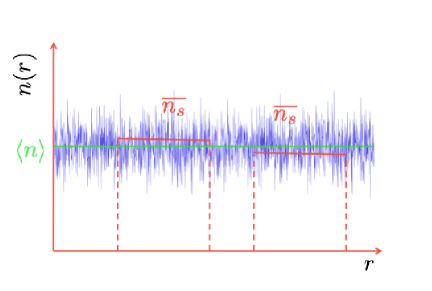
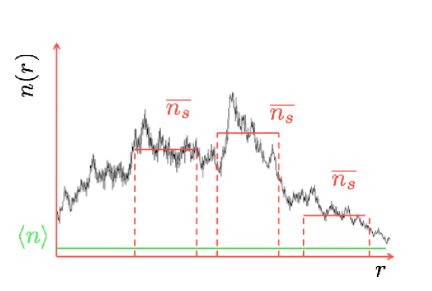
It is then clear that depending on the properties of the density field, one should adopt a certain statistical characterization or another. While in the case shown in the left panel of Fig.2 it is meaningful to normalize fluctuations to the sample estimate of the density, this becomes meaningless in the case shown in the right panel of Fig.2. Thus, in a finite sample one needs to set up a strategy to test the different assumptions used in the statistical analysis. To this aim one has to make a clear distinction between statistical quantities which are normalized to the sample average density and those which are not. If one wish to determine whether a statistically meaningful estimate of the average density is possible in the given samples, one should use statistical quantities that do not require the assumption of homogeneity inside the sample and thus avoid the normalization of fluctuations to the estimation of the sample average. These are thus conditional quantities, as for example the conditional density $n_{i}(r)$ from the $i^{th}$ galaxy, which gives the density in a sphere of radius $r$ centered on the $i^{th}$ galaxy. Conditional quantities are well-defined both in the case of homogeneous and inhomogeneous point distributions, as they require only local (i.e., not global) determination of statistical properties Sylos Labini et al., 2009d .

In general one should consider also another important complication. Statistical properties are determined by making averages over the whole sample volume Gabrielli et al., (2005). In doing so, one implicitly assumes that a certain quantity measured in different regions of the sample is statistically stable, i.e., that fluctuations in different sub-regions are described by the same probability density function (PDF). However it may happen that measurements in different sub-regions show systematic (i.e., not statistical) differences, which depend, for instance, on the spatial position of the specific sub-regions (see Fig.3).

Figure 3: One dimensional density field with large fluctuations: this density field is not self-averaging inside the considered sample, as the local density varies in a systematic way.

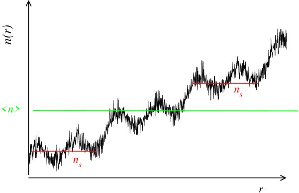
In this case the considered statistic is not statistically stationary in space, the PDF systematically differs in different sub-regions and its whole-sample average value is not a meaningful descriptor Gabrielli et al., (2005). In general such systematic differences may be related to two different possibilities: (i) that the underlying distribution is not translationally and/or rotationally invariant; (ii) that the volumes considered are not large enough for fluctuations to be self-averaging Sylos Labini et al., 2009c ; Sylos Labini et al., 2009d .

For this reason, our first aim is to study whether galaxy distribution is self-averaging by characterizing conditional fluctuations. If the distribution is self-averaging, then one can consider whole-sample conditional average quantities and study the possible transition from non-uniformity to uniformity. This can be achieved by characterizing the behavior of, for instance, the conditional density. If the distribution is uniform, or becomes uniform at a certain scale smaller than the sample size, one can characterize the (residual) correlations between density fluctuations by studying the standard two-point correlation function. Therefore the consideration of $\xi(r)$ is the last point in this list, and it is appropriate only if one has proved that the distribution is self-averaging and uniform inside the given sample. We make similar tests in the real samples and in the mock catalogs which represent the model predictions. In this way we test whether large scale structures identified in galaxy catalogs are compatible with the prediction of the standard LCDM cosmology,

5 Statistical properties of galaxy distribution in the 2dFGRS and SDSS samples

The main stochastic variable which we consider and of which we determine statistical properties is the conditional number of points in spheres mentioned above. Namely we compute for each scale $r$ the $\{N_{i}(r)\}_{i=1...M}$ determinations of the number of points inside a sphere of radius $r$ centered on the $i^{th}$ galaxy Sylos Labini et al., 2009d . The random variable $N_{i}(r)$ depends thus on the scale $r$ and on the spatial position of the sphere’s center; we can express the $i^{th}$ sphere center coordinates with its radial distance $R_{i}$ and with its angular coordinates $\vec{\alpha}_{i}=(\eta_{i},\lambda_{i})$. Thus, in general, we can write

$$N_{i}(r)=N(r;R_{i},\vec{\alpha}_{i})\;.$$ (1)

When we integrate over the angular coordinates $\vec{\alpha}_{i}$ for fixed radial distance $R_{i}$ we have that $N_{i}(r)=N(r;R_{i})$, i.e. it depends on two variables the length-scale of the sphere $r$ and the distance-scale of the $i^{th}$ sphere center $R_{i}$ and thus it has been called the scale-length analysis Sylos Labini et al., 2009d ; Sylos Labini et al., 2009c .

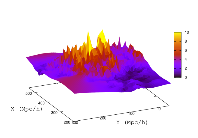
In Fig.4 we show the three-dimensional representation of $N(r;R_{i})$ in a sample of the SDSS-DR6. On the $X$ and $Y$ axis it is reported the coordinate of the center of a sphere of radius $r=20$ Mpc/h (centered on a galaxy) and on the $Z$ axis the number of galaxies inside it, normalized to its average value in this sample. The mean thickness of this slice is about 50 Mpc/h. Large fluctuations in the density field traced by the SL analysis $N_{i}(r;R)$ are located in the correspondence of large scale structures. The information contained in the $N(r;R_{i})$ data allow one to quantitatively determine the properties of these structures in an unambiguous way.

Figure 4: Three dimensional representation of the SL analysis with $r=10$ Mpc/h in a SDSS sample (adapted from Sylos Labini et al., 2009d ).

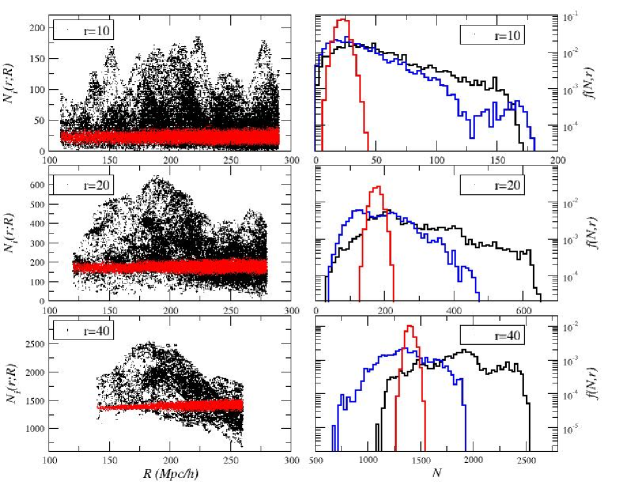
For instance we can determine the PDF of conditional fluctuations. An example is reported in Fig.5. In this sample, extracted from the SDSS Sylos Labini et al., 2009d , the SL analysis detects large density fluctuations without a clear radial-distance dependent trend. Correspondingly the PDF has a regular shape characterized by a peak with a long $N$ tail and it is sufficiently statistically stable in different non-overlapping sub-samples of equal volume. This occurs except for the largest sphere radii, i.e., for $r>$30 Mpc/h. The conclusion is that conditional fluctuations in this sample are self-averaging for $r<30$ Mpc/h, while they are not self-averaging for $r>30$ Mpc/h because of the limited sample volumes. These fluctuations determine relative variations larger than unity in the estimation of the average density, in the deepest samples, in spheres of radius $r=100$ Mpc/h. The homogeneity scale must be $>100$ Mpc/h, the largest sphere radius available in SDSS-DR6. The behavior of the PDF can a priori be determined also by selection effects and not only by fluctuations. However we tested that in the SDSS known selection effects do not give a relevant contribution: we used volume-limited samples and we made several tests to determine the importance of cosmological corrections, such as different magnitude-distance relations (i.e., different cosmological parameters), K-corrections and evolutionary corrections Sylos Labini et al., 2009d . It is interesting to note that for $r<20$ Mpc/h the PDF of fluctuations displays a “fat tail”, and in this case an excellent fit is given by the Gumbel distribution Antal et al., (2009).

Actually, in the largest samples of SDSS-DR7 we found Antal et al., (2009) that over a large range of scales, both the average conditional density and its variance show a nontrivial scaling behavior. The average conditional density depends, for $10\leq r\leq 80$ Mpc/h, only weakly (logarithmically) on the system size. Indeed, contrary to the case of SDSS-DR6, in the larger sample volumes of DR7 fluctuations are self-averaging up to $\sim 80$ Mpc/h. Correspondingly, we find that the density fluctuations follow the Gumbel distribution of extreme value statistics. This distribution is clearly distinguishable from a Gaussian distribution, which would arise for a homogeneous spatial galaxy configuration. We concluded that there are similarities between the galaxy distribution and critical systems of statistical physics, which can display the same two features when correlations are long-ranged. Analogously in the 2dFGRS we found that the average conditional density presents scaling behavior up to $\sim 30$ Mpc/h and the PDF of conditional fluctuations show “fat tails” Sylos Labini et al., 2009a ; Sylos Labini et al., 2009b .

Previous analyses of these galaxy catalogs, e.g., considered sample averaged statistics without quantitatively testing whether a significant bias could affect the results. For instance the estimator of the most commonly used statistics, the two-point correlation function, can be written as Gabrielli et al., (2005)

$$\xi(r)+1\equiv\frac{\langle n(r)n(0)\rangle}{\langle n\rangle^{2}}=\lim_{V\rightarrow\infty}\frac{\overline{N(r,\Delta r)}}{V(r,\Delta r)}\cdot\frac{V}{N}\;,$$ (2)

where in the second equality we have considered the finite sample estimator (in the ensemble average sense the symbol $\overline{N}$ should be replaced by $\langle N\rangle$). The first ratio in the r.h.s. of Eq.2 is the differential average conditional density, i.e., the number of galaxies in shells of thickness $\Delta r$ averaged over the whole sample, divided by the volume $V(r,\Delta r)$ of the shell. The second ratio in the r.h.s. of Eq.2 is the average density estimated in a sample containing $N$ galaxies and with volume $V$. When measuring this function we implicitly assume, in a given sample, that: (i) fluctuations are self-averaging in different sub-volumes Gabrielli et al., (2005) (ii) the linear dimension of the sample volume is $V^{1/3}\gg\lambda_{0}$ Gabrielli et al., (2005), i.e., the distribution has reached homogeneity inside the sample volume. When the latter condition is not verified the $\xi(r)$ analysis is biased by systematic finite size effects even if fluctuations are self-averaging Gabrielli et al., (2005). These two assumptions can be tested directly by considering conditional fluctuations properties, or indirectly by studying finite-volume effects on $\xi(r)$ determinations. The result of the $\xi(r)$ analysis is however in general not conclusive (see Sect 4.8 of Sylos Labini et al., 2009d ). For instance, in order to test how estimator bias (e.g., the effect of the integral constraint) affects the results, one can consider samples with different volumes and study whether there is a convergence to a stable behavior, which was not found in the case of the LRG samples Sylos Labini et al., 2009e .

Figure 5: Left panels: From top to bottom the SL analysis a SDSS sample, with $r=10,20,40$ Mpc/h. The red dots correspond to an uncorrelated distribution (Poisson) in the same volume and with same number of points. Right panels: Probability density function of $N_{i}(r;R)$ in two non-overlapping sub-samples with equal volume (each half of the sample volume) at small and large $R$. While for $r=10,20$ Mpc/h the PDF (nearby sub-sample black line and faraway sub-sample blue line) is reasonably statistically stable, for $r=40$ Mpc/h there is a clear difference. The red line corresponds to the Poisson distribution: a Gaussian function gives very good fits for all $r$ (adapted from Sylos Labini et al., 2009d ).

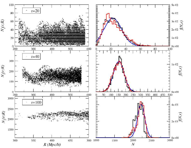
Let us now discuss the case of a mock galaxy catalogs. These are generated from N-body simulations of standard cosmological models springel05 , $N_{i}(r;R)$ does not show, for $r>10$ Mpc/h, large fluctuations or systematic trends as a function of $R$ (Fig.6). This is in agreement with the theoretical expectations based on the linear growth of perturbations in an expanding universe Sylos Labini et al., 2009d . Because in these artificial catalogs fluctuations are small and self-averaging, whole-sample averaged statistics are meaningful at all scales. Correspondingly the PDF rapidly converges to a Gaussian for $r>10$ Mpc/h. Thus mock catalogs, i.e. model predictions, are self-averaging at all scales and uniform for $r>10$ Mpc/h Sylos Labini et al., 2009d , and therefore the mock galaxy distribution is qualitatively different from the real one. In agreement with our results we note that Einasto et al., 2006a found that the fraction of very luminous (massive) super-clusters in real samples extracted from 2dFGRS and from the SDSS (Data Release 4), is more than ten times greater than in simulated samples. This again points toward a non-trivial disagreement between the galaxy distribution and the mock catalogs, stressing the fact that galaxy structures are more common in observations than in the model.

Figure 6: From top to bottom the SL analysis $N_{i}(r;R)$ for the mock sample VL2, with $r=20,40,100$ Mpc/h. Although for $r=20$ Mpc/h fluctuations are still important, they rapidly become small for larger radii without any signature of a radial-distance dependent trend. Right panels: Probability density function of $N_{i}(r;R)$ in two different non-overlapping sub-samples with equal volume (each half of the sample volume) at small (red line) and large (black line) $R$: the PDF is statistically stable for all $r$ and $R$. The blue line corresponds to a Gaussian fit.

6 Conclusions

We interpret the systematic differences found in the behavior of the PDF of conditional fluctuations as due to a systematic effect in the fact that sample volumes are not large enough for conditional fluctuations, filtered at such large scales, to be self-averaging, i.e. to contain enough structures and voids of large size to allow a reliable determination of average (conditional) quantities. We pointed out the problems related to the estimation of amplitude of fluctuations and correlation properties from statistical quantities which employ the normalization to the estimation of the sample average. As long as a distribution inside the given sample is not self-averaging, and thus not homogeneous, the estimation of the two-point correlation function is necessarily biased by strong finite size effects. Our results are incompatible with homogeneity at scales smaller than $\sim 100$ Mpc/h. While these results are at odds with LCDM predictions, they can be compatible, at least theoretically, with a several recent observations which also pose fundamental challenges to such a model.

For instance, Kashlinsky et al. Kashlinsky et al., (2008), by studying the fluctuations in the cosmic microwave background generated by the scattering of the microwave photons by the hot X-ray emitting gas inside clusters, have measured a coherent flow out to 300 Mpc/h with a fairly high amplitude of 600-$10^{3}$ km/sec. This is incompatible with the standard LCDM model predictions. Indeed, on such large scales the theoretical predictions are very simple, because in these models gravitational clustering is still linear at those scales as density fluctuations are small on large scales. Similarly Watkins et al. Watkins et al., (2008) estimated the bulk flow in all major peculiar velocity surveys finding that the data suggest that the bulk flow within a Gaussian window of radius 50 Mpc/h is 407 km/s. They noticed that this large-scale bulk motion indicates that there are significant density fluctuations on very large scales. Indeed, a flow of this amplitude on such a large scale is not expected in the LCDM model cosmology, for which the predicted one-dimensional r.m.s. velocity is about 110 km/s. Thus the same problem for the model predictions we found in the galaxy density field, are found also for the galaxy velocity field. They may have the same origin, namely the fact that there are galaxy structures which are too extended in space and have a too large amplitude to be compatible with the predictions of the standard model. In the case of the velocity field there is another important element: the velocity field is generated by all the mass and not only by the luminous component. Thus if the velocity field is so high on such large scales, this may imply that this is generated by the large scale inhomogeneities present in the overall mass distribution, i.e. luminous plus dark. The fact that the whole mass distribution is not homogeneous is compatible also with the results on the matter density field derived by gravitational lens observations, where very extended structures have been found Massey et al., (2007). Thus an important point which we aim to investigate in future works, concerns the characterizing of the gravitational field generated by galaxies. When a distribution is inhomogeneous important contributions to the gravitational force acting on a point can be due to faraway sources force . The relation between the large scale inhomogeneities of galaxy distribution and other observational data should be examined in detail. For instance a statistically significant anisotropy of the Hubble diagram at redshifts $z<0.2$ was discovered by Schwarz and Weinhorst, (2007). A local violation of statistical isotropy and homogeneity, which may very well happen when matter distribution is inhomogeneous Sylos Labini, (1994); Joyce et al., (2000), can be related to such findings. although it is not excluded that a systematic error in the observations or data analysis affect these results.

Finally, it is worth mentioning that Joyce et al. Joyce et al., (2000) pointed out that an inhomogeneous distribution, as a fractal, does not preclude the description of its gravitational dynamics in the framework of the Friedmann-Robertson-Walker solutions to general relativity. Indeed, the problem is often stated as being due to the incompatibility of a fractal with the Cosmological Principle, where this principle is identified with the requirement that the matter distribution be isotropic and homogeneous. This identification is in fact very misleading for a non-analytic and inhomogeneous structure like a fractal, in which all points are equivalent statistically, satisfying what has been called a Conditional Cosmological Principle Sylos Labini, (1994); Gabrielli et al., (2005). By treating the fractal as a perturbation to an open cosmology in which the leading homogeneous component is the cosmic background radiation one may get a simple explanation for the supernovae data which indicate the absence of deceleration in the expansion. This is indeed a very simplified theoretical model to interpret the SN data and the large scale inhomogeneities in framework of the Friedmann-Robertson-Walker metric.

References

- Huchra et al., (1983) J. Huchra, M. Davis, Latham D., and Tonry J., Astrophys.J.Suppl, 52, 89-119 (1983).
- Falco et al., (1999) E.F. Falco, et al., Pub.Astron.Soc.Pac., 111, 438-452 (1999).
- Giovanelli and Haynes, (1993) R. Giovanelli, and M.P. Haynes, Astronom.J. 105, 1271-1290 (1993).
- da Costa et al., (1988) L. da Costa, et al., Astrophys.J., 327, 544-560 (1988).
- Shectman et al., (1996) S. A. Shectman, et al., Astrophys.J., 470, 172-188 (1996).
- York et al., (2000) D. York, et al., Astronom.J. 120, 1579-1587 (2000).
- Colless et al., (2001) M. Colless , et al., Mon.Not.R.Acad.Soc, 328, 1039-1063 (2001).
- de Lapparent Huchra and Geller, (1986) V. de Lapparent, M.J. Geller, J.P. Huchra, Astrophys.J., 302, L1-L5 (1986).
- Geller and Huchra, (1989) M.J. Geller, J.P. Huchra Science, 246, 897-903 (1989).
- Gott et al., (2005) J.R. III Gott, , et al., Astrophys.J., 624, 463-484 (2005).
- Gabrielli et al., (2002) A. Gabrielli, M. Joyce, F. Sylos Labini, Phys.Rev., D65, 083523-1-083523-18 (2002).
- Sylos Labini and Vasilyev, (2008) F. Sylos Labini, N.L. Vasilyev, Astron.Astrophys. 477, 381-395 (2008).
- (13) F. Sylos Labini, N.L. Vasilyev, Yu.V. Baryshev, M. López-Corredoira, Astron.Astrophys., 505, 981-990 (2009)
- Gabrielli et al., (2005) A. Gabrielli, F. Sylos Labini, M. Joyce and L. Pietronero “Statistical physics for cosmic structures” Springer-Verlag (2005).
- Durrer et al., (2003) R. Durrer, A. Gabrielli, M. Joyce, and F. Sylos Labini, Astrophys.J., 585, L1-L4 (2003).
- (16) F. Sylos Labini, N. L. Vasilyev, Y.V. Baryshev, Europhys.Lett. , 85 , 29002-p1-29002-p6, (2009).
- (17) F. Sylos Labini, N. L. Vasilyev, Y.V. Baryshev, Astron.Astrophys., 496, 7-23 (2009).
- (18) F. Sylos Labini, N. L. Vasilyev, L. Pietronero, Y.V. Baryshev, Europhysics Letters, 86, 49001-p1-49001-p6 (2009).
- (19) F. Sylos Labini, N. L. Vasilyev, Y.V. Baryshev, Astron.Astrophys., in the press arXiv:0909.0132 (2009).
- Eisenstein et al., (2005) D.J. Eisenstein, Astrophys.J., 633, 560-574 (2005).
- Cabré and Gaztañaga, (2008) A. Cabré, and E. Gaztañaga, Mon.Not.R.Acad.Soc, 396, 1119-1131 (2009).
- Martínez et al., (2009) V.J Martínez, et al. Astrophys.J., 696, L93-L97 (2009).
- Kazin et al., (2009) E. Kazin et al., arXiv:0908.2598 (2009).
- Loveday, (2004) J. Loveday, Mon.Not.R.Acad.Soc, 347, 601-606 (2004).
- (25) G.S. Busswell, et al., Mon.Not.R.Acad.Soc 354, 991-1004 (2004).
- (26) W.J. Frith, et al., Mon.Not.R.Acad.Soc, 345, 1049-1056 (2003).
- (27) W.J. Frith, et al., Mon.Not.R.Acad.Soc, 371, 1601-1609 (2006).
- (28) E. Norberg, et al., Mon.Not.R.Acad.Soc, 328, 64-70 (2001).
- (29) E. Norberg, et al., Mon.Not.R.Acad.Soc, 332, 827-838 (2002).
- Antal et al., (2009) T. Antal, F. Sylos Labini, N. L. Vasilyev, Y.V. Baryshev arXiv:0909.1507 (2009).
- (31) V. Springel, et al., Nature, 435, 629-636 (2005).
- (32) J. Einasto, et al., Astron.Astrophys., 459, L1-L4 (2006).
- Kashlinsky et al., (2008) A. Kashlinsky, et al., Astrophys.J., 686, L49-L52 (2008).
- Watkins et al., (2008) R. Watkins, H.A. Feldman, M.J. Hudson, Mon.Not.R.Acad.Soc, 392, 743-756 (2009).
- Massey et al., (2007) R. Massey, et al., Nature, 445, 286-290 (2007).
- (36) A. Gabrielli, F. Sylos Labini, & S. Pellegrini, Europhys.Lett., 46, 127-133 (1999).
- Schwarz and Weinhorst, (2007) D.J. Schwarz, B. Weinhorst, Astron.Astrophys., 474,717-729 (2007).
- Joyce et al., (2000) M. Joyce, P. W. Anderson, M. Montuori, L. Pietronero and F. Sylos Labini, Europhys.Letters, 50, 416-422 (2000).
- Sylos Labini, (1994) F. Sylos Labini, Astrophys.J., 433, 464-467 (1994).