Galaxy cluster searches by photometric redshifts in the CFHTLS

Abstract

Context. Counting clusters is one of the methods to constrain cosmological parameters, but has been up to now limited both by the redshift range and by the relatively small sizes of the homogeneously surveyed areas.

Aims. In order to enlarge publicly available optical cluster catalogs, in particular at high redshift, we have performed a systematic search for clusters of galaxies in the Canada France Hawaii Telescope Legacy Survey (CFHTLS).

Methods. We considered the deep 2, 3 and 4 CFHTLS Deep fields (each 1$\times$1 deg²), as well as the wide 1, 3 and 4 CFHTLS Wide fields. We used the Le Phare photometric redshifts for the galaxies detected in these fields with magnitude limits of i’=25 and 23 for the Deep and Wide fields respectively. We then constructed galaxy density maps in photometric redshift bins of 0.1 based on an adaptive kernel technique and detected structures with SExtractor at various detection levels. In order to assess the validity of our cluster detection rates, we applied a similar procedure to galaxies in Millennium simulations. We measured the correlation function of our cluster candidates. We analyzed large scale properties and substructures, including filaments, by applying a minimal spanning tree algorithm both to our data and to the Millennium simulations.

Results. We have detected 1200 candidate clusters with various masses (minimal masses between 1.0 10¹³ and 5.5 10¹³ and mean masses between 1.3 10¹⁴ and 12.6 10¹⁴ M_⊙) in the CFHTLS Deep and Wide fields, thus notably increasing the number of known high redshift cluster candidates. We found a correlation function for these objects comparable to that obtained for high redshift cluster surveys. We also show that the CFHTLS deep survey is able to trace the large scale structure of the universe up to z$\geq$1. Our detections are fully consistent with those made in various CFHTLS analyses with other methods. We now need accurate mass determinations of these structures to constrain cosmological parameters.

Conclusions. We have shown that a search for galaxy clusters based on density maps built from galaxy catalogs in photometric redshift bins is successful and gives results comparable to or better than those obtained with other methods. By applying this technique to the CFHTLS survey we have increased the number of known optical high redshift cluster candidates by a large factor, an important step towards using cluster counts to measure cosmological parameters.

1 Introduction

The beginning of the 21st century is an exciting period for cosmological studies. Several methods now allow to put strong constraints on cosmological parameters. We can for example reconstruct Hubble diagrams (supernovae or tomography) or use directly the primordial fluctuation spectrum. In addition, the cluster count technique is probably the oldest one (see e.g. Gioia et al., 1990). Up to now this technique was penalized by the redshift range of detected clusters, which was too low to make the difference between flat and open universes. Distant cluster surveys have also been mainly conducted in areas too small or with inhomogeneous selection functions. Besides cluster mass knowledge, this technique requires indeed large fields of view of several dozen square degrees to provide large numbers of cluster detections at z$\geq$1 (e.g. Romer et al. 2001). Recent X-ray cluster surveys are beginning to produce cluster catalogs at high z (e.g. the XMM-LSS survey, Pierre et al., 2007) and it is the goal of the present paper to contribute to the production of similar large cluster catalogs based on optical Canada France Hawaii Telescope Legacy Survey data.

The Canada-France-Hawaii Telescope Legacy Deep and Wide Surveys (CFHTLS-D and CFHTLS-W) respectively explore solid angles of 4 deg² and 171 deg² of the deep Universe, each in 4 independent patches (http://www.cfht.hawaii.edu/Science/CFHLS/). For both surveys, observations are carried out in five filters ($u*,g^{\prime},r^{\prime},i^{\prime}$ and $z^{\prime}$) providing catalogs of sources that are 80% complete up to $i_{AB}$=26.0 (CFHTLS-D) and $i_{AB}$=24.0 (CFHTLS-W) (Mellier et al 2008, http://terapix.iap.fr/cplt/oldSite/Descart/CFHTLS-T0005-Release.pdf). The CFHTLS-W, in particular, encloses a sample of about 20 10⁶ galaxies inside a volume size of $\sim 1$ Gpc³, with a median redshift of z$\sim 0.92$ (Coupon et al 2009). According to the standard cosmological model, the CFHTLS-W (W1, W2, W3, and W4 herafter) is then expected to contain 1000 to 5000 clusters of galaxies with accurate photometric redshifts, most of them in the $0.6<z<1.5$ range. Likewise, the CFHTLS-D (D1, D2, D3, and D4 hereafter) should contain 50 to 200 clusters, with a significant fraction at higher redshift than the CFHTLS-W. The two surveys are therefore complementary data sets. They can produce together two homogeneous optically selected samples of clusters of galaxies that can be reliably compared and used jointly to explore the mass function, the abundance of clusters of galaxies and the evolution of cluster galaxy populations as a function of lookback time.

The construction of homogeneous catalogs of optically selected clusters of galaxies is not, a simple task. Early searches for clusters of galaxies in the CFHTLS were performed by Olsen et al. (2007) based on a matched filter detection algorithm applied to the Deep fields (see also the recent paper by Grove et al. 2009). Galaxy density maps combined with photometric redshift catalogs were considered by Mazure et al. (2007) in the D1 field. Lensing techniques were also employed to detect massive structures in the CFHTLS (e.g. Cabanac et al. 2007, Gavazzi $\&$ Soucail 2007, Bergé et al. 2008). Other cluster studies based on the CFHTLS data (e.g. the CFHTLS-CARS survey: Erben et al. 2009, Hildebrandt et al. 2009) and based for part of them on the red sequence in the color magnitude diagram are also in progress.

We present here a systematic search for galaxy clusters in the D2, D3 and D4 Deep fields (the D1 field was already analyzed by Mazure et al. 2007), as well as in the regions of the W1, W3 and W4 Wide fields available in the T0004 release. Our approach is based on photometric redshifts computed for all the galaxies extracted in each field (Coupon et al. 2009). In this way, we take into account the full color information and not only two bands as for example in red sequence searches. We divided the galaxy catalogs in slices of 0.1 in redshift, each slice overlapping the previous one by 0.05, and built density maps for each redshift slice. Structures in these density maps were then detected with the SExtractor software in the different redshift bins. We applied the same method to similar size mock samples built from the Millennium simulation, in order to estimate the reliability of our detections. We measured the clustering properties of our catalog. We then analyzed substructuring and filamentary large scale properties by applying a minimum spanning tree algorithm both to our data and to the Millennium simulation.

In this paper we assume H₀ = 70 km s^-1 Mpc^-1, $\Omega_{m}$=0.3, $\Omega_{\Lambda}$=0.7. All coordinates are given at the J2000 equinox and magnitudes are in the AB system.

2 Searching for clusters in the CFHTLS

A full description of the method applied to the D1 field is given in Mazure et al. (2007) and we adopt here the same method, which we briefly summarize below. We will not redo the D1 analysis because the D1 photometric redshifts in Mazure et al. (2007) have very similar quality compared to the present data. D1 cluster detections will only be considered for an internal crosscheck with the W1 detections of the present paper.

2.1 Photometric redshifts

We used the public photometric redshift catalogs from the CFHTLS data release T0004 (available at http://terapix.iap.fr/) in the D2, D3, D4, W1, W3 and W4 fields. The regions we selected inside the wide fields and covered by T0004 are mosaics of 19, 4 and 11 Megacam fields for W1, W3 and W4 respectively. In order to avoid incompleteness effects and strong systematic biases in photometric redshift computations, the catalogs were limited to i’=25 and 23 for the Deep and Wide fields respectively. This is slightly deeper than the recommended cuts of Coupon et al. (2009) but proved to not be a problem in our analysis.

Our approach is based on photometric redshifts, which can be estimated with good precision up to z$\sim$1.5 (Coupon et al. 2009) thanks to the optimal wavelength coverage achieved by the u*g’r’i’z’ CFHTLS data. Photometric redshifts were computed for all the objects in the CFHTLS galaxy catalogs with the Le Phare software developed by S. Arnouts and O. Ilbert (Ilbert et al. 2006; also see http://www.ifa.hawaii.edu/ĩlbert/these.pdf.gz, pages 50 and 142). Details of this computation are given in Mellier et al. (2008). Briefly, these photometric redshifts were computed with a large set of templates, covering a broad domain in parameter space (see Coupon et al. 2009 for a full description of the method and sample). Spectroscopic redshifts from the VVDS (e.g. LeFèvre et al. 2004) were used to optimize the photometric redshift estimates. This step is extensively described by Coupon et al. (2009) and the process consists in shifting the magnitude zero points until the difference between photometric and spectroscopic redshifts is minimized. These shifts were all lower than 0.1 magnitude, see Table 2 of Coupon et al. (2009). The resulting statistical errors (including the $1+z$ dependence) on the photometric redshifts are also given in Coupon et al. (2009). For example in the W1 field, they continuously increase (between i’=20.5 and i’=24) from 0.025 to 0.053. At our limiting magnitude of i’=23, the redshift statistical error is 0.043. Deep fields have nearly constant redshift statistical errors of the order of 0.026 (maximum is 0.028) for i’ magnitudes between 20.5 and 24.

We selected galaxies with photometric redshifts included in the range $0\leq z\leq 1.5$ for the Deep fields and $0\leq z\leq 1.2$ for the Wide fields.

For each CFHTLS field and subfield, we give in Table 1 the numbers of galaxies taken into account. This table will be useful for comparisons with future data releases.

Table 1: Number of galaxies in each CFHTLS field and subfield we studied. The considered magnitude limit is i’=23 for the wide fields and i’=25 for the deep fields.

Field	Subfield	Coordinates	Nb of galaxies
D2		100000+021220	376224
D3		141754+523031	500307
D4		221531-174405	458296
W1	1	021410-041200	221291
W1	2	021410-050800	216063
W1	3	021800-041200	218959
W1	4	021800-050800	237444
W1	5	021800-060400	221110
W1	6	022150-041200	224493
W1	7	022150-050800	205990
W1	8	022150-060400	218958
W1	9	022539-041200	228258
W1	10	022539-050800	195797
W1	11	022539-060400	177252
W1	12	022929-041200	181313
W1	13	022929-050800	201348
W1	14	022929-060400	183899
W1	15	022929-070000	195285
W1	16	023319-041200	220113
W1	17	023319-050800	198918
W1	18	023319-060400	200125
W1	19	023319-070000	190473
W3	1	135955+523831	241036
W3	2	140555+523831	226221
W3	3	141154+523831	208163
W3	4	141201+514231	204033
W4	1	220930+002300	231078
W4	2	220930-003100	204257
W4	3	221318+002300	235100
W4	4	221318-003100	230770
W4	5	221318+011900	210846
W4	6	221706+002300	207861
W4	7	221706-003100	171636
W4	8	221706+011900	213383
W4	9	222054+002300	197228
W4	10	222054-003100	215437
W4	11	222054+011900	221290

2.2 Density maps

In order to obtain results directly comparable with those previously obtained by Mazure et al. (2007), we applied the same procedure. For each field, galaxy catalogs were built in running slices of 0.1 in redshift (see also Mazure et al. 2007), displaced by 0.05 (i.e. the first slice covers redshifts 0.0 to 0.1, the second 0.05 to 0.15 etc.). We assumed the most likely photometric redshift for each object in order to assign it to a redshift slice. Density maps were then computed for each redshift slice, based on an adaptative kernel technique described in Mazure et al. (2007). The highest redshift slices were 1.30-1.40 and 1.35-1.50 for the Deep fields, and 1.05-1.15 for the Wide fields. An example of density map obtained is displayed in Fig. 1.

Figure 1: Density maps for the D2 field for the z=0.65-0.75 redshift bin. Two clusters are detected at S/N$\geq$6.

The SExtractor software (Bertin & Arnouts 1996) was then applied to the galaxy density maps to detect structures at pre-defined significance levels (called hereafter S/N) of $2\sigma_{S}$, $3\sigma_{S}$, $4\sigma_{S}$, $5\sigma_{S}$ and $6\sigma_{S}$ (where $\sigma_{S}$ is the SExtractor detection threshold).

The structures were then assembled in larger structures (called $detections$ in the following) using a friends-of-friends algorithm, as in Mazure et al. (2007). We assigned to a $detection$ the redshift of its highest S/N component.

We had made several experimentations for the Mazure et al. (2007) preliminary work, and found that the 0.1 redshift width of most of the studied slices was the best compromise between the redshift resolution and the possible dilution in the density signal due to photometric redshift uncertainties. We chose to keep the slice width larger than the maximal photometric redshift 1$\sigma$ uncertainty. For the wide fields, assuming the worse possible photometric redshift statistical error of 0.043$\times$$(1+z)$ (for i’=23, see Coupon et al. 2009) leads to a 1$\sigma$ error of 0.09 at z=1.15 (upper limit in redshift for the wide field analyses). For the deep fields, assuming a redshift statistical error lower than 0.028$\times$$(1+z)$ leads to a 1$\sigma$ error of 0.07 at z=1.5. Both values are lower than the 0.1 slice width we choose.

By definition of a Gaussian function, $\sim 32\%$ of the objects will have a true redshift differing by more than 1$\sigma$ from the most likely photometric redshift. This means that in the worse case (at the limiting magnitude and for the higher allowed redshift bin), slightly less than 30$\%$ of the objects (the slice width is slightly lower than the 1$\sigma$ value) will be assigned to a wrong redshift slice (mostly in the immediately higher or lower redshift slices). At lower redshifts and for brighter magnitudes, the percentage of such lost objects is low and is not a concern regarding our analysis. If we are close to the study limitations, it is then likely that the lost objects will be numerous enough to still be detected as part of a structure in the adjacent slices. The friends-of-friends algorithm described earlier will therefore associate these structures shifted in redshift to their true parent structure, therefore not significantly penalizing our analysis.

2.3 Modified Millennium catalogs

With this method, we obtained catalogs of galaxy cluster candidates in the various fields for a given significance level. In order to assess our detection levels we applied the same method to a modified version of the Millennium numerical simulation (e.g. Springel et al. 2005, http://www.mpa-garching.mpg.de/galform/virgo/millennium/ ), as follows:

- We started from semi-analytic galaxy catalogues obtained by applying the prescriptions of De Lucia $\&$ Blaizot (2007) to the dark-matter halo merging trees extracted from the Millennium simulation (Springel et al. 2005). The Millennium run distributes particles in a cubic box of size 500 h^-1 Mpc. The simulation was built with a $\Lambda$CDM cosmological model. For details on the semi-analytic model, we refer to De Lucia $\&$ Blaizot (2007) and reference therein. Note that this model uses the Bruzual $\&$ Charlot (2003) population synthesis model and a Chabrier (2003) Initial Mass Function (IMF) to assign luminosities to model galaxies. The $1\times 1$ deg² light cones were generated with the code MoMaF (Blaizot et al. 2005) and are complete in apparent magnitude up to I_AB=24. We used the 4 cones that had the most massive structures, more adequate for investigating cluster search.

- For each simulated galaxy, magnitude errors were computed in order to reproduce the (magnitude, magnitude error) mean relation obtained from the CFHTLS catalogues in all photometric bands. Magnitudes were then recomputed in order to reproduce the spread of the (magnitude, magnitude error) diagram assuming a gaussian distribution.

- We took into account occultation effects of background galaxies by foreground galaxies. For a given galaxy, we searched for brighter galaxies located in the foreground and large enough to occult the given object (included within the disk size of the foreground galaxy as defined in the Millennium simulation). If such occulting objects were found, we removed the occulted objects from the simulation. This removed 8$\%$ of the objects of the Millennium simulation.

- We took into account possible lensing effects which could potentially re-include occulted galaxies. For this, we estimated the image displacement of a galaxy due to a foreground massive object. Assuming an isothermal gravitational potential for the lens galaxy, the deflexion of a background object is then given by:

$$(\sigma_{v}/186.5\ km\ s^{-1})^{2}\times({\rm D}_{ls}/{\rm D}_{os})$$

in arcsec, where $\sigma_{v}$ is the velocity dispersion of the lens, D_ls the lens-source distance, and D_os the observer-source distance.

We computed $\sigma_{v}$ from the values of M₂₀₀ and r₂₀₀ given in the Millennium simulation.

Then, if the deflexion amplitude was larger than the occulting object disk radius, we re-included the lensed galaxy considered. This affected less than 1$\%$ of the Millennium simulation objects and the effect was therefore minor.

- We added noise to the true redshift values of the Millennium simulation in order to mimic the photometric redshift distribution computed in the CFHTLS Wide and Deep fields. This means that we produced one modified Millennium simulation in order to compare with the CFHTLS Deep fields and another one to compare with the CFHTLS Wide fields. The process was simply to compute the basic gaussian 1$\sigma$ error of the CFHTLS photometric redshifts as a function of redshift, as a function of magnitude, and as a function of magnitude uncertainty. This produced a cubic grid of $\sigma$’s with a resolution of 0.15 in redshift, 0.5 in magnitude, and 0.2 in magnitude uncertainty. This grid resolution is a good compromise between the computing time and the quality of the photometric redshifts. We then applied this grid to the true Millennium redshifts. These Millennium object redshifts were re-shuffled within a $\sigma$ characterized gaussian function according to the object redshift, magnitude, and magnitude error. Fig. 2 shows the resulting relations between true and photometric-like redshifts in the Millennium simulation .

Figure 2: True redshift values for the modified Millennium simulation versus photometric redshifts according to the CFHTLS criteria. Upper figure: Wide parameters, lower figure: Deep parameters.

- In order for the clusters detected in the Millennium simulations to be comparable to those in the Deep and Wide CFHTLS data, the catalogs of galaxies in the Millennium simulation were cut at R=25 and R=23 respectively. As previously described, galaxy catalogs were created in slices of photometric redshifts, density maps were computed, structures were identified with SExtractor, and the significance level was computed for each of them.

We note that several artificial galaxy concentrations in photometric redshifts appear in Fig. 2, mainly for the Wide survey characteristics. This is simply due to the characteristics of the CFHTLS data. We need to reproduce these biases in the Millenium simulations in order to properly quantify our false cluster detection rate in the CFHTLS data.

2.4 Detection rate assessments

We now need to estimate the $detection$ rate of our cluster detection method in the CFHTLS. This is complicated by the fact that the Millennium simulation has a very high spatial resolution compared to our galaxy density maps. This results in a non negligible multiplicity of Millennium halos in a single $detection$ made with our technique. For a given $detection$, we can usually find more than one halo in the Millennium simulation. We must therefore investigate each of our $detections$ in the Millennium simulation (152 for the Wide parameters and 179 for the Deep parameters respectively) to check how many Millennium halos can be associated.

For this purpose, and for a given $detection$:

- we computed the density of Millennium halos in the $detection$ as a function of their mass.

- for a given minimal mass, we compared this density to the mean density of Millennium halos included in the redshift range spanned by the $detection$ (and more massive than the given mass) but not spatially included in the $detection$.

If the ratio between these two densities was less than 0.1, we assumed that the density of halos present in a $detection$ was significantly different from the mean density at the same redshift, and therefore we had a significant mass concentration in our $detection$, i.e. our $detection$ was real. This means that we only keep $detections$ located in the 10$\%$ highest Millenium halo density regions. We did this exercise for several minimal Millenium halo masses (5 10¹², 8 10¹², 10¹³, 2 10¹³, 4 10¹³, and 6 10¹³ M_⊙). For clarity, we choose to express this with a significance parameter

$$p=100.\times(1.-{\rm densityratio})$$

. A $p$ value lower than 90$\%$ means that a $detection$ is fake. We considered a $detection$ as real if none of the values of $p$ (for various minimal masses) was lower than 90$\%$.

We give in Fig. 3 examples of the mass histograms of the Millennium halos present in two of our $detections$, one considered as a real $detection$, and the other considered as false.

Figure 3: Mass histograms of the Millennium halos (Wide survey characteristics) present in a real $detection$ (upper figure) and in a false $detection$ (lower figure). Each figure gives the number of halos included in the $detection$, the total and maximal mass of these halos (in log 10¹⁰ M_⊙), and 6 significance parameters $p$ for 6 different minimal masses (see text).

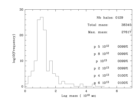
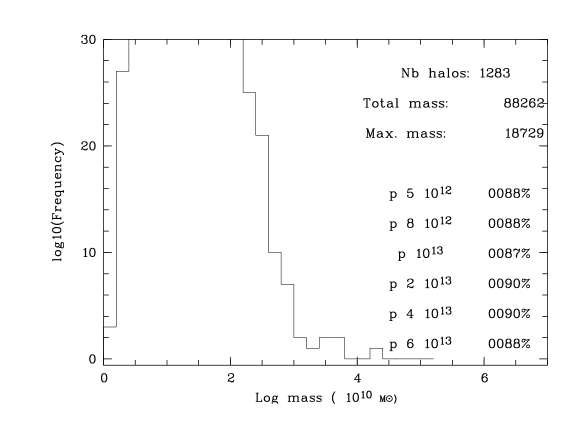
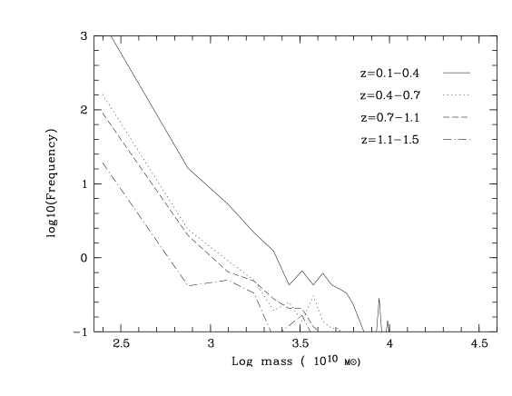
Fig. 4 gives the mean mass distributions of all the Millennium halos included in all our real $detections$ (CFHTLS Wide characteristics) as a function of mass for various $detection$ redshift bins.

Figure 4: Mass distributions of all the Millennium halos (CFHTLS Wide survey characteristics) included in real $detections$ as a function of mass for various $detection$ redshift bins.

Considering the criterion described above, we are able to give success rates in the detection process. Figs. 5 and 6 show the percentages of all Millennium halos identified with a real $detection$ as a function of mass.

Figure 5: Percentages of all Millennium halos included in real detections for the Wide survey characteristics as a function of redshift for different mass limits.

Figure 6: Percentages of all Millennium halos included in real detections for the Deep survey characteristics as a function of redshift for different mass limits.

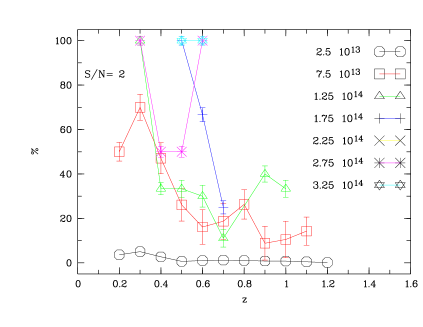
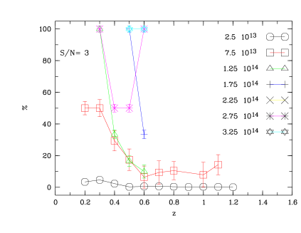
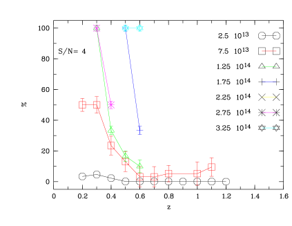
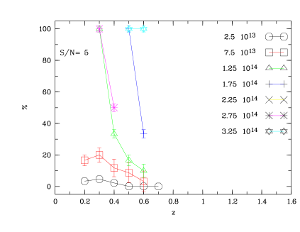
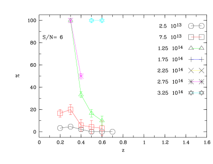
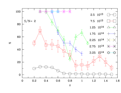
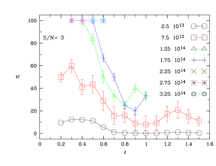
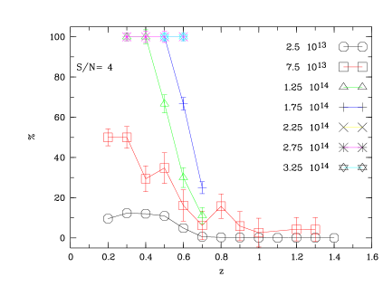
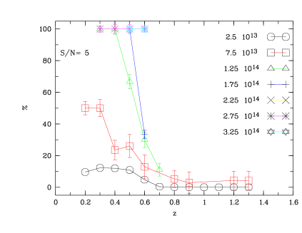
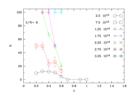
We see that for the Wide survey, we are only able to detect with a success rate greater than $\sim$20$\%$ the Millennium halos more massive than 7.5 10¹³ M_⊙. The detection rates become quite low at z$\geq$0.6-0.7. For the Deep survey, we also detect halos more massive than 7.5 10¹³ M_⊙ but up to z$\geq$0.9.

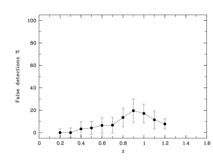
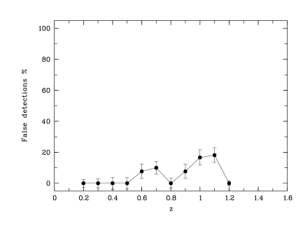
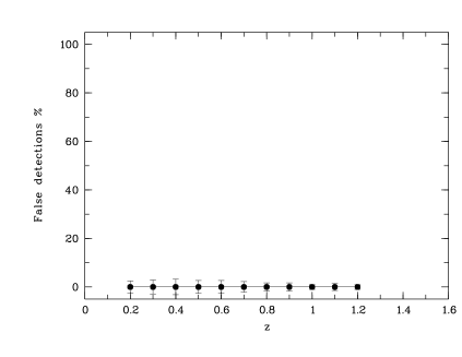
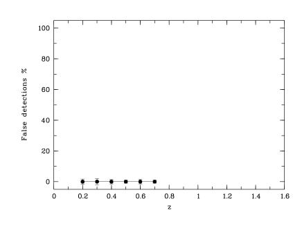
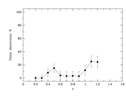
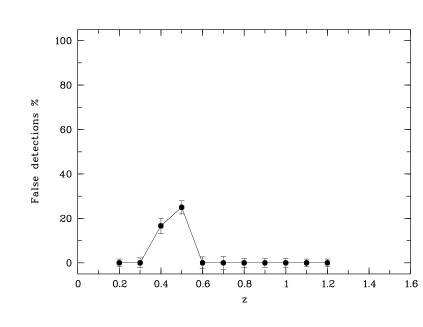
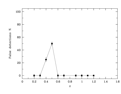
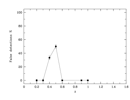
We give in Figs. 7 and 8 the percentages of fake $detections$ (following the criterion previously exposed) as a function of S/N detection and redshift for the Wide and Deep surveys. For the Wide survey, false $detection$ rates are basically null for S/N$\geq$4 and remain small for S/N$\leq$3 and z$\leq$0.8. For the Deep survey, false $detection$ rates are small whatever the S/N and for z$\leq$1. We note however an unexpected local increase of this rate at z$\sim$0.5 which is perhaps due to degeneracies in photometric redshift estimates producing artificial clustering signal for example because of the discreteness of the templates.

As a compromise between detection rate and false detection rate, we chose to not perform detections at S/N lower than 2. We could also have limited our catalogs to S/N$\geq$3 $detections$ to have a more robust sample. However, only about 10$\%$ of the S/N=[2;3[ $detections$ are fake and this percentage decreases to 6$\%$ for the S/N=[3;4[ $detections$. At the same time, the number of $detections$ is multiplied by $\sim$2.8 between S/N=[3;4[ and S/N=[2;3[. The number of real $detections$ therefore grows faster than the number of fake $detections$. Hence, considering S/N=[2;3[ $detections$ allows to include numerous real clusters as well as to keep fake $detections$ to a level lower than 10$\%$.

Figure 7: Percentages of fake $detections$ for the Wide survey characteristics as a function of redshift. From top to bottom: S/N of 2, 3, 4, 5, and 6.

Figure 8: Percentages of fake $detections$ for the Deep survey characteristics as a function of redshift. From top to bottom: S/N of 2, 3, 4, 5, and 6.

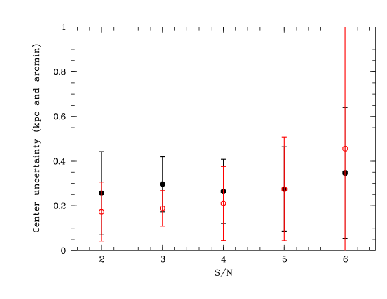
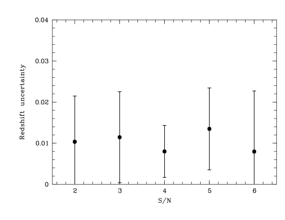
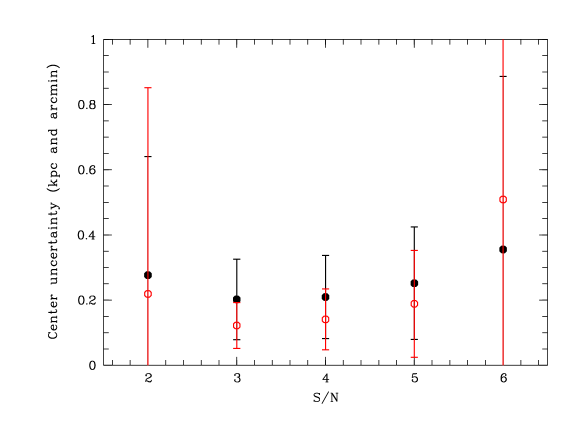
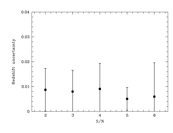
We now evaluate the coordinates and redshift precision of our $detections$. Using the Millennium simulation, we detected 97 candidate clusters at S/N=2, 27 at S/N=3, 16 at S/N=4, 4 at S/N=5, and 7 at S/N=6, which turned out to be massive halos in the Millennium simulation. With these detections, we estimated that the typical uncertainty on the candidate cluster coordinates was smaller than $\sim$1 arcmin or $\sim$0.5 kpc and smaller than 0.025 in redshift (see Figs. 9 and  10). We note that several massive Millennium halos can be identified with a single $detection$ (see also next section). To compute the statistics given in Figs. 9 and  10, we considered the Millennium halo which is the closest to the considered $detection$. We can note that the error bars tend to increase with S/N. For the top figure, this can be explained by the fact that at high S/N we detect massive clusters, which are often heavily substructured and therefore the definition of their center is not straightforward.

Figure 9: CFHTLS Wide-like Millennium simulation. Upper figure: shifts between true and estimated centers of the massive structures in the Millennium simulation as a function of the detection S/N. Open red circles with error bars are the values given in kpc, and filled black circles with error bars are the values given in arcmin. Lower figure: shifts between true and estimated redshifts of the massive structures in the Millennium simulation as a function of detection S/N.

Figure 10: CFHTLS Deep-like Millennium simulation. Upper figure: shifts between true and estimated centers of the massive structures in the Millennium simulation as a function of the detection S/N. Open red circles with error bars are the values given in kpc, and filled black circles with error bars are the values given in arcmin. Lower figure: shifts between true and estimated redshifts of the massive structures in the Millennium simulation as a function of detection S/N.

We also give a mass estimate based on the photometry. Each candidate cluster is detected at a given $S/N$. This detection threshold is a rough estimate of the cluster richness, being simply the net $flux$ of the source, i.e. the number of galaxies in the source diminished of the background level. The criterion is not precise enough (we only took detection thresholds in steps of 1) and luminosity function based richnesses would be better tracers of the total mass of the structures. However, this criterion allows to give a minimal mass for a detected structure. Table 2 therefore gives the relation between this detection threshold and the minimal cluster mass. We clearly see that when the detection threshold increases, the minimal mass also increases, both for the Deep and the Wide surveys.

Table 2: Relation between the SExtractor detection threshold and the minimal and mean (over all the associated Millennium halos) cluster masses.

SExtractor detection threshold	Minimal mass	Mean mass	Minimal mass	Mean mass
	Wide (M⊙)	Wide (M⊙)	Deep (M⊙)	Deep (M⊙)
2	1.0 1013	1.3 1014	0.4 1013	1.4 1014
3	1.3 1013	1.8 1014	0.8 1013	2.1 1014
4	3.3 1013	1.8 1014	2.4 1013	1.9 1014
5	3.5 1013	1.3 1014	7.7 1013	3.5 1014
6	5.5 1013	12.6 1014	6.3 1013	10.3 1014

2.5 Level of substructuring

We now ask the question of the substructure level of our $detections$. As already explained, for a single $detection$, we have most of the time several attached Millennium halos. Each of these halos can be considered as a potential substructure of the $detection$. The question is to know what is this level of substructure. We therefore chose to compute for a given $detection$ the ratio of the total mass included in our detection to the mass of the most massive Millennium halo included in the $detection$. We plot in Fig. 11 the percentage of $detections$ (S/N$\geq$2) for which the mass of the most massive included halo is at least 1/3 of the total mass (therefore with a low expected substructure level), as a function of the total mass. We see that in the Wide survey, halos with total mass lower than 5 10¹⁴ M_⊙ are not strongly substructured while more massive $detections$ are strongly substructured. In the Deep survey, the general tendency is similar.

Figure 11: Percentage of $detections$ (S/N$\geq$2) with a ratio between the total included mass and the most massive halo mass lower than 3, as a function of total mass. Upper figure: Wide survey characteristics, lower figure: Deep survey characteristics.

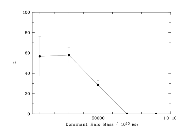
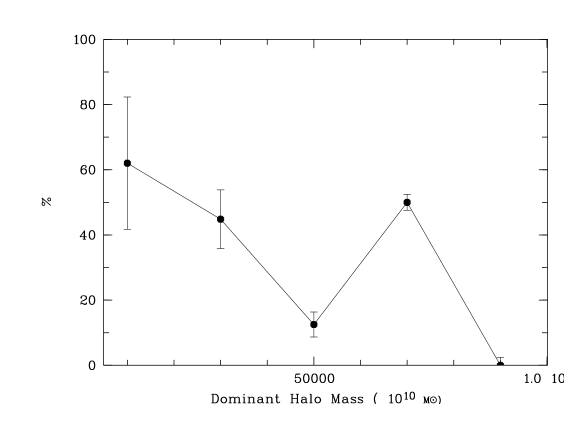
When we investigated the potential effect of the S/N threshold on the substructure level, we did not find any significant tendency for S/N$\geq$3.

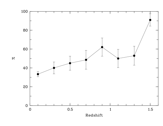
According to the hierarchical structure growth assumed in the Millennium simulation, we could also expect a higher level of substructures with increasing redshift. We do not detect a very clear tendency in the Millenium Wide-like catalog, but Fig. 12 (S/N$\geq$2) seems to show a reverse behaviour for the Millenium Deep-like survey: high redshift $detections$ appear less substructured than nearby ones. However this is at least partially a selection effect explained by the fact that high redshift $detections$ are preferentially low mass structures, less substructured than high mass $detections$ by definition.

Figure 12: Percentage of $detections$ (S/N$\geq$2) with a ratio between the total included mass and the most massive halo mass lower than 3, as a function of redshift for the Deep survey characteristics.

3 Spatial and redshift $detection$ distributions

3.1 $Detection$ counts

Tables LABEL:tab:candD2, LABEL:tab:candD3, LABEL:tab:candD4, LABEL:tab:candW1, LABEL:tab:candW3, and LABEL:tab:candW4, give the $detections$ with their coordinates, redshift, and S/N for the Deep and Wide fields.

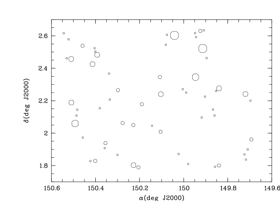
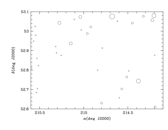
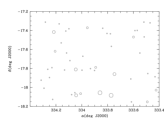
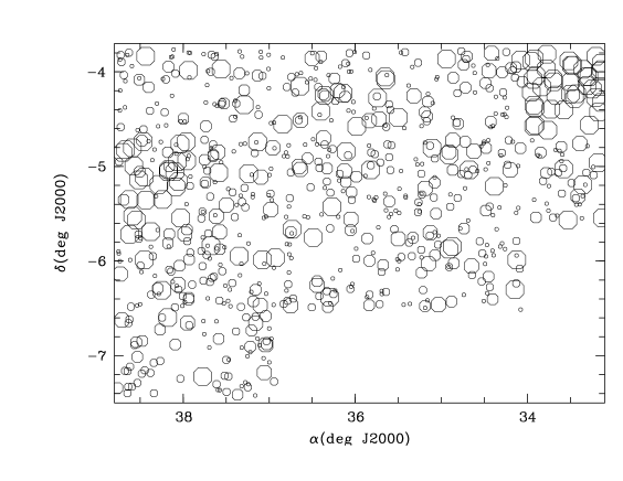
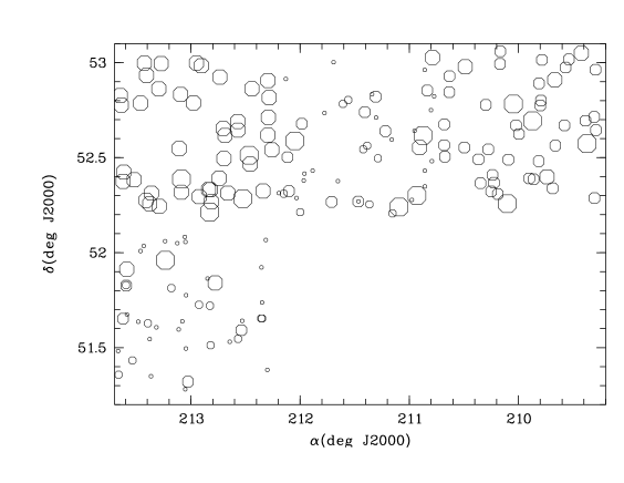
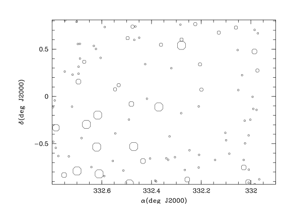
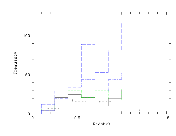
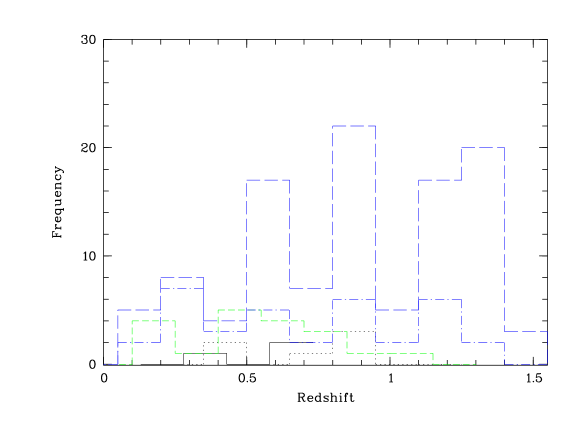
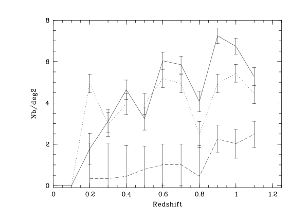
We show in Figs. 13 and  14 the spatial distributions and in Figs. 15,  16, and  17 the redshift distributions of our detections.

We see in Fig. 16 a regular increase in the number of $detections$ as a function of S/N, in good agreement with the expected behaviour of the detection method.

We see in Fig. 17 that the W4 field provides significantly fewer detections (S/N$\geq$2) than W1 and W3. This is not due to a galaxy catalog incompleteness (see Coupon et al. 2009). As seen in Table 1 the numbers of galaxies per deg² for the W1 (250292 gal/deg²), W3 (272147 gal/deg²), and W4 (263685 gal/deg²) fields are similar. Coupon et al. (2009) also find slightly higher uncertainties in the W4 photometric redshift estimates, with a level of catastrophic errors $\sim$35$\%$ higher than in the W1 field. This could have an effect on the cluster detection level. However, this difference in cluster density probably means that the W4 field is intrinsically poor in terms of structures and that this field probably does not include many massive large-scale structures due to cosmic variance.

Figure 13: Spatial distribution of the detected structures in the three searched CFHTLS Deep fields. From top to bottom: D2, D3, and D4. The symbol sizes increase with the S/N of the detection.

Figure 14: Spatial distribution of the detected structures in the three searched CFHTLS Wide fields. From top to bottom: W1, W3, and W4. The symbol sizes increase with the S/N of the detection. Note the different sizes of the three fields, W1 being the largest one. Only W4 covers a full rectangle.

Figure 15: Redshift distribution of the detected structures (S/N$\geq$2) in the searched CFHTLS fields (thin dotted lines: Wide fields, thick continuous line: Deep fields).These histograms are not corrected for detection efficiency.

Figure 16: Redshift distribution of the detected structures in the searched CFHTLS fields as a function of the detection S/N. Continuous black line: S/N=6, dotted black line: S/N=5, dashed green line: S/N=4, dot-dashed blue line: S/N=3, long-dashed blue line: S/N=2. Upper figure: wide fields, lower figure: deep fields. These histograms are not corrected for detection efficiency.

Figure 17: Candidate cluster (S/N$\geq$2) density (per deg²) as a function of redshift. Continuous line: W1 field (computed over 15.73 deg²), dotted line: W3 field (3.24 deg²), dashed line: W4 field (8.87 deg²). Error bars are Poissonian. These curves are not corrected for detection efficiency.

3.2 Angular correlation function

The goal of this subsection is to consider the angular correlation of the distribution of our cluster candidates as a test of consistency of the catalog. If real, $detections$ should not be randomly distributed.

The spatial correlation function of clusters has been known for a long time to behave as a power-law (Bahcall $\&$ Soneira 1983, Nichol et al. 1992):

$$\xi_{cc}(r)=(r/R_{0})^{-\gamma}$$

where the correlation length $R_{0}$ depends on cluster richness and the slope is $\gamma$ $\sim 1.8$. The angular correlation function is then also expected to show a power law behaviour:

$$\omega_{cc}(\theta)=(A_{\omega}(\theta))^{-\delta}$$

with $\delta$=$\gamma$-1.

To estimate the angular correlation of the distribution of our cluster candidates, we limited our sample to the 0.4-0.8 redshift range inside the W1 CFHTLS field in order to both take advantage of the large contiguous coverage of this field and to avoid the redshift range where the W1 field did not provide a high enough detection rate.

The angular two-point correlation function $\omega(\theta)$ represents the excess probability for an object (here a detection) to have a neighbour located at an angular separation $\theta$ with respect to a random distribution of points (Peebles 1980).

We compute the angular correlation using the estimator of Landy & Szalay (1993):

$$\omega(\theta)=\frac{DD(\theta)-2DR(\theta)+RR(\theta)}{RR(\theta)}$$

where DD, RR and DR are respectively the normalised number of data-data, random-random and data-random pairs with an angular separation $\theta$ and $\theta_{i}\leq\theta\leq\theta_{0}+i\times\Delta\theta$. We generate a random catalog of 10000 points with the same geometry and masked as the data. Since the measurement is noisy, we consider several logarithmic binnings and zero points $\theta_{0}$. As a consequence, the measurement at a given angular scale is strongly correlated with the others but the combined measurement gives us at least a qualitative trend, to answer the question of whether or not our sample is randomly spatially distributed.

We do not correct our measurement for the integral constraint due to the finite size of the field (e.g. Cappi & Maurogordato 1995), as the scope of this work is not the clustering analysis itself, but the use of $\omega(\theta)$ as a test of consistency. Our measurement is then a (moderate) underestimate of the real angular correlation function.

We estimate the uncertainty on each data point considering only Poisson errors on the data-data pairs. In the case of the Landy & Szalay estimator, they are given by :

$$\delta\omega=\frac{1+\omega(\theta)}{\sqrt{(}DD(\theta))}$$

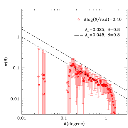
We show in Fig. 18 the combined angular 2-point correlation function in the W1 field for the S/N=3 detection sample. We compare our measurements to two power laws conventionally defined as:

$\omega(\theta)=A_{\omega}(\theta/1^{o})^{-\delta}$

The slope is fixed to $\delta=0.8$ (a reasonable approximation of the true slope) and the amplitude is arbitrarily chosen to guide the eye.

The sample of detections selected with S/N=3 shows a clear signal at large angular scales. A power law with amplitude $A_{\omega}=0.025$ appears to be a good approximation on scales [0.15 – 1] degrees.

At small angular scales, the signal is weaker, and results are not significant, since they are based only on a small number of $detections$, as shown by the large error bars.

This qualitative analysis shows that detections are dominated by structures showing a realistic clustering when compared to other high redshift analyses. Similarly to our results, Papovich (2008) found for example an angular correlation function for his high redshift cluster sample consistent with a power-law fit over the interval [0.03,1.7]deg. The slope of this power law was found to be 1.1$\pm$0.1 in relatively good agreement with our slope of 0.8. Other works such as Bahcall et al. (2003 and references therein) or Brodwin et al. (2007) also show power-law angular correlation functions.

Figure 18: Angular correlation function of our $detections$ in the W1 CFHTLS field for z=[0.4,0.8] for S/N=3. Error bars are Poissonian. The two straight lines are two power laws (see text).

3.3 Tracing the large scale structure of the Universe.

The Millennium simulation, among others, put in evidence the increasing filament constrast (bridges joining massive clusters) with decreasing redshift. This is the well known hierarchical behaviour of the Universe and could ultimately be used as a cosmological test assuming that we are able to trace precisely this filamentary structure as a function of redshift. However, detecting large scale filaments is a very difficult task due to strong superposition effects and to the fact that they are only weak X-ray emitters (see e.g. the Abell 85 filament, Boué et al. 2008). We could in principle consider large scale galaxy surveys such as the CFHTLS combined with photometric redshift computations to try to detect these filaments. However, the galaxies populating these filaments can have very low masses and are therefore likely to be very faint. We must therefore assess the survey depth required to reach such a goal.

Rather than trying to detect individually the filaments present in the CFHTLS survey, we chose a statistical approach based on the Minimal Spanning Tree ($mst$ hereafter) technique. The $mst$ technique is a geometrical construction issued from the graph theory (e.g. Dussert 1988) which allows to characterize quantitatively a distribution of points (e.g. Adami $\&$ Mazure 1999). Very briefly, it is a tree joining all the points of a given set, without any loop and with a minimal length; each point is visited by the tree only once. The main aspect here is the unicity of such a construction. For a given set of points, there is more than one $mst$, but the histogram H of the length of the $mst$ edges is unique. This is fundamental because it is then possible to characterize completely a set of points with H. The details of the procedure and of the normalisations are given in Adami $\&$ Mazure (1999); we took into account the first three momenta (mean, sigma, and skewness) of H to characterize this histogram.

We chose to compute the distance D in the (mean, sigma, skewness) space between a given distribution of points and a uniform distribution for which the mean, sigma, and skewness values are well known (see Adami $\&$ Mazure 1999). The distance D is simply given by:

$$D=\sqrt{\sum_{i=1}^{n}(p_{i}-q_{i})^{2}}$$

with $p_{i}$ and $q_{i}$ being successively the mean, dispersion and skewness of the uniform distribution and of the considered distribution.

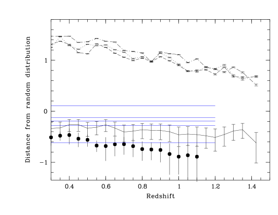
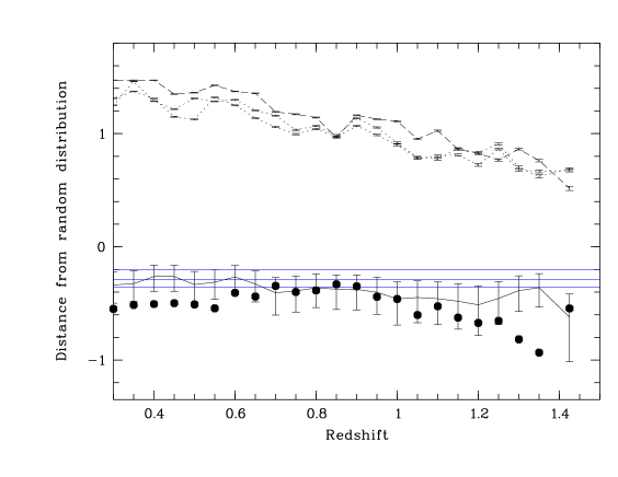
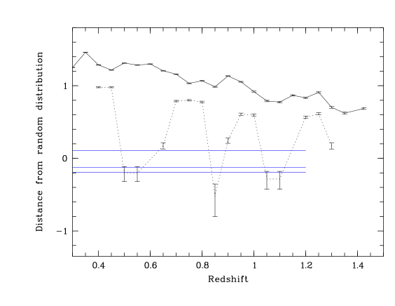
We computed D as a function of redshift in the Millennium simulation. Figs. 19 and  20 show these variations for several halo classes: more massive than 10¹⁰ M_⊙ ($\sim$galaxies), more massive than 3 10¹³ M_⊙ ($\sim$groups of galaxies), more massive than 5 10¹³ M_⊙ ($\sim$major groups of galaxies), and more massive than 10¹⁴ M_⊙ ($\sim$clusters of galaxies). On these figures, a uniform distribution would be a horizontal line at minus infinity.

We first note that our curves all decrease, meaning that the more distant the sample we consider, the closer to a uniform distribution it is. This is not surprising as the main ingredient of the Millennium simulation is a hierarchical gravity dominated Universe.

Second, we plot on these figures the distance D computed with the CFHTLS galaxies in the W1 (Fig. 19) and D2 fields  (Fig.20) assuming the i’=23 and i’=25 magnitude limitations and the computed photometric redshifts. If the CFHTLS fields are good tracers of the large scale structure of the Universe (and if the Millennium simulation assumed the correct cosmology), distances D computed with the CFHTLS data should be included in the Millennium curve for objects more massive than 10¹⁰ M_⊙. We show in Figs. 19 and  20 that the CFHTLS Wide data become different from the expected Millennium behaviour at z$\geq$0.5. This means that the CFHTLS Wide survey is not able to recover properly the filamentary structure of the Universe above z$\sim$0.5. The resulting galaxy distribution (penalized by galaxy detection incompleteness) then becomes too close to a uniform distribution. This also shows that the deep CFHTLS fields are good datasets to achieve such a goal up to z=1.25.

Third, we add on these two figures the distances D computed for our cluster $detections$ and for several values of the detection S/N. We first note that the variation of D with redshift is not significant. We therefore chose to show only the mean value of D over the spanned redshift range (z=[0.1;1.2] for the W1 and z=[0.1;1.5] for the D2). We also find that the higher the S/N (hence the more massive the cluster), the more different from a random distribution the cluster catalogs are. We finally note that the S/N$\geq$4 CFHTLS cluster $detections$ (so with masses greater than 3.3 10¹³ M_⊙) show a different behaviour from Millennium halos more massive than 3 10¹³ M_⊙. The Millennium halos considered are more clustered than the corresponding real clusters (in terms of mass). We now investigate why we have such a difference.

Figure 19: Variation of D as function of redshift. The continuous, dashed, dotted, and dash-dotted lines with error bars are for Millennium halos more massive than 10¹⁰ M_⊙, 3 10¹³ M_⊙, 5 10¹³ M_⊙ , and 10¹⁴ M_⊙. Unconnected filled circles with error bars show the CFHTLS W1 galaxies limited to i’=23. The five horizontal blue lines correspond to the mean D value for clusters detected in the W1 field (from top to bottom: S/N=6, 5, 4, 3, and 2).

Figure 20: Variation of D as function of redshift. The continuous, dashed, dotted, and dash-dotted lines with error bars are for Millennium halos more massive than 10¹⁰ M_⊙, 3 10¹³ M_⊙, 5 10¹³ M_⊙ , and 10¹⁴ M_⊙. Unconnected filled circles with error bars show the CFHTLS D2 galaxies limited to i’=25. The four horizontal blue lines correspond to the mean D value for clusters detected in the D2 field (from top to bottom: S/N=5, 4, 3, and 2). S/N=5 and 4 are overlapping.

Considering low mass Millennium halos implies that highly spatially correlated halos will be included in the $mst$ calculation. This will therefore artificially increase the D value because part of these halos are in fact subhalos of more massive structures. Our $detections$ do not include such objects by definition. A way to not include these highly spatially correlated sub-halos is to select only the less substructured Millennium halos. Therefore, we redid the previous exercise selecting only halos more massive than 3 10¹³ M_⊙ and with a substructure level lower than 20 subhalos included in the main halo. We generated Fig. 21 where we show the D value before and after considering low substructure level halos. We clearly see that removing halos with a high level of substructure makes the Millennium and CFHTLS D values compatible. This suggests that the Millennium simulation may exhibit higher than normal substructure levels in massive clusters.

Figure 21: Variation of D as function of redshift. The continuous and dotted lines with error bars are for Millennium halos more massive than 3 10¹³ M_⊙ with high and low levels of substructures. The three horizontal blue lines are the mean D value for clusters detected in the W1 field (from top to bottom: S/N=6, 5, and 4).

4 Literature assessments of our detections

We computed in previous sections statistical assessments of our detections based on simulations. We now try to compare our detections with literature data, i.e. known clusters in the surveyed areas.

4.1 Internal assessment of our cluster detections.

Among the searched CFHTLS fields, the W1 and D1 fields overlap (see Mazure et al. 2007), allowing us to compare detections based on Deep and Wide CFHTLS data. Wide field data exhibit lower detection rates compared to Deep fields, so we do not expect to recover in the present paper all the D1 detections of Mazure et al. (2007). Assuming the success rates computed in the present paper via the Millennium simulations, we expect to detect 2.7$\pm$1.4 times more clusters in the Deep D1 than in the W1 data (uncertainty from Poisson estimates). Experimentally, we detect 23 clusters in the W1 data out of the 44 detected in the D1 data by Mazure et al. (2007) with exactly the same method. The ratio is 1.9, in agreement with the expectations.

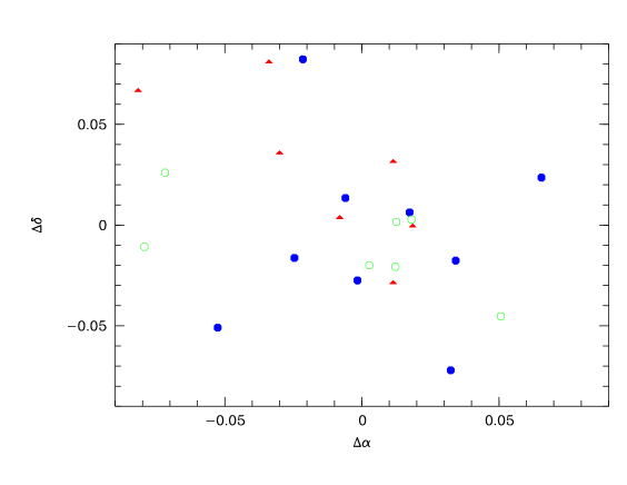
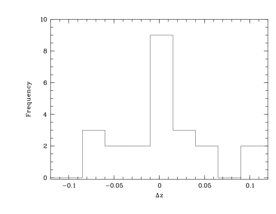
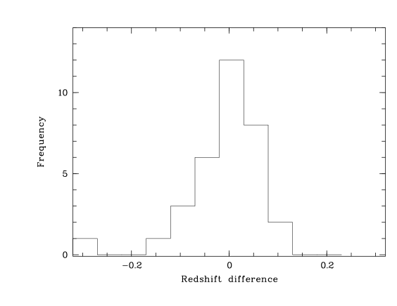
We show in Fig. 22 the position and redshift differences between the present W1 and D1 $detections$ of Mazure et al. (2007). The mean center shift is 0.01$\pm$0.04 deg (0.6 arcmin) and the mean redshift difference is -0.002$\pm$0.05. We also note that there is no significant variation in the center precision as a function of redshift. This demonstrates that we are limited by the pixel size used in the galaxy density map to define a cluster center.

Figure 22: Upper figure: center shifts in deg (blue filled circles: z$\leq$0.5, green open circles: z=[0.5,0.8], red triangles: z$\geq$0.8). Lower figure: histogram of redshift difference between our D1 and W1 $detections$ (S/N$\geq$2).

4.2 External assessment of our cluster detections.

As in Mazure et al. (2007), we compare our $detections$ with the XMM-LSS X-ray clusters published for the W1 field by Pacaud et al. (2007), limiting our comparison to the 15 z$\geq$0.1 clusters of Pacaud et al. (2007) included in the portion of the W1 field we analysed. Ten of our $detections$ are identified with these clusters. The remaining ones (but one) are all affected by masked areas in the optical data and we can reasonably assume that this makes their detection impossible by the present method.

We also compare our $detections$ with the lensing searches made in the CFHTLS areas. Limousin et al. (private communication) discovered a galaxy cluster at z$\sim$0.88 in the CFHTLS D3 field (SL2S2214-1730) based on a strong lensing analysis. This cluster is also detected with our method (D4-7, S/N=2) at z=0.90. A more complete list of group detections in the SL2S survey is given in Limousin et al. (2009). Among the 13 group detections of this paper, a single one (SL2S2140-0532 at z=0.444) is included in our surveyed area (others are outside the area where photometric redshifts were computed) and we detect it at z=0.45 with S/N=6.

We compared our $detections$ with the Gavazzi & Soucail (2007) cluster sample. If we limit our search to clusters with a photometric redshift in their paper (8 clusters), we redetect 7 of these clusters with the present method. The last one is partially located in a masked region in our data and this probably prevents its detection.

We finally compared our $detections$ with the matched filter detections of Olsen et al. (2008). Still limiting the comparison to clusters included in our surveyed area and at z$\geq$0.1, we detect 14 of the 16 Olsen et al. (2008) spectroscopically confirmed clusters.

These high recovery rates therefore put our detection method on a firm ground. We give in Fig. 23 the histograms of the center and redshift differences between our $detections$ and the clusters previously quoted in the literature. The mean center shift is 0.045$\pm$0.03 deg (2.7 arcmin) and the mean redshift difference is -0.01$\pm$0.08.

5 Discussion and Conclusions

We have detected 1200 candidate clusters in the CFHTLS Deep and Wide fields. Statistically, more than 80$\%$ are real structures at z$\leq$1. This is confirmed by internal and external comparisons with literature catalogs.

Table 3: Number and density of $detections$ as a function of S/N.

SExtractor threshold	number of $detections$	density of $detections$
		deg-2
2	535	19.2
3	262	9.4
4	170	6.1
5	98	3.4
6	135	4.8

Table 3 gives the number and density of $detections$ as a function of S/N. Over an effective area of $\sim$28 deg² (see Coupon et al. 2009) this means that we detect 19.2 candidate clusters per deg² for mass $\geq$ 1.0 10¹³M_⊙, 9.4 candidate clusters per deg² for mass $\geq$ 1.3 10¹³M_⊙, 6.1 candidate clusters per deg² for mass $\geq$ 3.3 10¹³M_⊙, 3.4 candidate clusters per deg² for mass $\geq$ 3.5 10¹³M_⊙, and 4.8 candidate clusters per deg² for mass $\geq$ 5.5 10¹³M_⊙. Given the typical uncertainty on detection rates, the two last candidate cluster densities are compatible. We note that these numbers are not corrected for detection efficiency. These numbers are also fully compatible with recent X-ray estimates (e.g. Pacaud et al. 2007) showing detections of 5.8 clusters per deg² for masses greater than 4.1 10¹³M_⊙ (number scaled to our cosmology).

If we compare our results to published optically based cluster catalogs, our survey represents a major step forward (see Table 4). We have one of the deepest and largest cluster catalogs in the CFHTLS area by a factor of $\sim$10 most of the time. We also basically provide the only cluster detections at z$\geq$1 using CFHTLS data. The comparison of our resuls to the well known MaxBCG SDSS catalog (Koester et al. 2007) provides similar numbers in terms of cluster spatial density. The present deep and wide surveys provides more than 13000 and 10500 $detections$ per Gpc³. This is comparable to the 16735 clusters per Gpc³ of Koester et al. (2007), assuming the values of Table 4.

Table 4: Comparison of our cluster detections with public CFHTLS optically based cluster catalogs and with the MaxBCG SDSS catalog.

Authors	Detection method	Covered area	Number of detections	Maximal redshift
		deg2
Present paper Deep	Photometric redshifts	2.5	171	1.5
Present paper Wide	Photometric redshifts	28	1029	1.2
Olsen et al. (2007)	Matched Filter	4	162	1.15
Mazure et al. (2007)	Photometric redshifts	1	44	1.5
Cabanac et al. (2007)	Strong lensing	28	40	1.
Limousin et al. (2009)	Strong lensing	102	13	0.85
Gavazzi $\&$ Soucail (2007)	Weak lensing	4	14	0.55
Bergé et al. (2008)	Weak lensing	4	7	0.5
Koester et al. (2007)	Max BCG	7500	13823	0.3

These results illustrate the power of optical deep and wide field surveys to provide large samples of galaxy clusters. These samples could be used for pure cosmological applications (e.g. based on cluster counts, Romer et al. 2001) or more generally for the study of structures within a broad mass range. In particular, it is remarkable that our deep catalogs are among the first ones to provide numerous group detections at redshifts greater than 1.

In this picture, the perspectives of our work are:

- To perform a more homogeneous comparison with matched filter detections across the Wide fields, and this will be the subject of a future paper. A by-product of this future work will be the center refinement of our candidate clusters.

- To define a more precise optically-based mass estimator, via e.g. the galaxy luminosity functions. This requires however to have performed the previous match.

- To assess more precisely the detection rate for very massive clusters. The Millennium simulation as it is now does not provide a large enough number of very massive structures and this produces too large an uncertainty. This is prohibitive for any serious cosmological application based on cluster counts, since the most massive clusters are the most constraining for cosmology (e.g. Romer et al. 2001) and detection rates for these massive clusters need to be precisely evaluated. This aspect is currently under work and will also be developed in future papers.

- Finally, the spectroscopic confirmation of the z$\geq$1 candidate clusters we have detected would be crucial for cosmology.

The cluster list will be available via the Cencos database at http://cencosw.oamp.fr/ in a near future.

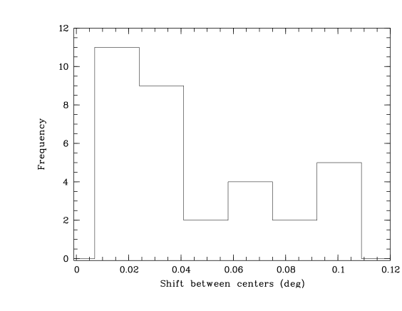
Figure 23: Histograms of the center shifts in degrees (upper figure) and redshift differences (lower figure) between our $detections$ (S/N$\geq$2) and the literature clusters quoted in the text.

Table 5: Candidate clusters detected in the D2 CFHTLS field. The first column is the cluster Id, the second and third columns are the J2000 coordinates given in decimal degrees, the fourth column is the mean redshift, and the fifth column is the SExtractor detection level.

Id	$\alpha$	$\delta$	z	$\sigma_{S}$
D2- 1	149.6931	1.9613	1.20	3.
D2- 2	149.6971	2.2002	0.60	2.
D2- 3	149.7092	1.8994	0.35	2.
D2- 4	149.7174	1.8370	0.63	2.
D2- 5	149.7198	2.2413	1.00	4.
D2- 6	149.7242	1.8689	1.42	2.
D2- 7	149.8395	2.2761	0.40	4.
D2- 8	149.8398	1.8005	0.15	3.
D2- 9	149.8532	2.2603	1.23	2.
D2-10	149.8573	1.7931	0.57	2.
D2-11	149.8596	2.1089	1.35	2.
D2-12	149.8669	2.1456	0.15	2.
D2-13	149.8957	2.4630	0.47	2.
D2-14	149.9035	2.2253	0.80	2.
D2-15	149.9085	2.6340	1.20	2.
D2-16	149.9136	2.5222	0.70	6.
D2-17	149.9180	2.0965	0.68	2.
D2-18	149.9246	2.6301	0.90	3.
D2-19	149.9438	2.5923	0.28	2.
D2-20	149.9464	2.3455	0.95	5.
D2-21	149.9482	2.6171	1.35	2.
D2-22	149.9797	1.8096	0.35	2.
D2-23	149.9884	2.2502	0.45	2.
D2-24	150.0040	2.2709	0.65	2.
D2-25	150.0230	1.8711	1.35	2.
D2-26	150.0417	2.6028	0.68	6.
D2-27	150.0759	2.6058	1.42	2.
D2-28	150.0807	2.5452	0.88	2.
D2-29	150.1032	2.2406	0.75	4.
D2-30	150.1046	2.0085	0.35	3.
D2-31	150.1078	2.3459	0.30	3.
D2-32	150.1434	2.0456	0.75	2.
D2-33	150.1894	2.1784	0.70	3.
D2-34	150.2051	1.7889	0.30	3.
D2-35	150.2275	1.8023	0.45	4.
D2-36	150.2280	2.0504	1.20	3.
D2-37	150.2768	2.0619	1.00	3.
D2-38	150.2985	2.2650	1.10	3.
D2-39	150.3005	1.8659	0.95	2.
D2-40	150.3350	2.2070	0.40	2.
D2-41	150.3383	2.3676	0.70	2.
D2-42	150.3550	1.9385	1.15	3.
D2-43	150.3580	1.9077	1.39	2.
D2-44	150.3807	2.1539	1.10	2.
D2-45	150.3925	2.4827	0.45	4.
D2-46	150.4007	2.5031	1.35	2.
D2-47	150.4010	1.8290	0.90	3.
D2-48	150.4040	2.5237	1.10	2.
D2-49	150.4137	2.4257	0.15	4.
D2-50	150.4237	1.8279	1.00	2.
D2-51	150.4576	1.9729	0.88	2.
D2-52	150.4586	2.5387	0.90	3.
D2-53	150.4826	2.1448	1.42	2.
D2-54	150.4861	2.1086	1.30	2.
D2-55	150.4923	2.0589	0.40	5.
D2-56	150.5093	2.1885	0.80	4.
D2-57	150.5099	2.4570	0.65	4.
D2-58	150.5220	2.5784	1.25	2.
D2-59	150.5306	2.4614	1.15	2.
D2-60	150.5440	2.6161	0.65	2.

Table 6: Same as Table LABEL:tab:candD2 for the D3 CFHTLS field.

Id	$\alpha$	$\delta$	z	$\sigma_{S}$
D3- 1	214.1574	52.4575	0.95	2.
D3- 2	214.1697	52.4380	0.85	2.
D3- 3	214.1903	52.6105	0.60	3.
D3- 4	214.1948	52.8756	1.20	2.
D3- 5	214.2042	53.0803	0.95	5.
D3- 6	214.2207	53.0568	0.60	4.
D3- 7	214.2221	52.3024	0.40	4.
D3- 8	214.2871	52.2871	0.83	2.
D3- 9	214.3238	53.0766	0.30	3.
D3-10	214.3800	52.7434	0.65	5.
D3-11	214.4252	52.4116	0.88	3.
D3-12	214.4484	53.0414	0.65	3.
D3-13	214.4691	52.5612	0.67	4.
D3-14	214.4888	52.7953	1.12	2.
D3-15	214.5119	52.7642	1.35	3.
D3-16	214.5146	52.2788	0.45	3.
D3-17	214.5431	52.5718	1.10	2.
D3-18	214.5678	52.7026	0.15	3.
D3-19	214.5971	52.6576	0.55	2.
D3-20	214.6184	53.0516	1.15	2.
D3-21	214.6637	52.3109	1.15	2.
D3-22	214.6642	52.4382	0.30	2.
D3-23	214.6778	53.0756	0.35	6.
D3-24	214.7280	52.2987	0.28	2.
D3-25	214.7889	52.9131	0.90	2.
D3-26	214.7972	52.6301	0.42	3.
D3-27	214.8425	52.7991	1.30	2.
D3-28	214.8869	52.5894	0.15	4.
D3-29	214.9196	52.5494	0.90	2.
D3-30	214.9200	53.0216	0.78	3.
D3-31	214.9596	52.9875	1.10	3.
D3-32	214.9650	52.5592	0.30	2.
D3-33	214.9922	52.2839	0.90	3.
D3-34	215.0275	52.3052	0.25	3.
D3-35	215.0287	53.0069	1.05	2.
D3-36	215.0379	53.0736	0.18	4.
D3-37	215.0721	52.4805	1.15	2.
D3-38	215.1067	53.0602	0.90	2.
D3-39	215.1351	52.3869	1.00	2.
D3-40	215.1465	52.9367	0.65	4.
D3-41	215.2249	52.3283	0.85	2.
D3-42	215.2558	52.8756	1.40	2.
D3-43	215.2761	53.0428	0.75	4.
D3-44	215.2781	52.2842	1.12	3.
D3-45	215.3089	52.8881	0.60	2.
D3-46	215.3179	52.9212	0.38	2.
D3-47	215.3751	52.3971	0.90	2.
D3-48	215.4052	52.3004	0.83	2.
D3-49	215.4089	52.4817	0.55	2.
D3-50	215.4286	52.4974	0.95	2.
D3-51	215.4299	52.4721	0.15	2.
D3-52	215.4688	52.4534	0.85	3.
D3-53	215.4730	52.2836	0.32	2.
D3-54	215.5046	52.2585	1.15	2.
D3-55	215.5086	52.2857	0.55	2.
D3-56	215.5134	52.8225	0.92	2.
D3-57	215.5195	52.2631	1.30	2.
D3-58	215.5257	52.7045	0.35	2.
D3-59	215.5301	52.8603	0.75	2.
D3-60	215.5363	52.6843	1.00	2.
D3-61	215.5452	52.9787	1.38	2.
D3-62	215.5509	53.0244	1.15	2.
D3-63	215.5692	52.9487	0.70	2.
D3-64	215.5986	52.8094	0.50	3.

Table 7: Same as Table LABEL:tab:candD2 for the D4 CFHTLS field.

Id	$\alpha$	$\delta$	z	$\sigma_{S}$
D4- 1	333.4241	-18.0281	0.50	3.
D4- 2	333.4323	-17.8874	1.15	2.
D4- 3	333.4707	-17.3199	0.65	2.
D4- 4	333.4883	-17.8538	1.27	2.
D4- 5	333.4921	-18.1523	0.60	3.
D4- 6	333.5163	-17.4678	0.90	2.
D4- 7	333.5186	-17.3119	0.15	2.
D4- 8	333.5498	-17.6376	1.40	2.
D4- 9	333.5702	-17.3997	1.38	2.
D4-10	333.5875	-17.4011	1.20	2.
D4-11	333.5992	-17.4693	0.32	3.
D4-12	333.6149	-18.1523	0.85	2.
D4-13	333.6202	-17.9111	1.30	2.
D4-14	333.7466	-17.8600	0.38	4.
D4-15	333.7705	-17.5679	0.85	2.
D4-16	333.7722	-18.0837	0.85	5.
D4-17	333.7782	-17.4350	1.18	2.
D4-18	333.8042	-17.4314	0.73	2.
D4-19	333.8376	-17.3768	1.07	2.
D4-20	333.8589	-18.0563	0.40	5.
D4-21	333.8920	-17.7892	0.42	3.
D4-22	333.9007	-17.8214	1.40	2.
D4-23	333.9324	-17.8020	1.25	2.
D4-24	333.9566	-17.3714	1.30	3.
D4-25	333.9917	-17.6720	0.95	2.
D4-26	333.9981	-17.8181	0.60	2.
D4-27	334.0089	-18.0658	0.30	3.
D4-28	334.0435	-18.0834	0.50	4.
D4-29	334.0461	-17.8109	0.88	4.
D4-30	334.0533	-18.0556	0.85	2.
D4-31	334.0782	-18.0761	0.65	2.
D4-32	334.0915	-17.7177	0.70	2.
D4-33	334.0994	-17.3820	1.40	2.
D4-34	334.1175	-17.6372	1.30	2.
D4-35	334.1234	-17.4064	0.50	2.
D4-36	334.1329	-17.8166	0.53	2.
D4-37	334.1588	-17.5309	0.65	2.
D4-38	334.1748	-17.3305	1.18	2.
D4-39	334.2061	-17.6196	1.05	3.
D4-40	334.2165	-17.4165	0.20	4.
D4-41	334.2252	-18.1266	0.20	2.
D4-42	334.2310	-17.7920	0.83	2.
D4-43	334.2498	-17.8963	0.20	2.
D4-44	334.2632	-17.8097	0.58	2.
D4-45	334.2813	-17.3120	1.25	2.
D4-46	334.2922	-18.0082	0.65	2.
D4-47	334.3143	-17.9242	0.88	2.

Table 8: Same as Table LABEL:tab:candD2 for the W1 CFHTLS field.

Id	$\alpha$	$\delta$	z	$\sigma_{S}$
W1- 1	33.1280	-5.5454	0.32	6.
W1- 2	33.1363	-3.9767	0.57	6.
W1- 3	33.1392	-4.3235	0.75	6.
W1- 4	33.1402	-3.9087	1.07	6.
W1- 5	33.1512	-3.9950	0.90	6.
W1- 6	33.1601	-4.1575	0.60	6.
W1- 7	33.1720	-4.4264	1.00	6.
W1- 8	33.1771	-4.9606	0.55	6.
W1- 9	33.2018	-3.8355	0.42	6.
W1- 10	33.2070	-4.2717	1.10	6.
W1- 11	33.2296	-5.0912	1.05	3.
W1- 12	33.2332	-5.0051	0.70	2.
W1- 13	33.2429	-4.1829	0.95	6.
W1- 14	33.2785	-4.5604	0.93	6.
W1- 15	33.2842	-4.0523	0.47	6.
W1- 16	33.3019	-4.7842	0.63	2.
W1- 17	33.3092	-4.1468	0.65	6.
W1- 18	33.3095	-4.0492	0.82	6.
W1- 19	33.3143	-5.0656	0.80	3.
W1- 20	33.3267	-5.1936	0.80	2.
W1- 21	33.3535	-3.9739	1.10	6.
W1- 22	33.3554	-5.1947	0.43	6.
W1- 23	33.3564	-5.3128	1.10	2.
W1- 24	33.3664	-5.5470	0.75	2.
W1- 25	33.3897	-4.7585	1.00	5.
W1- 26	33.3915	-5.4001	0.60	2.
W1- 27	33.4111	-5.3142	0.72	5.
W1- 28	33.4288	-4.2318	1.05	6.
W1- 29	33.4311	-5.4041	0.47	2.
W1- 30	33.4356	-5.3350	1.00	3.
W1- 31	33.4515	-4.2821	0.63	6.
W1- 32	33.4692	-3.9296	0.97	6.
W1- 33	33.4866	-5.1748	0.82	3.
W1- 34	33.4884	-3.9321	0.45	6.
W1- 35	33.4956	-4.1055	0.65	6.
W1- 36	33.4997	-4.2366	1.10	6.
W1- 37	33.5177	-3.8830	0.55	6.
W1- 38	33.5280	-5.5659	0.45	6.
W1- 39	33.5766	-4.4028	0.43	6.
W1- 40	33.5772	-5.0261	0.50	6.
W1- 41	33.5847	-5.0190	1.05	3.
W1- 42	33.5935	-4.8753	1.05	2.
W1- 43	33.5993	-5.2857	1.10	3.
W1- 44	33.6025	-4.9443	0.28	2.
W1- 45	33.6058	-4.7919	1.00	4.
W1- 46	33.6268	-4.8344	0.70	2.
W1- 47	33.6409	-5.0657	0.82	3.
W1- 48	33.6529	-5.5203	1.00	2.
W1- 49	33.6696	-4.2455	1.00	6.
W1- 50	33.6713	-4.8259	0.85	2.
W1- 51	33.6937	-4.1049	0.43	6.
W1- 52	33.7005	-4.0753	1.10	6.
W1- 53	33.7013	-5.5394	0.45	3.
W1- 54	33.7224	-5.0552	0.98	3.
W1- 55	33.7273	-4.3951	0.68	6.
W1- 56	33.7496	-5.2069	0.50	2.
W1- 57	33.7551	-5.4667	0.70	2.
W1- 58	33.7622	-4.6161	0.34	6.
W1- 59	33.7727	-3.8135	0.81	6.
W1- 60	33.7751	-5.3927	1.10	2.
W1- 61	33.7774	-3.9668	0.55	6.
W1- 62	33.7817	-5.0682	0.80	4.
W1- 63	33.8173	-5.1546	0.70	3.
W1- 64	33.8324	-4.1596	0.95	6.
W1- 65	33.8459	-4.8538	0.60	4.
W1- 66	33.8559	-4.8929	1.10	2.
W1- 67	33.8768	-4.8811	0.85	2.
W1- 68	33.9006	-5.5385	0.28	4.
W1- 69	33.9009	-4.0381	0.40	6.
W1- 70	33.9098	-4.3830	0.40	6.
W1- 71	33.9117	-4.5601	0.70	6.
W1- 72	33.9184	-3.8614	0.57	6.
W1- 73	33.9210	-5.3524	0.85	2.
W1- 74	33.9241	-4.3518	1.00	6.
W1- 75	33.9268	-4.5742	0.88	6.
W1- 76	33.9335	-4.0793	1.07	6.
W1- 77	33.9445	-4.7252	0.63	2.
W1- 78	33.9513	-3.8907	1.10	6.
W1- 79	33.9539	-4.2146	0.34	6.
W1- 80	34.0575	-4.1053	1.10	4.
W1- 81	34.0775	-3.8753	1.10	6.
W1- 82	34.0775	-6.5127	0.40	2.
W1- 83	34.0804	-4.8076	0.55	4.
W1- 84	34.0885	-6.0809	0.77	3.
W1- 85	34.1056	-5.4381	0.30	2.
W1- 86	34.1069	-4.9949	0.85	2.
W1- 87	34.1228	-5.9869	0.47	6.
W1- 88	34.1252	-5.9409	0.82	2.
W1- 89	34.1277	-5.7875	1.07	3.
W1- 90	34.1290	-6.2357	0.90	3.
W1- 91	34.1293	-5.4889	0.68	2.
W1- 92	34.1338	-3.9501	0.40	4.
W1- 93	34.1431	-4.0622	0.85	3.
W1- 94	34.1454	-6.3026	0.50	6.
W1- 95	34.1692	-4.7383	0.30	2.
W1- 96	34.1707	-3.9844	0.65	3.
W1- 97	34.1882	-3.9599	0.95	4.
W1- 98	34.1994	-5.0378	0.40	5.
W1- 99	34.2174	-4.7230	0.15	3.
W1-100	34.2296	-4.9823	0.98	3.
W1-101	34.2345	-4.3798	1.02	2.
W1-102	34.2421	-4.4784	0.77	2.
W1-103	34.2445	-3.7907	0.55	3.
W1-104	34.2548	-5.1998	1.00	2.
W1-105	34.2595	-5.8731	0.40	2.
W1-106	34.2640	-4.2716	1.10	2.
W1-107	34.2661	-4.4491	1.10	2.
W1-108	34.2814	-4.2169	0.85	3.
W1-109	34.2882	-4.4518	0.90	2.
W1-110	34.2928	-4.0056	0.70	4.
W1-111	34.2933	-5.8127	0.50	2.
W1-112	34.2966	-4.8562	1.10	3.
W1-113	34.3064	-4.8831	0.63	2.
W1-114	34.3158	-5.8461	1.10	2.
W1-115	34.3238	-5.4346	0.60	2.
W1-116	34.3481	-3.8583	0.15	2.
W1-117	34.3571	-5.6630	0.45	2.
W1-118	34.3662	-4.2637	0.45	2.
W1-119	34.3676	-4.4420	0.95	2.
W1-120	34.3828	-5.2103	0.65	6.
W1-121	34.3921	-5.9389	0.50	2.
W1-122	34.4001	-5.5150	0.85	2.
W1-123	34.4003	-4.5730	0.25	2.
W1-124	34.4033	-6.4039	1.05	4.
W1-125	34.4056	-5.8900	0.85	2.
W1-126	34.4161	-3.8044	0.25	5.
W1-127	34.4249	-4.5280	0.50	4.
W1-128	34.4251	-4.5848	0.68	2.
W1-129	34.4366	-6.2746	0.98	3.
W1-130	34.4392	-4.1727	0.38	3.
W1-131	34.4398	-5.4236	1.00	3.
W1-132	34.4467	-3.9897	0.68	5.
W1-133	34.4510	-6.1641	0.55	4.
W1-134	34.4528	-4.9648	1.05	2.
W1-135	34.4541	-4.7226	0.90	2.
W1-136	34.4594	-3.9263	0.80	2.
W1-137	34.4664	-6.3393	0.88	2.
W1-138	34.4694	-5.8299	0.80	2.
W1-139	34.4803	-4.8054	0.50	4.
W1-140	34.4804	-5.9505	0.65	2.
W1-141	34.4831	-5.4664	0.80	4.
W1-142	34.4850	-5.0315	1.00	2.
W1-143	34.4872	-4.1193	1.05	4.
W1-144	34.4914	-6.0300	0.98	2.
W1-145	34.5029	-4.7390	1.10	2.
W1-146	34.5068	-6.4222	0.68	2.
W1-147	34.5091	-4.7563	0.75	2.
W1-148	34.5226	-5.9188	0.40	3.
W1-149	34.5311	-6.2150	1.05	3.
W1-150	34.5370	-4.7876	0.33	2.
W1-151	34.5536	-5.7914	0.85	3.
W1-152	34.5806	-5.0485	1.10	2.
W1-153	34.6086	-4.2178	0.15	2.
W1-154	34.6115	-4.0119	0.33	2.
W1-155	34.6207	-4.8404	1.10	5.
W1-156	34.6284	-3.9344	0.60	2.
W1-157	34.6331	-5.0330	0.80	3.
W1-158	34.6435	-6.1477	0.70	3.
W1-159	34.6498	-6.0529	1.05	5.
W1-160	34.6756	-5.0365	0.50	6.
W1-161	34.6875	-5.0908	1.10	3.
W1-162	34.6880	-5.5716	0.70	2.
W1-163	34.7034	-3.8378	0.95	4.
W1-164	34.7065	-5.0305	0.93	2.
W1-165	34.7116	-3.8647	0.80	3.
W1-166	34.7188	-4.1670	0.50	4.
W1-167	34.7226	-4.7386	0.82	4.
W1-168	34.7236	-5.2310	0.33	2.
W1-169	34.7367	-5.6567	0.75	4.
W1-170	34.7384	-6.3570	0.95	2.
W1-171	34.7411	-3.9266	1.05	4.
W1-172	34.7668	-3.7838	0.90	3.
W1-173	34.7687	-5.0803	0.75	3.
W1-174	34.7800	-5.6568	0.85	2.
W1-175	34.8040	-4.5489	0.75	4.
W1-176	34.8107	-5.3332	0.85	3.
W1-177	34.8133	-4.2251	0.82	3.
W1-178	34.8196	-4.5380	0.95	3.
W1-179	34.8550	-6.0232	1.00	4.
W1-180	34.8619	-4.0631	0.80	4.
W1-181	34.8646	-4.4844	0.15	2.
W1-182	34.8660	-4.7243	0.85	5.
W1-183	34.8686	-5.0375	1.10	4.
W1-184	34.8719	-5.8459	0.65	6.
W1-185	34.8812	-6.4285	0.65	4.
W1-186	34.8950	-5.2962	0.60	2.
W1-187	34.8959	-5.4255	0.45	3.
W1-188	34.9089	-6.0626	0.80	3.
W1-189	34.9092	-4.8757	0.33	6.
W1-190	34.9107	-4.8460	0.85	5.
W1-191	34.9115	-6.0623	0.50	2.
W1-192	34.9129	-5.8745	0.36	6.
W1-193	34.9401	-3.8648	0.73	6.
W1-194	35.0326	-5.7321	0.70	2.
W1-195	35.0340	-6.4613	0.65	5.
W1-196	35.0386	-5.8267	1.05	3.
W1-197	35.0476	-4.0556	1.02	2.
W1-198	35.0557	-4.0770	0.68	2.
W1-199	35.0612	-5.4980	0.50	4.
W1-200	35.0729	-5.9385	0.80	4.
W1-201	35.0750	-4.9162	0.60	3.
W1-202	35.0760	-5.6944	1.10	2.
W1-203	35.0766	-5.1154	1.10	2.
W1-204	35.0780	-5.1710	0.73	4.
W1-205	35.0870	-5.3282	0.55	3.
W1-206	35.1000	-4.3303	1.00	2.
W1-207	35.1080	-4.8051	1.00	6.
W1-208	35.1285	-5.7007	0.40	5.
W1-209	35.1311	-4.7804	0.43	3.
W1-210	35.1337	-5.7307	0.88	3.
W1-211	35.1475	-6.0285	0.35	5.
W1-212	35.1537	-4.2327	0.52	2.
W1-213	35.1560	-4.3150	0.90	4.
W1-214	35.1602	-6.4158	1.10	2.
W1-215	35.1650	-4.4717	1.00	4.
W1-216	35.1693	-4.5216	0.88	3.
W1-217	35.1874	-6.4949	0.85	2.
W1-218	35.1877	-5.2307	1.10	5.
W1-219	35.1895	-6.4755	0.60	4.
W1-220	35.1897	-4.7486	0.70	2.
W1-221	35.1937	-4.4259	0.80	4.
W1-222	35.2123	-6.3068	0.70	3.
W1-223	35.2225	-4.9736	0.65	2.
W1-224	35.2259	-5.2966	1.05	3.
W1-225	35.2293	-5.9614	1.02	2.
W1-226	35.2295	-6.1228	0.90	4.
W1-227	35.2300	-4.5738	0.80	2.
W1-228	35.2308	-5.2894	0.50	2.
W1-229	35.2320	-5.0772	1.00	3.
W1-230	35.2337	-5.8808	0.75	3.
W1-231	35.2542	-5.4759	1.10	2.
W1-232	35.2549	-5.3996	0.52	2.
W1-233	35.2646	-5.3783	0.95	3.
W1-234	35.2697	-3.9034	0.35	3.
W1-235	35.2709	-5.4826	0.25	3.
W1-236	35.2783	-4.9794	1.05	2.
W1-237	35.2960	-4.9247	0.40	2.
W1-238	35.3186	-4.2550	0.90	5.
W1-239	35.3271	-5.7538	1.00	2.
W1-240	35.3300	-5.7545	0.85	4.
W1-241	35.3371	-3.9482	1.10	2.
W1-242	35.3422	-5.9477	0.45	3.
W1-243	35.3644	-6.4523	1.05	2.
W1-244	35.3740	-5.8053	0.60	3.
W1-245	35.3797	-4.1451	0.33	2.
W1-246	35.4139	-5.3278	0.88	2.
W1-247	35.4143	-5.3104	0.75	2.
W1-248	35.4219	-3.7920	0.47	3.
W1-249	35.4300	-4.5950	0.73	2.
W1-250	35.4375	-6.4620	0.95	2.
W1-251	35.4648	-5.9564	0.73	3.
W1-252	35.4681	-5.0476	0.75	2.
W1-253	35.4687	-3.7963	0.75	2.
W1-254	35.4865	-5.2363	1.02	2.
W1-255	35.4894	-6.0005	1.10	2.
W1-256	35.4895	-5.4922	0.82	2.
W1-257	35.5001	-4.4844	0.28	6.
W1-258	35.5009	-5.7646	0.80	5.
W1-259	35.5090	-6.0885	0.55	2.
W1-260	35.5103	-5.9816	0.95	2.
W1-261	35.5281	-5.4679	1.00	2.
W1-262	35.5458	-5.6629	0.45	3.
W1-263	35.5811	-4.7759	0.50	3.
W1-264	35.5837	-5.5022	0.40	2.
W1-265	35.5918	-4.4020	0.45	3.
W1-266	35.5918	-5.0385	0.95	3.
W1-267	35.6043	-5.3711	0.45	4.
W1-268	35.6060	-4.9028	1.10	3.
W1-269	35.6078	-5.5335	0.75	2.
W1-270	35.6082	-4.3431	0.82	3.
W1-271	35.6257	-4.7680	0.85	3.
W1-272	35.6329	-4.0344	0.90	2.
W1-273	35.6407	-4.5815	0.63	3.
W1-274	35.6422	-5.4630	0.30	2.
W1-275	35.6430	-6.3261	0.73	3.
W1-276	35.6454	-4.0824	1.02	6.
W1-277	35.6499	-4.5687	0.93	2.
W1-278	35.6526	-4.0547	0.70	6.
W1-279	35.6532	-5.2879	1.10	2.
W1-280	35.6774	-6.0418	0.30	4.
W1-281	35.6917	-6.3477	0.47	2.
W1-282	35.6929	-6.3159	1.07	2.
W1-283	35.6944	-6.1144	0.73	3.
W1-284	35.7094	-4.9587	0.80	3.
W1-285	35.7173	-6.4566	1.00	3.
W1-286	35.7229	-4.4986	0.80	5.
W1-287	35.7318	-5.6438	0.25	2.
W1-288	35.7403	-4.2774	0.43	6.
W1-289	35.7485	-4.2589	0.65	3.
W1-290	35.7580	-5.3276	0.88	2.
W1-291	35.7740	-4.8702	1.10	3.
W1-292	35.7763	-5.3629	0.75	2.
W1-293	35.7800	-4.3884	0.20	2.
W1-294	35.7840	-5.3481	0.50	2.
W1-295	35.7935	-5.9133	1.00	2.
W1-296	35.8145	-4.8518	0.65	3.
W1-297	35.8192	-4.9895	0.55	3.
W1-298	35.8232	-5.0362	0.40	6.
W1-299	35.8246	-3.9794	1.10	2.
W1-300	35.8333	-6.3542	0.40	3.
W1-301	35.8352	-5.9978	1.10	4.
W1-302	35.8356	-4.5168	1.00	5.
W1-303	35.8390	-6.4668	0.50	4.
W1-304	35.8396	-4.7796	0.30	2.
W1-305	35.8422	-5.3229	0.38	2.
W1-306	35.8610	-5.7614	0.33	4.
W1-307	35.8629	-6.3806	0.70	2.
W1-308	35.8693	-4.4874	0.47	2.
W1-309	35.8722	-3.8268	1.02	3.
W1-310	35.8827	-5.1001	0.90	2.
W1-311	35.9826	-4.5789	0.47	6.
W1-312	35.9881	-5.1078	0.90	4.
W1-313	35.9896	-5.8691	0.47	2.
W1-314	35.9901	-5.9752	1.07	3.
W1-315	36.0069	-3.7898	0.88	2.
W1-316	36.0201	-4.4246	0.82	2.
W1-317	36.0225	-4.3179	0.98	2.
W1-318	36.0316	-5.6827	1.00	2.
W1-319	36.0343	-6.2426	0.80	2.
W1-320	36.0407	-5.3537	0.80	3.
W1-321	36.0434	-5.2714	0.55	4.
W1-322	36.0474	-3.9963	0.48	2.
W1-323	36.0486	-6.2716	0.33	2.
W1-324	36.0510	-5.5572	0.50	5.
W1-325	36.0542	-5.6732	0.80	4.
W1-326	36.0565	-6.2946	0.60	3.
W1-327	36.0673	-3.8023	0.45	3.
W1-328	36.0739	-3.9983	0.30	2.
W1-329	36.0784	-4.4098	0.15	2.
W1-330	36.0812	-3.9137	0.95	2.
W1-331	36.0837	-4.8820	1.05	3.
W1-332	36.1075	-4.8427	0.55	6.
W1-333	36.1095	-5.1645	0.95	4.
W1-334	36.1138	-3.9077	1.05	3.
W1-335	36.1172	-4.2633	1.00	4.
W1-336	36.1259	-5.0493	0.52	5.
W1-337	36.1381	-4.1615	1.10	2.
W1-338	36.1412	-5.2609	1.10	2.
W1-339	36.1424	-4.2269	0.33	6.
W1-340	36.1737	-6.0957	0.38	2.
W1-341	36.1773	-3.9457	1.10	2.
W1-342	36.1818	-5.0775	0.77	3.
W1-343	36.1870	-5.1485	1.05	2.
W1-344	36.1979	-5.5325	0.80	2.
W1-345	36.2062	-4.1967	0.70	5.
W1-346	36.2307	-4.3084	0.95	3.
W1-347	36.2335	-6.3121	1.10	2.
W1-348	36.2422	-4.0705	0.80	4.
W1-349	36.2532	-6.3501	0.45	3.
W1-350	36.2610	-6.1840	0.73	2.
W1-351	36.2644	-4.8157	1.10	3.
W1-352	36.2713	-5.4248	0.47	6.
W1-353	36.2787	-4.5127	0.70	2.
W1-354	36.2890	-5.2774	0.70	3.
W1-355	36.2919	-6.4445	0.60	2.
W1-356	36.2921	-5.6544	0.40	3.
W1-357	36.2994	-6.3815	0.30	6.
W1-358	36.3016	-4.8240	0.40	2.
W1-359	36.3103	-4.0356	1.05	2.
W1-360	36.3162	-4.8910	0.77	2.
W1-361	36.3183	-6.4858	0.75	4.
W1-362	36.3283	-5.0214	0.40	4.
W1-363	36.3297	-5.1591	0.88	3.
W1-364	36.3305	-6.3173	0.95	3.
W1-365	36.3500	-4.2550	0.50	4.
W1-366	36.3535	-5.2266	0.45	2.
W1-367	36.3558	-4.7683	0.55	3.
W1-368	36.3615	-4.2487	0.15	6.
W1-369	36.3692	-4.7006	0.28	5.
W1-370	36.3694	-4.2367	1.02	4.
W1-371	36.3913	-5.5069	0.55	2.
W1-372	36.3963	-3.8370	0.80	4.
W1-373	36.4006	-4.4175	0.88	6.
W1-374	36.4008	-3.8957	1.10	2.
W1-375	36.4138	-4.4545	0.68	2.
W1-376	36.4164	-5.0157	0.60	3.
W1-377	36.4187	-6.3715	0.85	3.
W1-378	36.4288	-4.9489	0.98	3.
W1-379	36.4308	-4.1596	0.75	3.
W1-380	36.4428	-6.2565	0.60	5.
W1-381	36.4432	-6.2121	0.85	4.
W1-382	36.4448	-4.7661	1.10	2.
W1-383	36.4566	-3.9614	0.85	2.
W1-384	36.4634	-4.0848	0.70	2.
W1-385	36.4881	-5.7503	0.64	6.
W1-386	36.4898	-4.7130	0.63	2.
W1-387	36.4999	-3.8040	0.70	2.
W1-388	36.5020	-3.8570	0.40	5.
W1-389	36.5055	-6.4890	0.60	3.
W1-390	36.5179	-4.0710	0.57	2.
W1-391	36.5198	-5.2201	0.50	3.
W1-392	36.5490	-5.5366	0.80	2.
W1-393	36.5549	-4.9141	1.05	4.
W1-394	36.5618	-4.1103	0.93	2.
W1-395	36.5823	-4.7695	0.85	2.
W1-396	36.5908	-5.5278	1.00	2.
W1-397	36.6316	-4.0126	0.65	2.
W1-398	36.6350	-4.5123	0.30	5.
W1-399	36.6389	-5.0308	0.85	5.
W1-400	36.6404	-4.4789	0.93	2.
W1-401	36.6430	-4.1512	0.30	6.
W1-402	36.6530	-4.9993	0.52	5.
W1-403	36.6560	-4.5112	0.68	3.
W1-404	36.6799	-4.0261	1.10	2.
W1-405	36.6977	-4.2198	0.75	3.
W1-406	36.7212	-6.3970	1.10	3.
W1-407	36.7348	-5.6644	0.35	6.
W1-408	36.7383	-5.7071	1.00	2.
W1-409	36.7424	-4.0545	0.75	3.
W1-410	36.7433	-5.9685	0.80	2.
W1-411	36.7483	-5.6945	0.80	4.
W1-412	36.7492	-5.0628	0.20	3.
W1-413	36.7518	-6.4715	0.68	5.
W1-414	36.7618	-5.3350	0.51	3.
W1-415	36.7627	-5.8241	0.60	2.
W1-416	36.7673	-5.9293	0.95	2.
W1-417	36.7703	-5.4247	1.10	2.
W1-418	36.7705	-6.1208	1.10	2.
W1-419	36.7736	-4.7760	0.95	2.
W1-420	36.7797	-6.2453	1.00	3.
W1-421	36.7860	-4.8942	1.10	2.
W1-422	36.7889	-6.4198	1.00	3.
W1-423	36.7953	-4.1606	0.88	3.
W1-424	36.7957	-5.8209	1.10	2.
W1-425	36.7998	-6.3121	0.57	2.
W1-426	36.8038	-5.5333	0.55	2.
W1-427	36.8041	-4.8538	0.70	2.
W1-428	36.8291	-4.8915	0.28	2.
W1-429	36.8311	-6.4530	0.40	3.
W1-430	36.8407	-3.8492	0.95	2.
W1-431	36.8432	-4.5535	0.30	6.
W1-432	36.9290	-5.9664	0.25	6.
W1-433	36.9389	-4.8076	0.45	2.
W1-434	36.9435	-7.2736	0.30	3.
W1-435	36.9439	-4.5376	0.65	2.
W1-436	36.9456	-6.0701	1.00	2.
W1-437	36.9490	-6.4629	0.95	2.
W1-438	36.9588	-4.8037	1.00	5.
W1-439	36.9691	-5.3557	0.77	2.
W1-440	36.9744	-6.8204	1.10	2.
W1-441	36.9786	-4.5418	1.05	2.
W1-442	36.9788	-5.0244	1.10	2.
W1-443	36.9812	-5.4562	0.50	5.
W1-444	36.9848	-5.2873	0.45	3.
W1-445	36.9959	-5.0908	0.43	2.
W1-446	36.9992	-7.0704	0.20	2.
W1-447	36.9999	-6.7123	0.75	2.
W1-448	37.0041	-4.1735	0.57	2.
W1-449	37.0055	-5.3031	0.33	2.
W1-450	37.0064	-3.8201	1.10	2.
W1-451	37.0090	-3.9693	0.85	2.
W1-452	37.0303	-6.8807	0.80	4.
W1-453	37.0306	-6.8460	0.90	3.
W1-454	37.0349	-6.3444	1.02	2.
W1-455	37.0363	-5.5297	0.90	2.
W1-456	37.0397	-6.5815	0.75	4.
W1-457	37.0405	-6.8843	0.50	5.
W1-458	37.0571	-6.0283	0.50	2.
W1-459	37.0575	-7.1788	0.35	5.
W1-460	37.0637	-5.5436	0.73	2.
W1-461	37.0657	-7.0267	0.93	2.
W1-462	37.0774	-4.0435	1.10	3.
W1-463	37.0781	-5.9869	0.75	6.
W1-464	37.0941	-3.8495	0.25	2.
W1-465	37.0971	-5.1123	0.80	5.
W1-466	37.0986	-3.7886	1.00	2.
W1-467	37.1050	-6.4686	0.75	5.
W1-468	37.1124	-6.8893	1.05	2.
W1-469	37.1158	-6.2391	0.43	2.
W1-470	37.1245	-4.4530	0.82	3.
W1-471	37.1307	-4.3739	1.10	2.
W1-472	37.1355	-4.7416	0.63	6.
W1-473	37.1371	-4.0400	0.35	4.
W1-474	37.1374	-6.8180	0.82	2.
W1-475	37.1504	-4.7448	0.80	2.
W1-476	37.1570	-6.6569	0.48	5.
W1-477	37.1587	-6.3042	0.68	4.
W1-478	37.1595	-6.5878	1.10	3.
W1-479	37.1622	-7.4206	0.45	2.
W1-480	37.1678	-4.8583	1.00	3.
W1-481	37.1849	-6.4266	0.45	4.
W1-482	37.1898	-5.2929	0.50	2.
W1-483	37.1926	-5.3230	1.00	2.
W1-484	37.2048	-5.0872	0.98	2.
W1-485	37.2060	-6.7342	1.10	4.
W1-486	37.2082	-6.3262	0.90	2.
W1-487	37.2203	-6.9630	0.68	2.
W1-488	37.2206	-6.9052	0.95	4.
W1-489	37.2395	-5.0742	0.25	6.
W1-490	37.2412	-5.8146	0.95	2.
W1-491	37.2428	-7.3016	0.15	2.
W1-492	37.2486	-7.3331	0.35	3.
W1-493	37.2528	-7.0063	0.22	2.
W1-494	37.2585	-4.0152	0.60	2.
W1-495	37.2671	-6.5949	0.40	3.
W1-496	37.2769	-7.2820	0.85	2.
W1-497	37.2791	-5.4318	1.10	3.
W1-498	37.2821	-4.7591	0.55	2.
W1-499	37.2880	-5.2261	0.65	3.
W1-500	37.2908	-4.3480	0.40	6.
W1-501	37.2918	-4.1940	0.83	4.
W1-502	37.3144	-3.8395	0.30	2.
W1-503	37.3167	-5.3743	0.37	3.
W1-504	37.3200	-6.9147	1.10	2.
W1-505	37.3209	-7.3220	1.07	2.
W1-506	37.3233	-6.0295	0.98	2.
W1-507	37.3284	-6.4839	0.65	3.
W1-508	37.3298	-4.7643	0.70	2.
W1-509	37.3307	-5.3091	0.80	2.
W1-510	37.3394	-6.1506	0.60	2.
W1-511	37.3428	-5.7267	1.07	2.
W1-512	37.3441	-3.7844	0.75	2.
W1-513	37.3473	-4.0156	0.45	4.
W1-514	37.3495	-5.9472	0.32	6.
W1-515	37.3681	-7.4121	0.47	4.
W1-516	37.3778	-5.4065	0.70	2.
W1-517	37.3826	-4.3358	0.70	3.
W1-518	37.3854	-6.7435	1.10	3.
W1-519	37.3931	-4.4746	1.10	2.
W1-520	37.3955	-4.3060	0.50	2.
W1-521	37.4000	-5.5353	0.70	3.
W1-522	37.4120	-4.8414	1.10	2.
W1-523	37.4211	-4.4953	0.95	3.
W1-524	37.4271	-5.2728	0.70	3.
W1-525	37.4299	-6.2329	0.85	3.
W1-526	37.4393	-4.0658	0.30	2.
W1-527	37.4506	-6.4770	0.73	2.
W1-528	37.4571	-6.3016	0.47	2.
W1-529	37.4698	-7.0419	0.70	2.
W1-530	37.4738	-7.2186	0.70	3.
W1-531	37.4762	-5.2388	0.43	2.
W1-532	37.4782	-6.4208	0.38	2.
W1-533	37.4958	-7.3830	0.30	3.
W1-534	37.4973	-5.4074	0.45	5.
W1-535	37.4998	-7.0444	0.85	3.
W1-536	37.5095	-6.2601	1.05	2.
W1-537	37.5182	-7.2122	1.00	3.
W1-538	37.5192	-5.8551	0.60	2.
W1-539	37.5257	-4.3337	0.45	4.
W1-540	37.5270	-6.4470	0.88	2.
W1-541	37.5454	-6.1078	0.45	3.
W1-542	37.5456	-4.3247	1.10	3.
W1-543	37.5535	-4.3422	0.77	3.
W1-544	37.5581	-4.9568	0.80	2.
W1-545	37.5604	-3.9713	0.68	6.
W1-546	37.5680	-6.0390	1.00	2.
W1-547	37.5749	-5.8747	0.35	4.
W1-548	37.5753	-7.3643	0.95	2.
W1-549	37.5777	-5.6931	0.57	5.
W1-550	37.5790	-6.4178	1.05	3.
W1-551	37.5875	-5.0661	1.10	6.
W1-552	37.5878	-6.8218	0.81	4.
W1-553	37.5955	-7.3624	0.73	2.
W1-554	37.5962	-4.8481	0.95	5.
W1-555	37.6070	-4.3592	1.05	2.
W1-556	37.6077	-5.8687	0.90	2.
W1-557	37.6108	-3.8121	0.82	2.
W1-558	37.6121	-7.3013	0.35	3.
W1-559	37.6136	-6.6373	0.98	2.
W1-560	37.6152	-5.5268	1.00	5.
W1-561	37.6281	-5.5159	0.60	2.
W1-562	37.6308	-5.1656	0.80	2.
W1-563	37.6337	-4.3422	0.90	2.
W1-564	37.6353	-3.8408	1.10	3.
W1-565	37.6434	-6.1662	0.85	3.
W1-566	37.6500	-4.8782	0.80	4.
W1-567	37.6508	-4.8904	1.05	4.
W1-568	37.6518	-4.7668	0.65	3.
W1-569	37.6644	-6.1780	0.43	3.
W1-570	37.6697	-3.8202	0.60	3.
W1-571	37.6766	-5.8387	1.10	6.
W1-572	37.6775	-4.8071	0.90	2.
W1-573	37.6788	-3.9993	0.55	3.
W1-574	37.6863	-5.3178	0.95	3.
W1-575	37.6896	-6.2216	0.65	3.
W1-576	37.6916	-5.9735	0.45	2.
W1-577	37.6953	-6.9133	1.10	2.
W1-578	37.7087	-5.7084	0.80	3.
W1-579	37.7128	-3.9917	0.30	2.
W1-580	37.7138	-6.3949	1.05	2.
W1-581	37.7150	-5.8384	0.95	2.
W1-582	37.7200	-5.0448	0.63	3.
W1-583	37.7220	-4.1406	0.77	2.
W1-584	37.7281	-5.9349	0.85	3.
W1-585	37.7355	-4.5741	0.65	4.
W1-586	37.7368	-4.3238	0.73	2.
W1-587	37.7412	-5.1695	0.50	4.
W1-588	37.7492	-4.9297	0.95	4.
W1-589	37.7497	-5.1827	1.05	3.
W1-590	37.7515	-5.0040	1.05	2.
W1-591	37.7527	-4.7186	1.05	3.
W1-592	37.7551	-6.7718	0.85	2.
W1-593	37.7624	-3.8127	1.05	2.
W1-594	37.7648	-6.2066	0.90	3.
W1-595	37.7651	-6.6340	1.10	2.
W1-596	37.7710	-5.4789	0.85	2.
W1-597	37.7726	-5.7504	0.65	2.
W1-598	37.7732	-7.2195	0.28	6.
W1-599	37.7751	-6.0533	0.70	3.
W1-600	37.7761	-5.4775	1.00	3.
W1-601	37.7876	-5.8943	0.55	3.
W1-602	37.7879	-5.5489	0.40	3.
W1-603	37.8955	-6.2486	0.65	3.
W1-604	37.9157	-5.1068	0.70	2.
W1-605	37.9175	-5.9106	0.85	3.
W1-606	37.9196	-3.8003	0.93	2.
W1-607	37.9213	-5.2061	0.65	3.
W1-608	37.9275	-4.0593	1.00	2.
W1-609	37.9302	-6.6784	0.85	3.
W1-610	37.9315	-5.9839	0.70	4.
W1-611	37.9338	-6.3877	0.75	4.
W1-612	37.9364	-4.8895	0.75	2.
W1-613	37.9369	-6.4057	1.05	4.
W1-614	37.9372	-3.7971	0.60	2.
W1-615	37.9372	-3.9857	1.10	6.
W1-616	37.9492	-4.9230	0.63	2.
W1-617	37.9501	-6.6544	0.30	5.
W1-618	37.9522	-5.7906	0.73	3.
W1-619	37.9564	-5.6668	0.90	4.
W1-620	37.9598	-4.9418	0.98	6.
W1-621	37.9611	-5.3980	0.50	2.
W1-622	37.9642	-4.7386	1.05	6.
W1-623	37.9796	-6.4334	0.25	2.
W1-624	37.9799	-5.7154	0.40	5.
W1-625	37.9823	-4.5252	0.45	2.
W1-626	37.9979	-4.4967	0.70	4.
W1-627	38.0054	-6.3694	0.50	3.
W1-628	38.0096	-6.4742	0.85	2.
W1-629	38.0283	-5.5459	0.60	6.
W1-630	38.0290	-4.5217	0.93	2.
W1-631	38.0325	-7.2426	1.10	3.
W1-632	38.0373	-4.7646	0.98	6.
W1-633	38.0426	-6.0490	0.40	4.
W1-634	38.0533	-5.1593	0.33	6.
W1-635	38.0542	-6.3023	0.90	3.
W1-636	38.0596	-6.2475	0.30	5.
W1-637	38.0676	-4.9485	0.85	6.
W1-638	38.0754	-6.2613	1.05	2.
W1-639	38.0805	-4.8644	0.50	2.
W1-640	38.0816	-4.7717	0.55	2.
W1-641	38.0844	-5.2144	0.95	6.
W1-642	38.0893	-4.0189	0.17	3.
W1-643	38.0919	-6.8821	0.68	4.
W1-644	38.0960	-6.4897	0.65	3.
W1-645	38.0985	-5.0565	0.80	6.
W1-646	38.1112	-3.7643	0.75	2.
W1-647	38.1216	-6.2186	0.70	2.
W1-648	38.1263	-3.8400	1.05	2.
W1-649	38.1303	-4.2529	0.65	2.
W1-650	38.1405	-6.1111	0.80	3.
W1-651	38.1420	-3.8445	0.28	2.
W1-652	38.1611	-5.7143	0.40	4.
W1-653	38.1615	-6.0911	1.00	3.
W1-654	38.1629	-4.9969	0.60	4.
W1-655	38.1677	-5.0340	1.07	6.
W1-656	38.1686	-5.8455	1.07	2.
W1-657	38.1724	-3.9456	0.65	4.
W1-658	38.1739	-5.0561	0.90	6.
W1-659	38.1779	-5.8122	0.75	4.
W1-660	38.1783	-4.8501	0.70	4.
W1-661	38.1793	-6.5976	0.37	6.
W1-662	38.1982	-4.5651	0.43	2.
W1-663	38.2000	-4.0804	0.55	3.
W1-664	38.2153	-4.4277	1.10	3.
W1-665	38.2350	-4.0751	0.77	2.
W1-666	38.2401	-5.3502	1.10	6.
W1-667	38.2455	-6.5976	1.00	3.
W1-668	38.2497	-6.3086	0.25	6.
W1-669	38.2598	-4.7407	0.68	2.
W1-670	38.2669	-7.0556	0.25	3.
W1-671	38.2687	-6.7230	0.55	4.
W1-672	38.2823	-5.1902	1.05	6.
W1-673	38.2833	-6.3474	1.05	2.
W1-674	38.2910	-4.5752	0.63	2.
W1-675	38.2960	-6.2892	0.90	4.
W1-676	38.2969	-5.6717	1.05	2.
W1-677	38.3051	-4.3355	0.65	2.
W1-678	38.3163	-5.3149	0.47	2.
W1-679	38.3280	-6.1565	1.10	2.
W1-680	38.3330	-4.8216	0.50	2.
W1-681	38.3401	-7.3971	0.47	3.
W1-682	38.3419	-7.0760	0.65	3.
W1-683	38.3525	-5.9487	0.73	3.
W1-684	38.3585	-4.9334	0.65	2.
W1-685	38.3720	-6.3544	0.65	3.
W1-686	38.3753	-5.8489	1.00	2.
W1-687	38.3776	-5.6894	0.43	6.
W1-688	38.3808	-7.1818	0.43	3.
W1-689	38.3854	-4.4121	0.38	3.
W1-690	38.4015	-4.1625	0.25	4.
W1-691	38.4018	-4.7331	0.40	2.
W1-692	38.4344	-5.3552	0.90	6.
W1-693	38.4361	-3.8352	0.74	6.
W1-694	38.4471	-7.1549	1.05	3.
W1-695	38.4511	-5.9873	1.10	6.
W1-696	38.4512	-5.1120	0.75	6.
W1-697	38.4611	-4.6068	0.38	3.
W1-698	38.4641	-4.7379	1.07	6.
W1-699	38.4748	-6.8443	0.70	4.
W1-700	38.4791	-4.7277	0.65	4.
W1-701	38.4815	-7.1905	0.80	3.
W1-702	38.4841	-6.1151	0.85	2.
W1-703	38.4955	-5.7586	0.80	2.
W1-704	38.4965	-6.0483	0.98	3.
W1-705	38.5008	-6.4569	0.85	2.
W1-706	38.5064	-5.0564	0.47	4.
W1-707	38.5100	-4.0682	0.70	2.
W1-708	38.5110	-4.0834	1.10	4.
W1-709	38.5156	-5.7651	1.00	3.
W1-710	38.5159	-5.1422	0.97	6.
W1-711	38.5199	-5.7181	1.10	3.
W1-712	38.5295	-4.6160	0.80	2.
W1-713	38.5324	-7.2879	0.25	3.
W1-714	38.5326	-7.0130	0.45	4.
W1-715	38.5359	-6.4699	0.98	2.
W1-716	38.5451	-6.8574	1.10	4.
W1-717	38.5454	-5.5660	1.10	6.
W1-718	38.5659	-6.8886	0.98	3.
W1-719	38.5749	-4.9941	0.80	6.
W1-720	38.5873	-5.5245	0.90	6.
W1-721	38.5903	-4.8027	0.80	6.
W1-722	38.5952	-7.3267	0.65	3.
W1-723	38.5958	-3.9390	0.60	2.
W1-724	38.6073	-6.4824	1.05	3.
W1-725	38.6166	-5.9887	0.65	2.
W1-726	38.6176	-7.1156	0.35	3.
W1-727	38.6226	-5.7161	0.85	6.
W1-728	38.6251	-6.6172	0.30	3.
W1-729	38.6262	-5.3502	0.85	6.
W1-730	38.6304	-3.7978	0.35	3.
W1-731	38.6352	-6.6568	0.15	3.
W1-732	38.6390	-7.3279	0.50	3.
W1-733	38.6473	-7.1634	0.75	3.
W1-734	38.6482	-7.3963	0.85	3.
W1-735	38.6500	-3.8213	0.82	2.
W1-736	38.6706	-4.8238	1.02	6.
W1-737	38.6725	-4.0979	0.55	2.
W1-738	38.6756	-7.1601	0.88	3.
W1-739	38.6763	-4.3759	0.85	2.
W1-740	38.6903	-4.0336	0.25	3.
W1-741	38.6915	-5.3533	0.43	4.
W1-742	38.7008	-4.8517	0.85	6.
W1-743	38.7121	-6.6237	0.40	5.
W1-744	38.7172	-3.8965	0.95	3.
W1-745	38.7270	-4.5844	1.00	3.
W1-746	38.7272	-3.8221	0.47	3.
W1-747	38.7312	-4.1974	0.90	2.
W1-748	38.7313	-6.1368	0.25	5.
W1-749	38.7349	-3.8700	0.65	2.
W1-750	38.7350	-4.4083	0.98	2.
W1-751	38.7355	-6.0006	0.70	2.
W1-752	38.7454	-4.9513	0.45	3.
W1-753	38.7486	-5.9194	0.63	2.
W1-754	38.7516	-5.8987	0.75	2.
W1-755	38.7643	-7.3423	0.25	4.

Table 9: Same as Table LABEL:tab:candD2 for the W3 CFHTLS field.

Id	$\alpha$	$\delta$	z	$\sigma_{S}$
W3- 1	209.2892	52.6450	1.05	4.
W3- 2	209.2931	52.9628	0.82	4.
W3- 3	209.3033	52.2869	0.15	4.
W3- 4	209.3059	52.7142	0.53	4.
W3- 5	209.3703	52.5734	0.15	6.
W3- 6	209.3849	52.6942	0.95	4.
W3- 7	209.4233	53.0499	0.55	5.
W3- 8	209.5383	53.0173	0.15	4.
W3- 9	209.5682	52.9742	1.05	4.
W3- 10	209.5781	52.6699	0.35	4.
W3- 11	209.6615	52.5635	1.00	4.
W3- 12	209.6669	52.9092	0.35	5.
W3- 13	209.6862	52.3386	0.53	4.
W3- 14	209.7380	52.3989	0.25	5.
W3- 15	209.7845	53.0144	1.10	4.
W3- 16	209.7935	52.8006	0.88	4.
W3- 17	209.7991	52.7746	0.65	4.
W3- 18	209.8112	52.8905	1.02	4.
W3- 19	209.8137	52.4814	0.75	4.
W3- 20	209.8610	52.3864	0.68	4.
W3- 21	209.8714	52.6938	0.15	6.
W3- 22	209.9005	52.3910	0.40	4.
W3- 23	209.9951	52.6242	0.40	4.
W3- 24	210.0223	52.6704	1.02	4.
W3- 25	210.0459	52.7826	0.40	6.
W3- 26	210.0919	52.4894	1.10	4.
W3- 27	210.1020	52.2579	0.67	6.
W3- 28	210.1661	53.0594	0.53	4.
W3- 29	210.1684	52.9936	1.00	4.
W3- 30	210.1893	52.3084	0.23	4.
W3- 31	210.2244	52.3678	0.55	4.
W3- 32	210.2378	52.4088	0.40	4.
W3- 33	210.2495	52.3226	1.02	4.
W3- 34	210.2757	52.5437	1.05	4.
W3- 35	210.2989	52.7778	0.92	4.
W3- 36	210.3472	52.3655	0.75	4.
W3- 37	210.3656	52.4908	1.10	4.
W3- 38	210.4874	52.9782	0.67	5.
W3- 39	210.4960	52.5534	0.30	4.
W3- 40	210.6315	52.9287	0.20	4.
W3- 41	210.6332	52.8445	0.83	4.
W3- 42	210.6743	52.5051	0.25	4.
W3- 43	210.6797	52.6749	0.40	4.
W3- 44	210.6803	52.5658	0.73	4.
W3- 45	210.7722	52.8226	0.88	2.
W3- 46	210.7882	53.0267	0.53	5.
W3- 47	210.7926	52.4815	0.50	2.
W3- 48	210.8009	52.7501	1.05	2.
W3- 49	210.8351	52.8537	0.40	4.
W3- 50	210.8567	52.3484	0.18	2.
W3- 51	210.8573	52.4315	0.95	2.
W3- 52	210.8583	52.9618	0.60	2.
W3- 53	210.8743	52.6172	0.38	6.
W3- 54	210.9057	52.5535	0.73	5.
W3- 55	210.9295	52.3006	0.42	6.
W3- 56	210.9516	52.6408	1.10	2.
W3- 57	210.9755	52.2778	1.00	2.
W3- 58	211.0926	52.2401	0.30	6.
W3- 59	211.1539	52.2066	0.40	3.
W3- 60	211.1605	52.5950	0.80	2.
W3- 61	211.2187	52.6396	0.95	4.
W3- 62	211.2869	52.4964	0.35	3.
W3- 63	211.3039	52.7108	0.85	2.
W3- 64	211.3072	52.8204	0.90	4.
W3- 65	211.3405	52.8342	0.53	2.
W3- 66	211.3651	52.2543	0.95	3.
W3- 67	211.3855	52.5627	0.60	3.
W3- 68	211.4075	52.7396	0.80	4.
W3- 69	211.4221	52.5439	0.80	3.
W3- 70	211.4653	52.2698	0.65	2.
W3- 71	211.4675	52.2688	0.25	4.
W3- 72	211.5590	52.8034	0.92	3.
W3- 73	211.6076	52.7828	0.50	3.
W3- 74	211.6539	52.3765	0.92	2.
W3- 75	211.6935	53.0022	0.62	2.
W3- 76	211.7112	52.2670	1.10	4.
W3- 77	211.7768	52.7348	1.10	2.
W3- 78	211.8853	52.4314	0.25	2.
W3- 79	211.9602	52.4158	1.00	2.
W3- 80	211.9668	52.3796	0.73	2.
W3- 81	211.9843	52.6785	0.15	4.
W3- 82	212.0000	52.2133	0.30	3.
W3- 83	212.0325	52.2878	0.62	2.
W3- 84	212.0485	52.5882	0.55	6.
W3- 85	212.1017	52.3241	0.25	4.
W3- 86	212.1156	52.5027	0.40	4.
W3- 87	212.1304	52.9140	1.10	2.
W3- 88	212.1500	52.3101	0.70	3.
W3- 89	212.1949	52.3132	0.88	2.
W3- 90	212.2594	52.5408	0.35	5.
W3- 91	212.2832	52.8159	0.73	5.
W3- 92	212.2911	52.7118	0.55	5.
W3- 93	212.2946	52.9054	1.10	5.
W3- 94	212.2952	52.6184	0.52	5.
W3- 95	212.3002	51.3831	0.20	2.
W3- 96	212.3135	52.0668	0.70	2.
W3- 97	212.3401	52.3244	0.70	5.
W3- 98	212.3482	51.6536	0.65	3.
W3- 99	212.3485	51.7378	0.55	2.
W3-100	212.3538	51.9224	1.10	2.
W3-101	212.3559	51.6542	1.00	3.
W3-102	212.4417	52.8623	0.32	5.
W3-103	212.4577	52.4658	0.58	5.
W3-104	212.4669	52.5130	0.15	6.
W3-105	212.5247	52.2843	1.10	6.
W3-106	212.5311	51.6412	0.50	2.
W3-107	212.5378	51.5920	0.15	4.
W3-108	212.5687	51.5463	1.10	3.
W3-109	212.5703	52.6447	0.75	5.
W3-110	212.5708	52.6901	0.53	5.
W3-111	212.6448	51.5310	0.65	2.
W3-112	212.6628	52.3133	0.50	5.
W3-113	212.6881	52.6170	1.02	5.
W3-114	212.6976	52.4951	0.85	5.
W3-115	212.7045	52.6534	0.80	5.
W3-116	212.7354	52.9240	0.62	5.
W3-117	212.7417	52.3914	0.92	5.
W3-118	212.7783	51.8405	0.47	5.
W3-119	212.8134	52.2676	1.02	5.
W3-120	212.8206	51.5126	0.70	3.
W3-121	212.8220	52.3312	0.72	5.
W3-122	212.8261	51.7208	0.30	3.
W3-123	212.8283	52.2132	0.47	6.
W3-124	212.8387	52.3315	0.85	5.
W3-125	212.8481	51.8637	0.70	2.
W3-126	212.9042	52.9834	0.60	5.
W3-127	212.9240	52.2946	0.22	5.
W3-128	212.9261	51.7260	0.50	3.
W3-129	212.9498	52.9983	1.02	5.
W3-130	212.9771	52.7876	0.22	5.
W3-131	213.0275	51.3209	1.02	4.
W3-132	213.0443	51.7762	1.10	2.
W3-133	213.0458	51.4952	0.65	2.
W3-134	213.0507	52.0562	0.45	2.
W3-135	213.0523	51.2812	0.70	2.
W3-136	213.0562	52.0826	0.70	2.
W3-137	213.0791	51.6386	0.25	2.
W3-138	213.0870	52.3870	0.50	6.
W3-139	213.0896	52.3182	0.88	5.
W3-140	213.0946	52.8323	1.10	5.
W3-141	213.1073	52.5474	0.98	5.
W3-142	213.1120	51.5958	0.50	2.
W3-143	213.1246	52.0498	1.05	2.
W3-144	213.1796	51.8138	0.60	3.
W3-145	213.2343	51.9600	0.30	6.
W3-146	213.2367	52.0608	1.00	2.
W3-147	213.2732	52.9948	1.02	5.
W3-148	213.2910	52.2440	0.45	5.
W3-149	213.2943	52.8618	0.42	5.
W3-150	213.3166	51.6072	0.55	2.
W3-151	213.3629	52.3133	0.78	5.
W3-152	213.3660	51.3498	1.10	2.
W3-153	213.3778	52.2570	0.98	5.
W3-154	213.3780	51.5452	1.00	2.
W3-155	213.3945	51.6280	1.10	3.
W3-156	213.4067	52.9331	1.10	5.
W3-157	213.4108	52.2756	0.55	5.
W3-158	213.4265	52.9975	0.90	5.
W3-159	213.4324	52.0352	0.83	2.
W3-160	213.4614	52.0086	0.70	2.
W3-161	213.4614	52.7863	0.20	5.
W3-162	213.4825	51.6365	0.55	2.
W3-163	213.5201	52.3833	0.67	5.
W3-164	213.5358	51.4329	0.30	3.
W3-165	213.5862	51.6747	0.90	2.
W3-166	213.5882	51.9119	0.30	5.
W3-167	213.5936	51.8266	1.10	4.
W3-168	213.5943	51.8292	0.95	3.
W3-169	213.6160	52.4239	0.36	5.
W3-170	213.6216	52.3752	1.07	5.
W3-171	213.6220	51.6527	0.38	4.
W3-172	213.6383	52.7770	0.37	5.
W3-173	213.6473	52.8268	0.77	5.
W3-174	213.6632	51.3578	0.85	3.
W3-175	213.6670	51.4823	0.83	2.

Table 10: Same as Table LABEL:tab:candD2 for the W4 CFHTLS field.

Id	$\alpha$	$\delta$	z	$\sigma_{S}$
W4- 1	331.9663	-0.8770	0.85	2.
W4- 2	331.9718	0.6677	0.20	2.
W4- 3	331.9737	0.2738	0.45	3.
W4- 4	331.9771	-0.1417	0.94	2.
W4- 5	331.9846	-0.9280	1.10	2.
W4- 6	331.9849	0.7037	1.10	2.
W4- 7	331.9857	0.4758	0.80	4.
W4- 8	331.9902	-0.1315	0.75	2.
W4- 9	331.9932	-0.0039	0.85	2.
W4-10	332.0021	-0.2461	0.95	2.
W4-11	332.0081	-0.7752	0.99	2.
W4-12	332.0090	-0.9132	0.57	2.
W4-13	332.0091	-0.4123	0.85	2.
W4-14	332.0109	-0.9067	0.35	4.
W4-15	332.0234	-0.4966	0.55	2.
W4-16	332.0250	-0.2567	1.10	2.
W4-17	332.0286	-0.7518	0.78	4.
W4-18	332.0289	-0.6719	1.08	2.
W4-19	332.0354	0.2253	0.90	2.
W4-20	332.0505	0.0672	0.62	2.
W4-21	332.0530	0.4907	0.25	2.
W4-22	332.0600	0.7283	0.85	3.
W4-23	332.0868	-0.6056	1.10	2.
W4-24	332.0996	-0.4631	1.00	2.
W4-25	332.1028	-0.3856	1.06	2.
W4-26	332.1289	0.6747	1.00	3.
W4-27	332.1439	-0.6720	0.70	2.
W4-28	332.1991	0.0720	1.10	3.
W4-29	332.2048	0.3391	1.10	3.
W4-30	332.2084	-0.6179	1.10	2.
W4-31	332.2099	-0.1054	1.05	2.
W4-32	332.2101	-0.7519	0.90	2.
W4-33	332.2236	0.7653	0.47	3.
W4-34	332.2471	-0.5692	1.00	2.
W4-35	332.2558	-0.8793	0.50	4.
W4-36	332.2656	-0.7778	0.70	2.
W4-37	332.2789	0.6015	0.85	3.
W4-38	332.2794	0.5398	0.47	6.
W4-39	332.2805	-0.1778	1.10	2.
W4-40	332.2837	0.7597	0.90	2.
W4-41	332.3056	-0.6430	0.40	2.
W4-42	332.3201	0.2987	0.62	2.
W4-43	332.3271	-0.4229	0.88	2.
W4-44	332.3330	-0.6701	0.78	2.
W4-45	332.3405	-0.6545	1.10	2.
W4-46	332.3617	0.5466	1.10	3.
W4-47	332.3708	-0.1111	1.05	6.
W4-48	332.3812	-0.8991	0.75	2.
W4-49	332.3851	-0.8905	0.99	2.
W4-50	332.4056	-0.6566	0.97	2.
W4-51	332.4182	-0.0241	0.65	2.
W4-52	332.4254	0.3413	1.00	2.
W4-53	332.4343	-0.6839	0.73	4.
W4-54	332.4495	0.6212	0.83	2.
W4-55	332.4648	0.7401	0.98	2.
W4-56	332.4693	0.5982	0.65	2.
W4-57	332.4714	-0.5294	0.49	6.
W4-58	332.4764	0.7381	0.70	3.
W4-59	332.4810	-0.0801	1.10	4.
W4-60	332.4890	-0.9272	1.10	6.
W4-61	332.4908	-0.2450	1.10	2.
W4-62	332.4962	0.6169	1.07	3.
W4-63	332.5133	-0.7839	0.70	2.
W4-64	332.5320	0.1193	0.85	3.
W4-65	332.5458	-0.3913	0.75	2.
W4-66	332.5467	0.0753	0.53	3.
W4-67	332.5555	-0.6826	1.01	2.
W4-68	332.5880	0.7342	0.90	2.
W4-69	332.5902	-0.8422	1.00	2.
W4-70	332.6049	0.4083	0.60	2.
W4-71	332.6107	-0.8195	1.10	6.
W4-72	332.6165	-0.1973	1.07	6.
W4-73	332.6206	-0.5345	0.90	6.
W4-74	332.6236	0.5021	1.05	2.
W4-75	332.6320	0.5348	0.20	2.
W4-76	332.6419	-0.7475	0.95	2.
W4-77	332.6618	-0.2959	0.90	6.
W4-78	332.6709	0.3668	0.50	3.
W4-79	332.6817	-0.4406	1.08	2.
W4-80	332.6880	0.4011	0.35	2.
W4-81	332.6883	0.5566	0.40	2.
W4-82	332.6937	0.3148	0.95	2.
W4-83	332.6938	0.2404	0.75	2.
W4-84	332.6940	0.1565	0.45	4.
W4-85	332.6965	0.5545	0.60	2.
W4-86	332.6997	-0.7890	1.10	6.
W4-87	332.7018	0.7900	1.10	2.
W4-88	332.7177	0.2306	1.00	2.
W4-89	332.7199	-0.1082	1.07	2.
W4-90	332.7328	-0.6341	1.05	2.
W4-91	332.7476	0.8050	1.00	2.
W4-92	332.7493	0.2634	0.50	2.
W4-93	332.7520	-0.8317	0.90	4.
W4-94	332.7751	-0.6310	0.95	2.
W4-95	332.7844	-0.3319	0.95	5.
W4-96	332.7855	-0.5438	0.60	2.
W4-97	332.7897	-0.0426	0.35	2.
W4-98	332.7957	-0.4790	1.05	2.
W4-99	332.7965	-0.1144	1.05	2.

References

- (1) Adami C. & Mazure A. 1999, A&AS 134, 393
- (2) Bahcall N.A., Dong F., Hao L., et al., 2003, ApJ 599, 814
- (3) Bahcall N.A., Soneira R.M., 1983, ApJ 270, 20
- (4) Bergé J., Pacaud F., Réfrégier A., et al., 2008, MNRAS 385, 695
- (5) Bertin E., Arnouts S. 1996, A&AS 117, 393
- (6) Blaizot J., Wadadekar Y., Guiderdoni B., et al., 2005, MNRAS 360, 159
- (7) Boué G., Durret F., Adami C. et al. 2008, A&A 489, 11
- (8) Brodwin M., Gonzalez A.H., Moustakas L.A., et al., 2007, ApJ 671, L93
- (9) Bruzual G., Charlot S., 2003, MNRAS 344, 1000
- (10) Cabanac R.A., Alard C., Dantel-Fort M. et al. 2007, A&A 461, 813
- (11) Cappi A., Maurogordato S., 1995, ApJ 438, 507
- (12) Chabrier G., 2003, PASP 115, 763
- (13) Coupon J., Ilbert O., Kilbinger M. et al. 2009, A&A 500, 981
- (14) De Lucia G., Blaizot J., 2007, MNRAS 375, 2
- (15) Dussert C. 1988, PhD thesis, Université d’Aix-Marseille
- (16) Erben T., Hildebrandt H., Lerchster M. et al. 2009, A&A 493, 1197
- (17) Gavazzi R., Soucail G. 2007, A&A 462, 459
- (18) Gioia I.M., Henry J.P., Maccacaro T. et al. 1990, ApJL 356, L35
- (19) Grove L.F., Benoist C, Martel F. 2009, A&A 494, 845
- (20) Hildebrandt H., Pielorz J., Erben T. et al. 2009, A&A 498, 725
- (21) Ilbert O., Arnouts S., McCracken H.J. et al., 2006, A&A 457, 841
- (22) Koester B.P., McKay T.A., Annis J., et al.,2007, ApJ 660, 239
- (23) Landy S. D., Szalay A. S. 1993, ApJ 412, 64
- (24) LeFèvre O., Vettolani G., Paltani S. et al., 2004, A&A 428, 1043
- (25) Limousin M., Cabanac R., Gavazzi R. et al. 2009, A&A 502, 445
- (26) Mazure A., Adami C., Pierre M. et al. 2007, A&A 467, 49
- (27) Mellier, Y., Bertin, E., Hudelot, P., et al., 2008, The CFHTLS T0005 Release. http://terapix.iap.fr/cplt/oldSite/Descart/CFHTLS-T0005-Release.pdf.
- (28) Nichol R.C., Collins C.A., Guzzo L., Lumsden S.L., 1992, MNRAS 255, 21
- (29) Olsen L.F., Benoist C., Cappi A. et al. 2007, A&A 461, 81
- (30) Olsen L.F., Benoist C., Cappi A. et al. 2008, A&A 478, 93
- (31) Pacaud F., Pierre M., Adami C. et al. 2007, MNRAS 382, 1289
- (32) Papovich C., 2008, ApJ 676, 206
- (33) Peebles P. J. E. 1980, The Large Scale Structure of the Universe (Princeton: Princeton University Press)
- (34) Pierre M., Chiappetti L., Pacaud F. et al. 2007, MNRAS 382, 279
- (35) Romer A.K., Viana P.T.P., Liddle A.R., Mann R.G., 2001, ApJ 547, 594
- (36) Springel V., White S.D.M., Jenkins A., et al., 2005, Nature 435, 629