QSO Selection and Photometric Redshifts with Neural Networks
Abstract
Context. Baryonic Acoustic Oscillations (BAO) and their effects on the matter power spectrum can be studied by using the Lyman- absorption signature of the matter density field along quasar (QSO) lines of sight. A measurement sufficiently accurate to provide useful cosmological constraints requires the observation of quasars in the redshift range over . Such a survey is planned by the Baryon Oscillation Spectroscopic Survey (BOSS) project of the Sloan Digital Sky Survey (SDSS-III).
Aims. One of the challenges for this project is to build from five-band imaging data a list of targets that contains the largest number of quasars in the required redshift range. In practice, one needs a stellar rejection of more than two orders of magnitude with a selection efficiency for quasars better than 50% up to magnitudes as large as . Standard methods to identify quasars using colors work well for brighter quasars in the range 0.3 2.2 and but it is necessary to develop new methods for higher redshifts and magnitudes.
Methods. To obtain an appropriate target list and estimate quasar redshifts, we have developed an Artificial Neural Networks (NN) with a multilayer perceptron architecture. The input variables are photometric measurements, i.e. the object magnitudes and their errors in the five bands () of the SDSS photometry. The NN developed for target selection provides a continuous output variable between 0 for non-quasar point-like objects to 1 for quasars. A second NN estimates the QSO redshift using the photometric information.
Results. For target selection, we achieve a non-quasar point-like object rejection of 99.6% and 98.5% for a quasar efficiency of, respectively, 50% and 85%. The photometric redshift precision is of the order of 0.1 over the region relevant for BAO studies. These statistical methods, developed in the context of the BOSS project, can easily be extended to any quasar selection and/or determination of their photometric redshift.
Key Words.:
Quasars – Redshift – Neural Network1 Introduction
Since the first quasar was discovered (Schmidt, 1963), methods have been developed to differentiate these rare objects from other astronomical sources in the sky. In the standard methods, it is assumed that QSOs have point-like morphology. They are then separated from the much more numerous stars by their photometric colors. The UVX selection, e.g. (Croom et al., 2001), can be largely complete (90%) for QSOs with 0.3 2.2 but this completeness drops at higher redshift. The selection purity was brought up to 97% for using Kernel Density Estimation techniques applied to SDSS colors (Richards et al., 2004) and extended to the infrared by Richards et al. (2009a) implying that spectroscopy is not needed to confirm the corresponding statistical sample of quasars at high galactic latitudes. This led to the definition of a one-million-QSO catalog (Richards et al., 2009b) down to from the photometry of SDSS Data Release 6 (Adelman-McCarthy et al., 2008).
Extending quasar selection methods to higher redshifts and magnitudes presents several difficulties. For example, at fainter magnitudes, galaxies start to contaminate “point-like” photometric catalogs both because of increasing photometric errors and because of non-negligible contributions of AGN’s in certain bands. Nevertheless, such an extension is very desirable, not only to study the AGN population but also to use the quasars to study the foreground absorbers. In particular studies of spatial correlations in the IGM from the Lyman- forest and/or metal absorption lines are in need of higher target density at high redshift (Petitjean, 1997; Nusser &Haehnelt,, 1999; Pichon et al., 2001; Caucci et al., 2008).
More recently, it was realized that the Baryonic Acoustic Oscillations (BAO) could be detected in the Lyman- forest. BAO in the pre-recombination Universe imprint features in the matter power spectrum that have led to important constraints on the cosmological parameters. So far, BAO effects have been seen using galaxies of redshift to sample the matter density (Eisenstein et al., 2005; Cole et al., 2005; Percival et al., 2009). The Baryon Oscillation Spectroscopic Survey (BOSS) (Schlegel, White & Eisenstein, 2009) of the Sloan Digital Sky Survey (SDSS-III) (SDSS-III Coll., 2008) proposes to extend these studies using galaxies of higher redshifts, . The BOSS project will also study BAO effects in the range using Lyman- absorption towards high redshift quasars (QSOs) to sample the matter density as proposed by McDonald & Eisenstein (2007).


The power spectrum has already been measured at via the 1-dimensional matter power spectrum derived from quasar spectra (Croft et al., 1999). The observation of BAO effects will require a full 3-dimensional sampling of the matter density, requiring a much higher number of quasars than previously available. BOSS aims to study around 100,000 QSOs over 8,000 square degrees. The requirement that the Lyman- absorption fall in the range of the BOSS spectrograph requires that the quasars be in the redshift range .
The quasars to be targeted must be chosen using only available photometric information, mostly from the SDSS-I point-source catalog. The target selection method must be able to reject the non-quasar point-like objects (PLOs; mainly stars) by more than two orders of magnitude with a selection efficiency of QSOs better than 50%. The BOSS project needs a high density of fainter QSOs ( QSOs per sq degree) and therefore requires the selection to be pushed up to . We developed a new method to select quasars using more information than the standard color selection methods.
The classification of objects is a task that is generally performed by applying cuts on various distributions which distinguish signal objects from background objects. This approach is not optimal because all the information (the shapes of the variable distributions, the correlations between the variables) is not exploited and this leads to a loss in classification efficiency. Statistical methods based on multivariate analysis have been developed to tackle this kind of problem. For historical reasons these methods have been focused on linear problems which are easily tractable. In order to deal with nonlinearities, Artificial Neural Networks (NN) have been shown to be a powerful tool in the classification task (see for instance Bishop (1995)).
By combining photometric measurements such as the magnitude values and their errors for the five bands () of SDSS photometry, a NN approach will allow us both to select the QSO candidates and to predict their redshift. Similar methods such as Kernel Density Estimation (KDE) (Richards et al., 2004, 2009b) already exist to select QSOs. Our approach based on NN is an extension of these methods because we will use more information (errors and absolute magnitude instead of only colors (difference between two magnitudes)). Moreover, we propose to treat in parallel the determination of the redshift with the same tool. This approach contrasts with the usual methods to compute photometric redshift which deal with minimization techniques (Richards et al., 2001; Weinstein et al., 2004).
2 QSO and Background Samples
The quasar candidates should be selected among a photometric catalog of objects including real quasars and what we will call background objects. Here, both for the background and QSO samples, the photometric information comes from the SDSS-DR7 imaging database of point-like objects (Abazajian, 2009), PLOs. We apply the same quality cuts on the photometry for the two samples and select objects with magnitude in the range . Note that in the following, magnitudes will be point spread function (PSF) magnitudes (Lupton et al., 1999) in the SDSS pseudo-AB magnitude system (Oke & Gunn, 1983).
2.1 Background Sample
For the background sample, we would ideally use an unbiased sample of spectroscopically confirmed SDSS point-like objects that are not QSOs. Unfortunately, we have no unbiased sample of such objects because spectroscopic targets were chosen in SDSS-I to favor particular types of objects. Fortunately, the number of QSOs among PLOs is sufficiently small that using all PLOs as background does not affect the NN’s ability to identify QSOs. We have verified that this strategy works by using the synthetic PLO catalog of Fan (1999). We degraded the star sample by adding a few percent of QSOs in it. then, we retrained the NN and we compared the NN trained with a pure star sample. We did not observe any significant worsening of the NN performances.
The background sample used in the following was drawn from the SDSS PLO sample. We used objects with galactic latitude around to average the effect of Galactic extinction. In the future, we may consider the possibility of having a different NN for each stripe of constant galactic latitude. The final sample contains 30,000 PLOs: half of them constituting the “training” sample, the other half the “control” sample, as explained in the next section.
2.2 QSO Sample
For the QSO training sample, we use a list of 122,818 spectroscopically-confirmed quasars obtained from the 2QZ quasar catalog (Croom et al., 2004), the SDSS-2dF LRG and QSO Survey (2SLAQ) (Croom et al., 2009), and the SDSS-DR7 spectroscopic database (Abazajian, 2009). These quasars have redshifts in the range and magnitudes in the range (galactic extinction corrected). Since quasars will be observed over a limited blue wavelength range (down to about 3700 Å), we will target only quasars with . Therefore, the sample of known quasars includes 33,918 QSOs with : half of them constituting the effective “training” sample, the other half the “control” sample. For the determination of the photometric redshift, we use a wider sample of 95,266 QSOs with .
In order to compare together QSOs with background objects from different regions of the sky, the QSO magnitudes have been corrected for Galactic extinction with the model of Schlegel et al. (1998).
2.3 Discriminating variables
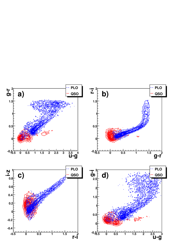
The photometric information is extracted from the SDSS-DR7 imaging database (Abazajian, 2009). The 10 elementary variables are the PSF magnitudes for the 5 SDSS bands () and their errors. As explained in Richards et al. (2009b), the most powerful variables are the four usual colors (,,,) which combine the PSF magnitudes. Fig. 1 shows the 2D color-color distributions for the QSO and PLO samples.
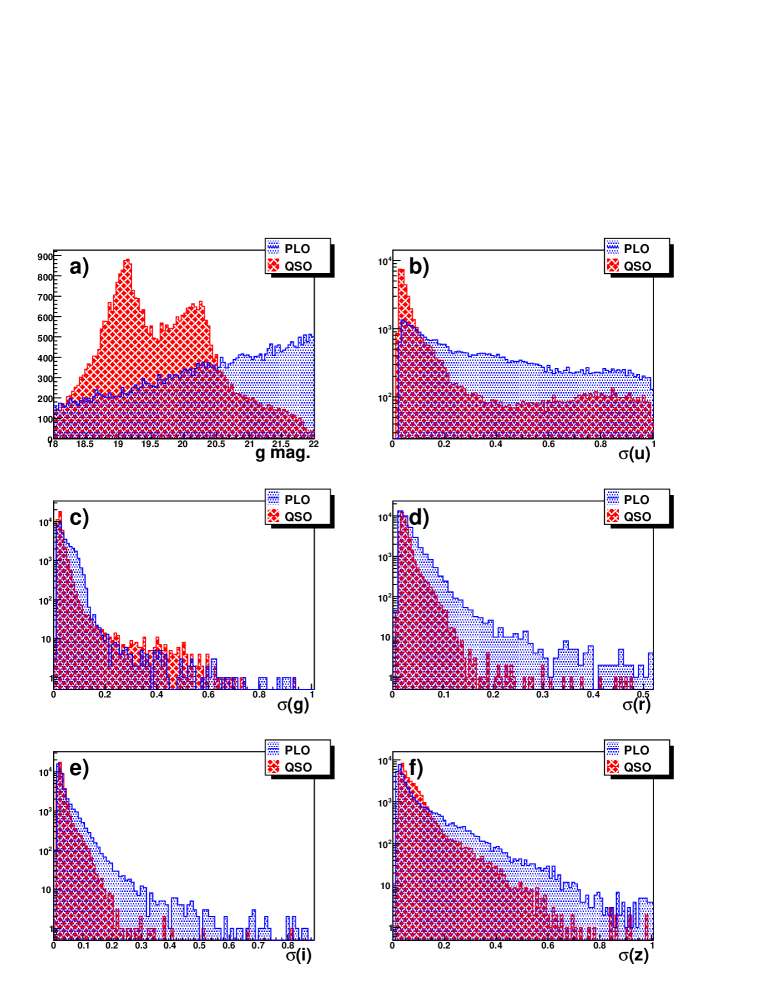
These plots give the impression that it is easy to disentangle the two classes of objects but one needs to keep in mind that the final goal is to obtain a 50% efficiency for QSOs with a non-quasar PLO efficiency of the order of . Therefore to improve the NN performances, we added the absolute magnitude and the five magnitude errors. Their distributions for the two classes are given on Fig. 2. An improvement can be expected from the additional variables and also from the correlations between the variables. Indeed, for example, it is expected that errors be larger for compact galaxies compared to intrinsic point-like objects.
Note that the distribution for the QSOs is likely to be biased by the spectroscopic selection. This issue will be addressed in the future with the first observations of BOSS. Indeed the photometric selection of QSOs for these first observations is based on loose selection criteria and it should provide a “less biased” catalog of spectroscopically confirmed quasars, close to completeness up to .
3 Neural Network Approach
The basic building block of the NN architecture 111 For this study, both for target selection and redshift determination, we use a C++ package, TMultiLayerPerceptron developed in the ROOT environment (Brun et al., 1995). is a processing element called a neuron. The NN architecture used in this study is illustrated in Fig. 3 where each neuron is placed on one of four “layers”, with neurons in layer . The output of each neuron on the first (input) layer is one of the variables defining an object, e.g. magnitudes, colors and uncertainties. The inputs of neurons on subsequent layers () are the outputs of the previous layer, i.e. the . The inputs of any neuron are first linearly combined according to “weights”, and “offsets”
| (1) |
The output of neuron on layer is then defined by the non-linear function
| (2) |
The fourth layer has only one neuron giving an output , reflecting the likelihood that the object defined by the input variables is a QSO.


Certain aspects of the NN procedure, especially the number of layers and the number of nodes per layer, are somewhat arbitrary and are chosen by experience and for simplicity. On the other hand, the weights and offsets must be optimized so that the NN output, , correctly reflects the probability that an input object is a QSO. The NN must therefore be “trained” with a set of objects that are known to be QSOs or not QSOs (background objects). More precisely, the weights and offsets are determined by minimizing the “error” function
| (3) |
where the sum is over objects, , and where is a discrete value defined as (resp. ) if the object is a QSO (resp. is not a QSO). In the case of the NN developed to estimate a photometric redshift, the targeted value is a continuous value equal to the true spectrometric redshift, . Note that in the NN architecture used for this study, the activation function, defined in Eq. 2, is not applied to the last neuron, allowing the output variable to vary in a range wider than .
In this kind of classification analysis, the major risk is the “over-training” of the NN. It occurs when the NN has too many parameters ( and ) determined by too few training objects. Over-training leads to an apparent increase in the classification efficiency because the NN learns by heart the objects in the training sample. To prevent such a behavior, the QSO and background samples are split into two independent sub-samples, called “training” and “control” samples. The determination of the NN parameters ( and ) is obtained by minimizing the error , computed over the QSO and background training samples. The minimization is suspended as soon as the error for the control samples stops decreasing even if the error is still decreasing for the training samples. We have followed this procedure both for the target selection and the determination of the photometric redshift.
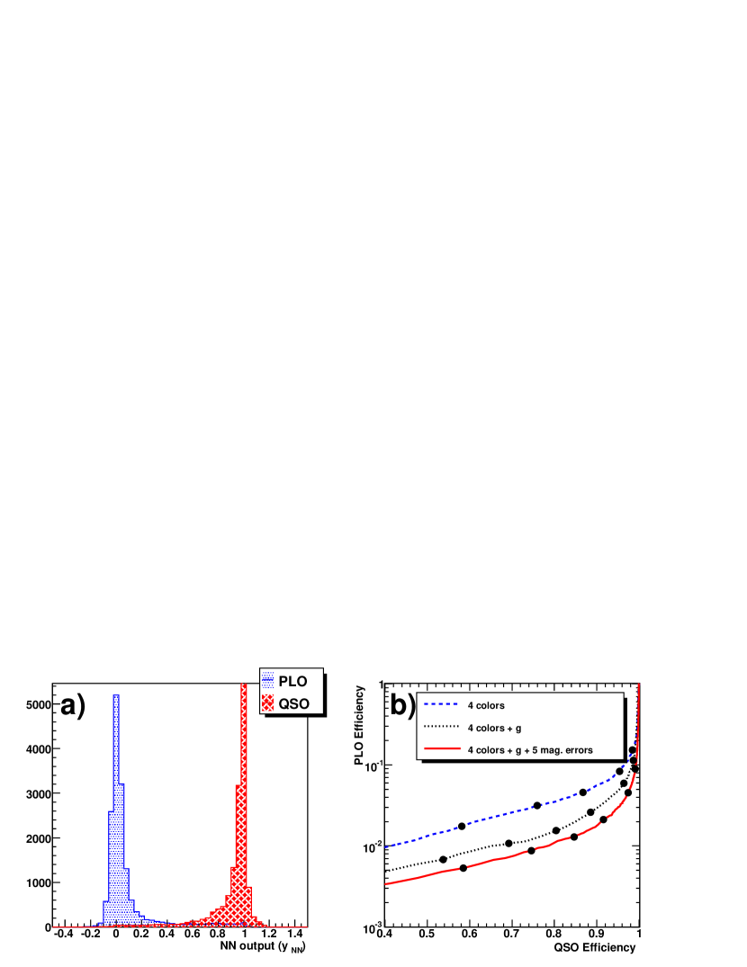
The result of the NN training procedure is shown in Fig. 4-a. The histograms of for the control QSO and background samples are overplotted. Most objects have either (corresponding to QSOs) or (corresponding to background objects). QSO target selection is achieved by defining a threshold value to be chosen between and . The optimal value of the threshold is obtained by balancing the number of accepted QSOs against the number of accepted background objects. A plot of the QSO efficiency vs. the background efficiency is shown in Fig. 4-b.
4 Photometric Selection of Quasar
For illustration, we have considered three NN configurations that differ by the number of discriminating variables. The first one uses only the four standard colors (,,,). In the second configuration, we add the absolute magnitude and finally in the third configuration, the errors on the five PSF magnitudes are also taken into account. For each configuration, we have optimized the number of neurons in the hidden layers and the number of iterations in the minimization to get the best “PLO efficiency–QSO efficiency” curve. The three curves are superimposed on Fig. 4-b. Adding information, i.e discriminating variables, clearly improves the classification performances. For instance, for a QSO efficiency of 50%, the PLO rejection fraction increases from 98.8%, to 99.4% and to 99.6% when the number of variables increases respectively from 4 to 5 and to 10. In the region of QSO efficiency in which we want to work, between 50% and 80%, the PLO background is reduced by a factor 3 by adding 6 variables to the four usual colors. The small improvement found by using photometric errors may be due to a small contamination of the PLO catalog by compact galaxies.
It is therefore apparent that the 10-variable NN should be used for the purpose of selecting quasars in any photometric catalog. In that case, the PLO rejection factors are respectively, 99.6%, 99.2% and 98.5% for QSO efficiencies of 50%, 70% and 85%.

According to the McDonald & Eisenstein (2007) computation based on the Jiang et al. (2006) survey of faint QSOs, we expect 20 QSOs per deg2, with and . For a galactic latitude , the number of objects selected in the SDSS-DR7 imaging database is 4000. Thus, with a QSO efficiency of 70% and a PLO efficiency222Note that by its definition in Sec.2.1, the PLO sample contains QSOs. of 0.8%, we will select 32 objects per deg2 including 14 “true” QSOs. These numbers corresponds roughly to what is required for BOSS project.
5 Photometric Redshift of Quasar
For the BOSS project, only quasars with a redshift in the range are useful. In the definition of the training sample, we have already applied a cut on the redshift, , to reinforce the selection of high- QSOs. But it is useful to add an additional constrain and select only QSOs with . This a-posteriori color cut helps to remove QSOs in the region . However, we propose a more elegant method which consists of estimating the redshift of the QSO from the photometric information with another NN.
For the determination of the photometric redshift we use the same 10 variables as those in the NN for target selection. The difference is that in the definition of the error , in Eq. 3, the targeted value is a continuous value equal to the true spectrometric redshift, . Except for this difference, the NN architecture is the same as for target selection with two hidden layers with the same number of hidden neurons. The minimization is computed with a single “training” sample of spectroscopically-confirmed QSOs and it is suspended as soon as the error for the QSO “control” sample stops decreasing.
Fig. 5-a shows the photometric redshift , determined with the NN versus the spectroscopic redshift of the spectroscopically-confirmed QSOs. Most of the objects are distributed along the diagonal demonstrating the good agreement between the two measurements. This can be quantified by plotting the difference (Fig. 5-b). The fit of this distribution with three gaussians gives and of the objects respectively in core and wide Gaussians. The fraction of outliers, determined with the third Gaussian is only .
The corresponding distribution can be fitted with three Gaussian functions comprizing, respectively, , and 0.2% of the distribution and of width, = 0.1, 0.4 and 1.
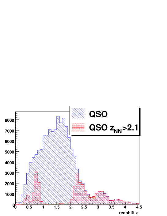
Therefore, as shown on Fig. 6, by applying a conservative cut on the photometric redshift, , we can remove 90.0% of the QSOs with . The fraction of lost QSOs with a redshift in the relevant region, , stays at a reasonable level of 5.3%.

6 Conclusions
In this paper we have presented a new promising approach to select quasars from photometric catalogs and to estimate their redshift. We use an Neurone Network with a multilayer perceptron architecture. The input variables are photometric measurements, i.e. the magnitudes and their errors for the five bands () of the SDSS photometry.
For the target selection, we achieve a PLO rejection factor of 99.6% and 98.5% for, respectively, a quasar efficiency of 50% and 85%. The rms of the difference between the photometric redshift and the spectroscopic redshift is of the order of 0.15 over the region relevant for BAO studies. These new statistical methods developed in the context of the BOSS project can easily be extended to any other analysis requiring QSO selection and/or determination of their photometric redshift.
Acknowledgements.
We thank N. P. Ross and D. H. Weinberg for triggering our interest in QSO target selection in the context of the BOSS project and for many interesting discussions. The authors are also grateful to G. T. Richards, A. D. Myers and E. Sheldon for important discussions and for providing the QSO catalog developed for the target selection in BOSS and used in this paper. We like also to thank Fan X. who has provided us some synthetic catalogs of PLOs.References
- Adelman-McCarthy et al. (2008) Adelman-McCarthy, J. K., et al., 2008, ApJS, 175, 297
- Abazajian (2009) Abazajian, K. N. et al., (the Seventh Data Release of the SDSS), 2009, ApJS, 182, 543
- Bishop (1995) Bishop, C. M., “Neural Networks for pattern recognition,” 1995, Oxford University Press
- Brun et al. (1995) Brun, R. et al., (the ROOT Team)http://root.cern.ch
- Caucci et al. (2008) Caucci, S. et al., 2008, MNRAS, 386, 211
- Cole et al. (2005) Cole, S. et al., (the 2dFGRS Team), MNRAS, 362, 505
- Croft et al. (1999) Croft, R. A. C. et al., 1999, ApJ, 520, 1
- Croom et al. (2001) Croom, S. M. et al., 2001, MNRAS, 322, 29
- Croom et al. (2004) Croom, S. M. et al., 2004, MNRAS, 349, 1397
- Croom et al. (2009) Croom, S. M. et al., 2009, MNRAS, 392, 19
- Eisenstein et al. (2005) Eisenstein, D. J. et al., (the SDSS Collaboration), 2005 ApJ, 633, 560
- Fan (1999) Fan, X. 1999, AJ, 117, 2528
- Jiang et al. (2006) Jiang, X. et al., 2006, AJ, 131, 2788
- Lupton et al. (1999) Lupton, R. H., Gunn J. E., Szalay A. S., 1999, AJ, 118, 1406
- McDonald & Eisenstein (2007) McDonald, P. and Eisenstein, D. J., 2007, Phys. Rev. D, 76, 063009
- Nusser &Haehnelt, (1999) Nusser, A. & Haehnelt, M., 1999, MNRAS, 303, 179
- Oke & Gunn (1983) Oke, J. B., Gunn, J. E., 1983, ApJ, 266, 713
- Percival et al. (2009) Percival, W. J. at al., 2009, submitted to MNRAS, arXiv:0907.1660
- Petitjean (1997) Petitjean, P., “The Early Universe with the VLT”, edited by Jacqueline Bergeron 1997, Berlin, Springer, 266
- Pichon et al. (2001) Pichon, C. et al., 2001, MNRAS, 326, 597
- Richards et al. (2001) Richards, G. T. et al., 2009, AJ, 122, 1151
- Richards et al. (2004) Richards, G. T. et al., 2004, ApJS, 155, 257
- Richards et al. (2009a) Richards, G. T. et al., AJ, 137, 3884
- Richards et al. (2009b) Richards, G. T. et al., 2009, ApJS, 180, 67
- Schlegel et al. (1998) Schlegel, D. J., Finkbeiner, D. P., Davis, M., 1998, ApJ, 500, 525
- Schlegel, White & Eisenstein (2009) Schlegel, D., White, M., and Eisenstein, D., 2009, arXiv:0902.4680
- Schmidt (1963) Schmidt, J. A. 1963, Nature, 197, 1040
- SDSS-III Coll. (2008) SDSS-III Collaboration, http://www.sdss3.org/collaboration/description.pdf
- Shanno (1970) Shanno, D. F., 1970, Math. Comp., 24, 647
- Weinstein et al. (2004) Weinstein, M. A. et al., 2004, ApJS, 155, 243