On the Absence of Photospheric Net Currents in Vector Magnetograms of Sunspots Obtained From Hinode (SOT/SP)

Abstract

Various theoretical and observational results have been reported regarding the presence/absence of net electric currents in the sunspots. The limited spatial resolution of the earlier observations perhaps obscured the conclusions. We have analyzed 12 sunspots observed from Hinode (SOT/SP) to clarify the issue. The azimuthal and radial components of magnetic fields and currents have been derived. The azimuthal component of the magnetic field of sunspots is found to vary in sign with azimuth. The radial component of the field also varies in magnitude with azimuth. While the latter pattern is a confirmation of the interlocking combed structure of penumbral filaments, the former pattern shows that the penumbra is made up of a “curly interlocking combed” magnetic field. The azimuthally averaged azimuthal component is seen to decline much faster than 1/$\varpi$ in the penumbra, after an initial increase in the umbra, for all the spots studied. This confirms the confinement of magnetic fields and absence of a net current for sunspots as postulated by Parker (1996). The existence of a global twist for a sunspot even in the absence of a net current is consistent with a fibril-bundle structure of the sunspot magnetic fields.

1 Introduction

Sunspots have shown evidence for twist even from the time of Hale (1925, 1927) who postulated the hemispheric rule for the chirality of chromospheric whirls. This was later confirmed with a larger data set by Richardson (1941). Evidence for photospheric chirality could be seen in early continuum images of sunspots, obtained with exceptional image quality. Later, photospheric vector magnetograms showed global twist inferred from the non-vanishing averages of the force-free parameter (Pevtsov et al. (1994); Hagino & Sakurai (2004); Nandy (2006) and references therein). The non-force-free nature of photospheric magnetic field in the sunspots, prompted Tiwari et al. (2009a) to propose the signed shear angle (SSA) as a more robust measure of the global twist of the sunspot magnetic field.

Although, the sign of SSA matches well with the sign of the global alpha parameter, the magnitudes are not so well correlated. The physical significance of a globally averaged $\alpha$ parameter rests heavily on the existence of a net current in the photospheric sunspot magnetic field. One way of arriving at a global $\alpha$ is by taking the ratio of total vertical current to the total flux (integral method). This value was found to agree with the values obtained by other methods (Hagino & Sakurai, 2004).

For a monolithic sunspot magnetic field, the global twist and net current is expected to be well correlated by Ampere’s Law. However, the existence of a net current is ruled out theoretically for fibril bundles as well as for monolithic fields with azimuthal field decreasing faster than 1/$\varpi$, where $\varpi$ is the radial distance from the spot center (Parker, 1996). Several attempts to resolve this problem using vector magnetograms have not been very conclusive so far (Wilkinson et al., 1992; Leka et al., 1996; Wheatland, 2000).

A resolution of this problem can be used to disentangle the relation between global twist and the global $\alpha$ parameter. Also, the resolution is needed to evaluate the so called hemispheric helicity rule seen in the global $\alpha$ parameter calculated from photospheric vector magnetograms (Pevtsov et al., 1994, 1995; Hagino & Sakurai, 2004; Nandy, 2006). The availability of high resolution vector magnetograms from Hinode (SOT/SP), gives us the best opportunity so far to address this problem. The effect of polarimetric noise is expected to be negligible in the estimation of magnetic parameters (Tiwari et al., 2009b) from these data.

In this Letter we obtain an expression for the net current using a generalization of the expression obtained by Parker (1996). We then proceed to measure this current from several vector magnetograms of nearly circular sunspots. We finally discuss the results and present our conclusions.

2 Expression For Net Current

Following Parker (1996), we consider a long straight flux bundle surrounded by a region of field free plasma. We use the words “field free” in the empirical sense that there is no large scale coherent and unipolar magnetic field surrounding the flux bundle. Also, we include the case where the bundle can be replaced by a monolithic field. Parker (1996) assumed azimuthal symmetry as well as zero radial component $B_{r}$, of the magnetic field. For realistic sunspot fields, we need to relax both these assumptions.

The vertical component of the electric current density consists of two terms, viz. $-\frac{1}{\mu_{0}r}\frac{\partial B_{r}}{\partial\psi}$  and  $\frac{1}{\mu_{0}r}\frac{\partial(rB_{\psi})}{\partial r}$. We will call the first term as the “pleat current density”, $j_{p}$ and the second term as the “twist current density”, $j_{t}$. The net current $I_{z}$ within a distance $\varpi$ from the center is then given by

$$I_{z}(\varpi)=\int_{0}^{2\pi}d\psi\int_{0}^{\varpi}rdr(j_{p}+j_{t})$$ (1)

The $\psi$ integral over $j_{p}$ vanishes, while the second term yields

$$I_{z}(\varpi)=\frac{\varpi}{\mu_{0}}\int d\psi B_{\psi}(\varpi,\psi)$$ (2)

which gives the net current within a circular region of radius $\varpi$.

3 The Data Sets and Analysis

We have analyzed the vector magnetograms obtained from Solar Optical Telescope/Spectro-polarimeter (SOT/SP: Tsuneta et al. (2008); Shimizu et al. (2008); Suematsu et al. (2008); Ichimoto et al. (2008)) onboard Hinode (Kosugi et al., 2007). The calibration of data sets have been performed using the standard “SP_PREP” routine developed by B. Lites and available in the Solar-Soft package. The prepared polarization spectra have been inverted to obtain vector magnetic field components using an Unno-Rachkowsky (Unno, 1956; Rachkowsky, 1967) inversion under the assumption of Milne-Eddington (ME) atmosphere (Landolfi & Landi Degl’Innocenti, 1982; Skumanich & Lites, 1987). We have used the inversion code “STOKESFIT” which has been kindly made available by T. R. Metcalf as a part of the Solar-Soft package. We have used the newest version of this code which returns true field strengths along with the filling factor. The azimuth determination has inherent 180^o ambiguity due to insensitivity of Zeeman effect to orientation of the transverse fields. Numerous techniques have been developed and applied to resolve this problem, but not even one guarantees a complete resolution. The 180^o azimuthal ambiguity in our data sets are removed by using acute angle method (Harvey, 1969; Sakurai et al., 1985; Cuperman et al., 1992).

In order to minimize the noise, pixels with transverse $(B_{t})$ and longitudinal magnetic field $(B_{z})$ greater than a certain level are only analyzed. A quiet Sun region is selected for each sunspot and 1$\sigma$ standard deviation in the three vector field components $B_{x}$, $B_{y}$ and $B_{z}$ are evaluated separately. The resultant standard deviations of $B_{x}$ and $B_{y}$ is then taken as the 1$\sigma$ noise level for transverse field components. Only those pixels where longitudinal and transverse fields are simultaneously greater than twice the above mentioned noise levels are analyzed. The data sets with their observation details are given in Table 1. We have treated each polarity as an individual sunspot whenever both the polarities are observed and compact enough to be studied. We have studied only those spots where the polarity inversion lines are well separated from the edge of the sunspot.

The results of the inversions yield the 3 magnetic parameters, viz. the field strength B, the inclination to the line of sight $\gamma$, and the azimuth $\phi$. These parameters are used to obtain the 3 components of magnetic field in Cartesian geometry as

$$B_{z}=B\cos\gamma$$ (3)

$$B_{y}=B\sin\gamma\sin\phi$$ (4)

$$B_{x}=B\sin\gamma\cos\phi$$ (5)

This vector field is transformed to heliographic coordinates (Venkatakrishnan & Gary, 1989) for the spots observed at viewing angle more than $10^{\circ}$. The transverse vector is then expressed in cylindrical geometry as

$$B_{r}=\frac{1}{r}(xB_{x}+yB_{y})$$ (6)

$$B_{\psi}=\frac{1}{r}(-yB_{x}+xB_{y})$$ (7)

The azimuthal field $B_{\psi}$ is then used in equation (2) for obtaining the value for the total vertical current within a radius $\varpi$.

We have computed “twist angle” for all the sunspots using $B_{\psi}$ and $B_{r}$ as shown in Table 1. The error in “twist” measurement is simply the error in azimuth measurement. Using the weak field approximation, we can find the azimuth $\psi$ from $\tan 2\psi=U/Q$. From this we can estimate the error in $\psi$ as equal to the percentage error in linear polarization measurements. Thus, a 1% error in polarimetry means that the error in $\psi$ equals 0.01 radians or 0.57 degrees. We have performed Monte Carlo simulations of the effect of noise on the inversions which we plan to present in a more detailed paper. We have verified that the error in $\psi$ is consistent with the value estimated from the weak field approximation.

We can see in the Table 1 that the twist angles for regular sunspots match well with the global SSA as expected, whereas they do not match for irregular sunspots.

4 The Results

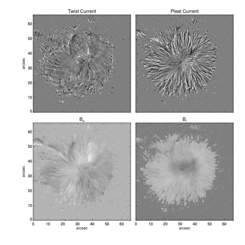
Figure 1: Examples of the two components of the vertical electric current density namely the “twist” and the “pleat” current densities ($j_{t}$ and $j_{p}$) observed in NOAA AR 10933 are shown in the upper panel. The lower panel shows the azimuthal and radial component of the magnetic field ($B_{\psi}$ and $B_{r}$).

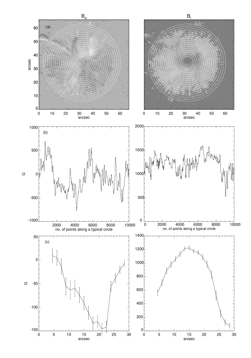
Figure 2: (a): The same image as the lower panel of Figure 1 but with concentric circles over plotted on them. (b): Plots of $B_{\psi}$ and $B_{r}$ along the periphery of a typical circle (45^th pixel away from center) selected in the sunspot. (c): The mean $B_{\psi}$ and mean $B_{r}$ with $\frac{1}{16}$ and $\frac{1}{8}$ of their variations respectively along radial direction with different $\varpi$ have been plotted.

Figure 1 shows an example of the maps of twist current, pleat current, $B_{\psi}$ and $B_{r}$ for a sunspot NOAA AR 10933 which is nearly circular. Figure 2(a) shows plots of $B_{\psi}$ and $B_{r}$ along with the different concentric circles around spot center. In Figure 2(b), the spatial variation of both $B_{\psi}$ and $B_{r}$ are clearly seen. This variation is corresponding to a typical circle selected in the penumbra. The $B_{r}$ variation in the penumbra is a manifestation of the interlocking combed structure (Ichimoto et al., 2007; Tiwari et al., 2009a). The $B_{\psi}$ variation in the penumbra shows that not only is there an interlocking combed structure, but these structures are curled as well. In other words, we may describe the penumbral field as possessing a “curly interlocking combed” structure. This feature of the deviation of the vector field azimuths from a radial direction was also seen by Mathew et al. (2003) in the magnetic field of a sunspot belonging to NOAA AR 8706, using the infra-red FeI line pair at 1.56 micron.

The azimuthal averages $<B_{\psi}>$ and $<B_{r}>$ were obtained at different values of $\varpi$. Figure 2(c) shows the plots of $<B_{\psi}>$ and $<B_{r}>$ as a function of $\varpi$. The circles corresponding to the selected radii are shown in the upper panel of the same figure. The azimuth-averaged $<B_{r}>$ drops rapidly to a very low value at the edge of the sunspot. This is a clear evidence for the existence of a canopy where the field lines lift up above the line forming region. Figure 3 shows the plot of log $<B_{\psi}>$ as a function of log $\varpi$. The slope $\delta$ of the declining portion of this plot is 9.584, which shows that field varies faster than 1/$\varpi$. This can be construed as evidence for the neutralization of the net current. The $\delta$ for other sunspots have also been computed and are given in Table 1.

The map of vertical current density j_z for the same sunspot is shown with intensity scale in the left panel of Figure 4. The values are expressed in Giga Amperes per square meter (GA/m²). We can see that the distribution of j_z is dominated by high amplitude fluctuations on small scale as also reported in Tiwari et al. (2009a). It is therefore difficult to make out any systematic behaviour of the sign of j_z as a function of $\varpi$.

The right panel of the same figure shows the total current within a radius $\varpi$ as a function of $\varpi$. As expected from the trend in Figure 3, the total current shows evidence for a rapid decline after reaching a maximum. Similar trends were seen in other sunspots. We have also plotted in right panel of Figure 4, the net current as calculated by the derivative method (viz. summation of current densities calculated as the local curl of B). We do see a trend of neutralization, although the effect is less pronounced because of the larger noise present in the derivative method. We can also infer from the right panel of Figure 4 that the increments of net vertical current flowing through annular portions of the sunspot do show a reversal in sign.

Table 1 shows the summary of results for all the sunspots analyzed. Along with the power law index $\delta$ of $B_{\psi}$ decrease, we have also shown the average deviation of the azimuth from the radial direction (“twist angle”), as well as the SSA. The average deviation of the azimuth is well correlated with the SSA for nearly circular sunspots, but is not correlated with SSA for more irregularly shaped sunspots. Thus, SSA is a more general measure of the global twist of sunspots, irrespective of their shape.

5 Discussion and Conclusions

It is well known for astrophysical plasmas, that the plasma distorts the magnetic field and the curl of this distorted field produces a current by Ampere’s law (Parker, 1979). Parker’s (1996) expectation of net zero current in a sunspot was chiefly motivated by the concept of a fibril structure for the sunspot field. However, he also did not rule out the possibility of vanishing net current for a monolithic field where the azimuthal component of the vector field in a cylindrical geometry declines faster than 1/$\varpi$. While it is difficult to detect fibrils using the Zeeman effect notwithstanding the superior resolution of SOT on Hinode, the stability and accuracy of the measurements have allowed us to detect the faster than 1/$\varpi$ decline of the azimuthal component of the magnetic field, which in turn can be construed as evidence for the confinement of the sunspot field by the external plasma. The resulting pattern of curl B appears as a drop in net current at the sunspot boundary.

If this lack of net current turns out to be a general feature of sunspot magnetic fields in the photosphere, then measurement of helicity from a global average of the force-free parameter becomes suspect. On the other hand, sunspots are evidently twisted at photospheric levels, as seen from the non-vanishing average twist angle as well as the SSA (Table 1). Although the existence of a global twist in the absence of a net current is possible for a monolithic sunspot field (Baty, 2000; Archontis et al., 2004; Fan & Gibson, 2004; Aulanier et al., 2005), a fibril model of the sunspot field can accommodate a global twist even without a net current (Parker, 1996).

The spatial pattern of current density in a sunspot (e.g., left panel of Figure 4) is really a manifestation of the deformation of the magnetic field ($\nabla\times\bf B$) by the forces applied by the plasma. The Lorentz force exerted by the field on the plasma produces an equal and opposite force by the plasma, thereby confining the field. Thus our analysis actually shows the pattern of the forces exerted by the plasma on the field. The sharp decline of the azimuthal field with radial distance thus shows the confinement of the sunspot magnetic field by the radial gradient of the plasma pressure.

Theoretical understanding of the penumbral fine structure has improved considerably in recent times (Thomas et al., 2002; Weiss et al., 2004). The onset of a convective instability for magnetic field inclination exceeding a critical value was proposed by Tildesley (2003) and Hurlburt et al. (2002). A bifurcation in the onset (Rucklidge et al., 1995) could explain other features like hysteresis in the appearance of penumbra as a function of sunspot size. Numerical simulation of magneto-convection also steadily improved (Heinemann et al., 2007; Rempel et al., 2009a), culminating in very realistic production of penumbral field structure (Rempel et al., 2009b). It is possible, owing to the random and stochastic nature of convective structures, that no net twist in the simulated spot field would be produced by convection for negligible Coriolis force. If so, it would be very interesting to simulate magneto-convection in a twisted sunspot field. In this case, would the resulting fine structure mimic the observed “curly interlocking combed” structure of the penumbral magnetic field? If not, we must look elsewhere for explaining the “curly interlocking combed” structure. A twisted fibril bundle would then be a solution. Recent examples of filamentary penumbral structures based on such cluster models (Solanki & Montavon, 1993; Spruit & Scharmer, 2006; Scharmer & Spruit, 2006) have also been proposed.

Parker (1996) also mentions the possibility of net currents in the corona, continuing down to the height where the first cleaving takes place. It would therefore be imperative to look for net currents at higher reaches of the solar atmosphere. This is very important because several theories of flares (Melrose, 1995) and CME triggers (Forbes & Isenberg, 1991; Kliem & Török, 2006) rely heavily on the existence of net currents in the corona above the sunspots.

Future large ground based telescopes equipped with adaptive optics and multi spectral line capabilities would go a long way in addressing these issues. In the meantime, direct measurement of the global twist of sunspots using parameters like the SSA should serve as proxies for estimating the net currents of active regions in the corona. The SSA will also be a better parameter to base a fresh look at the hemispheric rule in photospheric chirality.

Table 1: List of the active regions studied. The power index $\delta$: the slope of decrease of $B_{\psi}$ value, the twist angle, the signed shear angle (SSA) and other details of the sunspots are given:

AR No.	Date of	Slope	Shear Angle	Twist Angle	Position	Hemispheric
(NOAA)	Observation	$\delta$	(SSA: deg)	$(tan^{-1}(B_{\psi}/B_{r})$: deg)		Helicity Rule
10969	29 Aug 2007	$7.514$	$-4.488$	$-4.009$	S05W33(t)	No
10966	07 Aug 2007	$4.349$	$-5.120$	$-7.028$	S06E20(t)	No
10963($-$)	12 Jul 2007	$4.366$	$-5.123$	$41.873^{\sharp}$	S06E14(t)	No
10963($+$)	12 Jul 2007	$4.210$	$-4.495$	$-5.112$	S06E14(t)	No
10961	02 Jul 2007	$4.976$	$-4.973$	$29.451^{\sharp}$	S10W16(t)	No
10960	07 Jun 2007	$3.267$	$3.182$	$-24.012^{\sharp}$	S07W03	Yes
10953	29 Apr 2007	$8.249$	$-3.382$	$7.200^{\sharp}$	S10E22(t)	No
10944	03 Mar 2007	$2.407$	$-4.635$	$-5.130$	S05W30(t)	No
10940	01 Feb 2007	$2.281$	$-4.726$	$-7.950$	S04W05	No
10933	05 Jan 2007	$9.584$	$-2.283$	$-2.689$	S04W01	No
10926	03 Dec 2006	$2.750$	$-1.538$	$6.001^{\sharp}$	S09W32(t)	No
10923	10 Nov 2006	$3.175$	$0.785$	$-9.010^{\sharp}$	S05W30(t)	Yes

Figure 3: Variation of log $<B_{\psi}>$ with log $\varpi$. The slope of the declining portion of plot has been calculated as a simple power law index $\delta$ for each sunspot and has been given in Table 1.

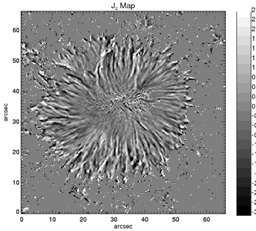
Figure 4: Left panel: The map of vertical current density j_z is shown with intensity scale. The values are expressed in Giga Amperes per square meter (GA/m²). Right panel: The net current variation with increasing area has been shown. The solid line shows the results of the calculations from the Equation 2. Also shown, by a dashed line, is the results from the derivative method. We can see the net current reduces very fast after a peak and almost vanishes for complete sunspot. On the other hand the net current computed from the derivative method shows a shallow behaviour.

References

- Archontis et al. (2004) Archontis, V., Moreno-Insertis, F., Galsgaard, K., Hood, A., & O’Shea, E. 2004, A&A, 426, 1047
- Aulanier et al. (2005) Aulanier, G., Démoulin, P., & Grappin, R. 2005, A&A, 430, 1067
- Baty (2000) Baty, H. 2000, A&A, 360, 345
- Cuperman et al. (1992) Cuperman, S., Li, J., & Semel, M. 1992, A&A, 265, 296
- Fan & Gibson (2004) Fan, Y., & Gibson, S. E. 2004, ApJ, 609, 1123
- Forbes & Isenberg (1991) Forbes, T. G., & Isenberg, P. A. 1991, ApJ, 373, 294
- Hagino & Sakurai (2004) Hagino, M., & Sakurai, T. 2004, PASJ, 56, 831
- Hale (1925) Hale, G. E. 1925, PASP, 37, 268
- Hale (1927) Hale, G. E. 1927, Nature, 119, 708
- Harvey (1969) Harvey, J. W. 1969, Ph.D. thesis, AA(University of Colorado at Boulder.)
- Heinemann et al. (2007) Heinemann, T., Nordlund, Å., Scharmer, G. B., & Spruit, H. C. 2007, ApJ, 669, 1390
- Hurlburt et al. (2002) Hurlburt, N. E., Alexander, D., & Rucklidge, A. M. 2002, ApJ, 577, 993
- Ichimoto et al. (2008) Ichimoto, K., et al. 2008, Sol. Phys., 249, 233
- Ichimoto et al. (2007) Ichimoto, K., et al. 2007, PASJ, 59, 593
- Kliem & Török (2006) Kliem, B., & Török, T. 2006, Physical Review Letters, 96, 255002
- Kosugi et al. (2007) Kosugi, T., et al. 2007, Sol. Phys., 243, 3
- Landolfi & Landi Degl’Innocenti (1982) Landolfi, M., & Landi Degl’Innocenti, E. 1982, Sol. Phys., 78, 355
- Leka et al. (1996) Leka, K. D., Canfield, R. C., McClymont, A. N., & van Driel-Gesztelyi, L. 1996, ApJ, 462, 547
- Mathew et al. (2003) Mathew, S. K., et al. 2003, A&A, 410, 695
- Melrose (1995) Melrose, D. B. 1995, ApJ, 451, 391
- Nandy (2006) Nandy, D. 2006, Journal of Geophysical Research (Space Physics), 111, 12
- Parker (1979) Parker, E. N. 1979, Cosmical magnetic fields: Their origin and their activity (Oxford, Clarendon Press; New York, Oxford University Press, 1979, Chapter 2)
- Parker (1996) Parker, E. N. 1996, ApJ, 471, 485
- Pevtsov et al. (1994) Pevtsov, A. A., Canfield, R. C., & Metcalf, T. R. 1994, ApJ, 425, L117
- Pevtsov et al. (1995) Pevtsov, A. A., Canfield, R. C., & Metcalf, T. R. 1995, ApJ, 440, L109
- Rachkowsky (1967) Rachkowsky, D. N. 1967, Izv. Krymsk. Astrofiz. Obs., 37, 56
- Rempel et al. (2009a) Rempel, M., Schüssler, M., & Knölker, M. 2009a, ApJ, 691, 640
- Rempel et al. (2009b) Rempel, M., Schüssler, M., Cameron, R. H., & Knölker, M. 2009b, Science, 325, 171
- Richardson (1941) Richardson, R. S. 1941, ApJ, 93, 24
- Rucklidge et al. (1995) Rucklidge, A. M., Schmidt, H. U., & Weiss, N. O. 1995, MNRAS, 273, 491
- Sakurai et al. (1985) Sakurai, T., Makita, M., & Shibasaki, K. 1985, MPA Rep., No. 212, p. 312 - 315
- Scharmer & Spruit (2006) Scharmer, G. B., & Spruit, H. C. 2006, A&A, 460, 605
- Shimizu et al. (2008) Shimizu, T., et al. 2008, Sol. Phys., 249, 221
- Skumanich & Lites (1987) Skumanich, A., & Lites, B. W. 1987, ApJ, 322, 473
- Solanki & Montavon (1993) Solanki, S. K., & Montavon, C. A. P. 1993, A&A, 275, 283
- Spruit & Scharmer (2006) Spruit, H. C., & Scharmer, G. B. 2006, A&A, 447, 343
- Suematsu et al. (2008) Suematsu, Y., et al. 2008, Sol. Phys., 249, 197
- Thomas et al. (2002) Thomas, J. H., Weiss, N. O., Tobias, S. M., & Brummell, N. H. 2002, Nature, 420, 390
- Tildesley (2003) Tildesley, M. J. 2003, MNRAS, 338, 497
- Tiwari et al. (2009a) Tiwari, S. K., Venkatakrishnan, P., & Sankarasubramanian, K. 2009a, ApJ, 702, L133
- Tiwari et al. (2009b) Tiwari, S. K., Venkatakrishnan, P., Gosain, S., & Joshi, J. 2009b, ApJ, 700, 199
- Tsuneta et al. (2008) Tsuneta, S., et al. 2008, Sol. Phys., 249, 167
- Unno (1956) Unno, W. 1956, PASJ, 8, 108
- Venkatakrishnan & Gary (1989) Venkatakrishnan, P., & Gary, G. A. 1989, Sol. Phys., 120, 235
- Weiss et al. (2004) Weiss, N. O., Thomas, J. H., Brummell, N. H., & Tobias, S. M. 2004, ApJ, 600, 1073
- Wheatland (2000) Wheatland, M. S. 2000, ApJ, 532, 616
- Wilkinson et al. (1992) Wilkinson, L. K., Emslie, A. G., & Gary, G. A. 1992, ApJ, 392, L39