Evidence of tidal debris from $\omega$ Cen in the Kapteyn Group

Abstract

This paper presents a detailed kinematic and chemical analysis of 16 members of the Kapteyn moving group. The group does not appear to be chemically homogenous. However, the kinematics and the chemical abundance patterns seen in 14 of the stars in this group are similar to those observed in the well-studied cluster, $\omega$ Centauri. Some members of this moving group may be remnants of the tidal debris of $\omega$ Cen, left in the Galactic disk during the merger event which deposited $\omega$ Cen into the Milky Way.

1 Introduction

The idea of hierarchical galaxy formation, in which galaxies are believed to form from the aggregation of smaller elements (see review by Freeman & Bland-Hawthorn (2002)), has been around since Searle & Zinn (1978) first proposed this theory as a challenge to the belief that galaxies formed through the smooth collapse of a large protocloud (Eggen et al., 1962). The identification of debris from these smaller fragments remains of utmost importance in modern studies of theoretical and observational stellar dynamics.

The most massive Galactic globular cluster, $\omega$ Cen, has several unique physical properties which suggest that there are very significant differences in star formation histories, enrichment processes and structure formation between $\omega$ Cen and other normal globular clusters (Bekki & Freeman, 2003).

A commonly accepted scenario of formation of $\omega$ Cen is that it is the surviving nucleus of an ancient dwarf galaxy, the outer envelope of which was entirely removed by tidal stripping as it was accreted by the Galaxy (Bekki & Freeman (2003) and references therein). Through numerical simulations, Bekki & Freeman (2003) demonstrated the dynamical feasibility of $\omega$ Cen forming from an ancient nucleated dwarf galaxy which was accreted into the young Galactic disk.

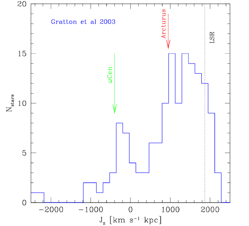
Figure 1: Distribution of specific angular momentum of all stars in the metal-poor compilation of Gratton et al. (2003). The excess of stars corresponding to the $\omega$ Cen group is evident. (Taken from Meza et al. 2005.)

Meza et al. (2005) used numerical simulations to investigate the characteristics of tidal debris from satellite galaxies. They showed that these satellites deposit a large fraction of their stars into either the disc component of the Milky Way or into the halo, showing distinct “trails” in the angular momentum – energy plane, depending on the plane of the satellite’s orbit during disruption. Meza et al. discussed the presence of the $\omega$ Cen stellar moving group (i.e. the stellar debris) in two studies of metal-poor stars in the solar neighbourhood, those of Beers et al. (2000) and Gratton et al. (2003). Figure 1 (taken from Meza et al. (2005)) shows how the $\omega$ Cen group is distinguished in the angular momentum distribution for the Gratton et al. (2003) sample. In both this sample and the Beers et al. (2000) sample, the $\omega$ Cen group appears as an over-density of stars at very specific rotational velocity or angular momentum values. The radial (U) velocities for the $\omega$ Cen candidate stars are observed to have a symmetric distribution, ranging from -300 to 300 km s^-1. An earlier simulation by Bekki & Freeman (2003) of the accretion of the $\omega$ Cen parent galaxy showed a strong plume of debris stars in the solar neighborhood with L_z near $-500$ kpc km s^-1. See also the discussion by Mizutani et al. (2003) on the kinematics of tidal debris from the parent galaxy.

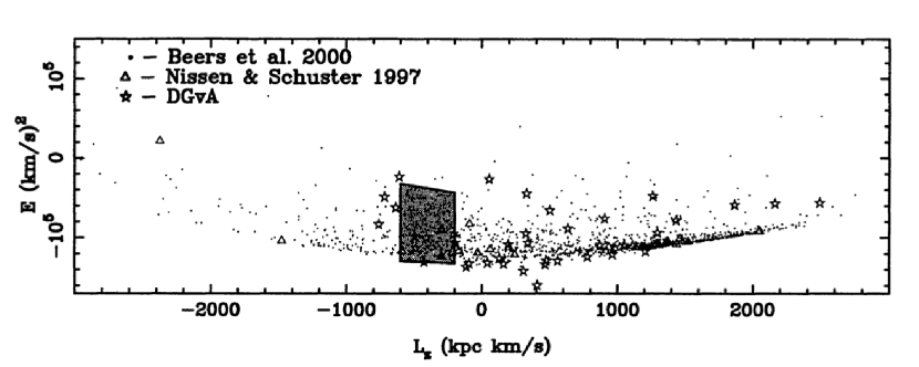
Figure 2: Orbital parameters for various studies of metal-poor stars in the solar neighbourhood. The candidate stars from $\omega$ Cen are chosen to lie in the shaded zone in the E-L_z plane. (Taken from Dinescu, 2002.)

Dinescu (2002) also provided a theoretical prediction of where the $\omega$ Cen group would appear kinematically using the metal-poor star sample of Beers et al. (2000). Figure 2 shows the angular momentum – energy plane, in which the shaded zone represents the area where expected $\omega$ Cen candidate stars would lie. Dinescu defines this region by assessing three globular clusters ($\omega$ Cen, NGC 362 and NGC 6779) that are believed to have come from the same original parent galaxy, and argues that their distribution may define the area in which further candidate remnants could lie. This region covers a large interval of energy over an angular momentum range from about L_z= -200 to -600 kpc km s^-1.

We have recently investigated the chemical properties of stars in the Kapteyn moving group, first introduced by Eggen (1962). The stars of the Kapteyn group, as most recently tabulated by Eggen (1996), are mostly metal-poor and in retrograde galactic orbits, so they were identified as a halo moving group. Moving stellar groups can originate in several ways. Some form from a common gas cloud. As the resulting cluster disperses, its stars dissolve into the Galactic background yet maintain some common kinematical identity which may be used to identify members of a particular stellar group. Such moving groups represent a transition between bound clusters and field stars, and are probably chemically homogeneous (see De Silva et al. (2007) and references therein). Other moving groups appear to result from resonances in the galactic disk (eg Dehnen (1998)), and others possibly as the debris of accreted and disrupted dwarf galaxies (Navarro et al., 2004). We were interested to see whether the Kapteyn group members were chemically similar, because this would be a pointer to the group’s origin. It turned out that some of the group stars show chemical peculiarities similar to those seen in $\omega$ Cen, and we will argue that the Kapteyn group may be part of the $\omega$ Cen debris.

Concentrations of metal-poor stars at L_z values near those of $\omega$ Cen and the Kapteyn group have appeared in several recent studies. Dettbarn et al. (2007) investigated substructure in a sample of stars with [Fe/H]$<-1$ from the Beers et al (2000) catalog and identified a structure (their feature K) which appears to be related to the Kapteyn star group. The study of 246 metal-poor stars with accurate kinematics by Morrison et al. (2009) also showed a substantial number of stars at weakly retrograde values of L_z, similar to that of $\omega$ Cen. Klement et al. (2009) find evidence of Kapteyn stream stars in their study of halo streams from the SDSS DR7.

This paper presents a kinematic and chemical analysis of 17 members of the Kapteyn moving group. Section 2 presents a kinematic analysis of the group. In Section 3 the observations and reduction procedures are outlined, and Section 4 gives the details of the chemical abundance study. The summary and conclusions are given in Section 5.

2 Kinematic Analysis

The initial 17 stars for this study were taken from Eggen (1996), which presents 33 Kapteyn group members. All non-binary southern sky members of the Kapteyn group were observed, except for the hottest candidates, defined as (B-V)${}_{\textrm{Eggen}}$ $<$ 0.40, which would have had few lines for analysis and the coolest stars, defined as (B-V)${}_{\textrm{Eggen}}$ $>$ 0.95, in which molecular features makes abundance analysis difficult.

Table 1 shows the basic kinematic data for each star. The proper motions are taken from the Hipparcos catalogue, radial velocities are taken from various sources (see notes to Table 1) and distances are taken from the Beers et al. (2000) catalogue. Three stars in this sample (BD -13 3834, G 18-54 and G 24-3) were not in the Beers et al. catalogue. For two of these stars, we used the method of Beers et al. 2000 to obtain distances consistent with those in the catalogue. The distances for G 18-54 and G 24-3 were found using

$M_{v}=-2.1576+19.9889(B-V)-15.0820(B-V)^{2}+4.7913(B-V)^{3}$

taken from Beers et al. (2000), using (B-V)=0.47 and 0.45 respectively (Eggen, 1996). This equation holds for all dwarf stars and was used to correspond to the dwarf gravities found for these stars via spectroscopic analysis (see Section 4 for details). The star BD -13 3834 was discarded from the sample due to the inability to obtain a reliable model atmosphere for this star (discussed further in Section 4). This, in turn, meant a reliable distance could not be found for this star, rendering any kinematics obtained for this object essentially meaningless. The remainder of the analysis was undertaken on only 16 stars.

In order to study the kinematics of this moving group, space motions were calculated using the parameters listed in Table 1. The U velocity is defined as positive toward the Galactic anti-center. The U, V and W velocities were corrected for the solar motion of (U, V, W)_sun = (-10.0, +5.2, +7.2 km s^-1) from Dehnen (1998), and are shown in Table 2. For consistency with the work of Dinescu et al. (1999), the energy and angular momentum were calculated using their adopted potential. This is based on the Paczynski (1990) Galactic model with an additional offset of $\Phi_{o}$=-12.3 x 10⁴, introduced in order to set the escape velocity at R = 8.0 kpc to be 500 km s^-1. The potentials used for the bulge, disk and dark halo are shown in Equations 3, 4 and 5 respectively.

$$\Phi_{b}=\frac{-GM_{b}}{\sqrt{R^{2}+(a_{b}+\sqrt{z^{2}+{b_{b}}^{2}})^{2}}}$$ (1)

$$\Phi_{d}=\frac{-GM_{d}}{\sqrt{R^{2}+(a_{d}+\sqrt{z^{2}+{b_{d}}^{2}})^{2}}}$$ (2)

$$\Phi_{h}=\frac{GM_{h}}{d}\left[\frac{1}{2}ln\left(1+\frac{r^{2}}{d^{2}}\right)+\frac{d}{r}arctan\frac{r}{d}\right]$$ (3)

The bulge and disk are modeled as modified Plummer potentials, as introduced by Miyamoto & Nagai (1975), while the dark halo is modeled as a logarithmic potential. The constants used in each Galactic model potential are given in Table 3. The resulting energy E and angular momentum L_z for each star in the sample are also given in Table 2. The Lindblad diagram (E vs L_z) was constructed, including our stars, stars from the Beers et al. catalog and the cluster $\omega$ Cen itself (see Table 4), to investigate whether there is any kinematic connection between $\omega$ Cen and the Kapteyn group. It was already evident that the E,L_z values for the Kapteyn group stars lie in the same retrograde region of the Lindblad diagram as $\omega$ Cen. The errors on E and L_z will be highly correlated for some stars, because both are dependent on distance. We ran Monte Carlo simulations for each star to estimate the error distributions of the derived E, L_z values. Errors adopted for V_rad, $\mu_{\alpha}$ and $\mu_{\delta}$ were those quoted in the various sources for each star. Errors on distance were set at 20$\%$, consistent with the error estimates on distance in the Beers et al. (2000) catalog. For each star, 1000 values were drawn from Gaussian probability distributions for V_rad, $\mu_{\alpha}$, $\mu_{\delta}$ and distance $d$, with $\sigma$ values for each equal to the errors discussed above. These values were then propagated through the calculation of U, V, W, E and L_z to obtain a probability distribution of these derived quantities for each star. These probability distributions show how tightly confined the stars are on the Lindblad diagram and, consequently, how likely the stars are to be kinematically related to $\omega$ Cen.

2.1 Kinematics Results

Table 2 gives the space velocities U,V,W and their error, the angular momentum L_z and the energy E for all stars in our sample. These stars were originally selected by Eggen (1996) because of their tightly confined range of V velocities, lying between $V=-275$ to $-300$ km s^-1. However, with modern parallaxes, radial velocities and proper motions, we find that Eggen’s Kapteyn group members in our study are still mostly in retrograde orbits but occupy a more extended area of phase-space than he found, with V values lying in a much larger range between $V=-115$ to $-368$ km s^-1. All stars in the sample show U values well within the range observed for the $\omega$ Cen candidate stars in the Meza et al. (2005) study. Meza et al found that all candidates had U values between -300 and 300 km s^-1 and a velocity dispersion greater than 200 km s^-1. The 16 stars in this sample of the Kapteyn group have U values between -177 and 172 km s^-1.

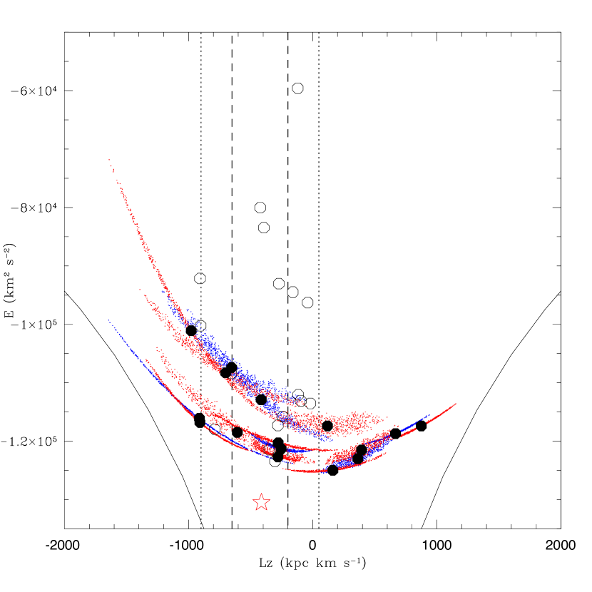
Figure 4: Lindblad diagram for Kapteyn group and Gratton peak. Symbols for the Kapteyn group stars and the Gratton peak stars, and the vertical lines, are as in Figure 3. The smaller dots represent the error distribution in E,L_z for the Kapteyn group stars, as discussed in the text. The different colors used are intended only to provide clarity between the distributions for different stars.

The Lindblad diagram is shown in Figure 3 for the Kapteyn group stars and several other samples. The large solid circles are for the retrograde Kapteyn group stars (given in Table 2). These stars appear again in Figure 4: the elongated cloud of smaller coloured points around each solid circle show the outcome of the Monte Carlo simulations discussed above. The points outline the 1$-\sigma$ or 68% confidence level for each Kapteyn group star. The clouds of Monte Carlo points are plotted in different colors to provide some clarity between the different stars and their uncertainties. As expected, the errors in L_z and E are highly correlated. The open red star is for $\omega$ Cen, using the parameters given in Table 4. The total uncertainties from a Monte Carlo simulation using errors in V_rad, $\mu_{\alpha}$, $\mu_{\delta}$ and distance for Omega Cen’s parameters are smaller than the starred symbol. The smaller green circles are stars from the Beers et al. catalogue, with an [Fe/H] filter applied to cover $-2.5<$ [Fe/H $<-0.5$, the abundance range observed in $\omega$ Cen. The region in which Dinescu (2002) suggested that candidate stars from Omega Cen’s host galaxy could lie is outlined by the dashed line (discussed in more detail in Section 1). This range depends on the adopted velocity of the Local Standard of Rest (taken here to be 220 km s^-1. The dotted lines indicate the Dinescu range using extreme values of the LSR velocity of $190$ km s^-1 (Olling & Merrifield, 2000) and $250$ km s^-1 (Reid et al., 2009). The arrow indicating L${}_{z}=-510$ kpc km s^-1 is the L_z value of Kapteyn’s star using original values from Eggen (1996). The solid curves near the bottom of the figure show the prograde and retrograde circular orbit loci for the adopted potential.

Figure 3 shows many prograde field stars from the Beers catalogue, because the Beers sample includes a lot of thick disk stars which are primarily in prograde orbits. $\omega$ Cen stands out as the highly bound object at L${}_{z}=-413$ kpc km s^-1 and E$=-1.30\times 10^{5}$ km²s^-2, consistent with the values published by Dinescu et al. (1999) of L${}_{z}=-406$ kpc km s^-1 and E$=-1.31\times 10^{5}$ km²s^-2. The Kapteyn group stars in Figure 4 appear to lie mainly in two bands, with a third small concentration of stars near (L_z,E)$=-200$ kpc km s^-1, $-0.95\times 10^{5}$ km²s^-2, defined by three of the Gratton peak stars and a number of the Beers stars (see Figure 3). The appearance of these bands is accentuated by the correlated errors on E and L_z, and will be discussed further in Section 5. Figure 3 shows that nine of the Kapteyn stars lie within the box covering the Dinescu et al. region of $\omega$ Cen candidates. Within the 1-$\sigma$ uncertainties, this number increases to 12 members of the Kapteyn group. There are four prograde stars in the Kaptyen sample. Two of these stars lie such that the ends of their 1-$\sigma$ distribution fall near the extreme of the $\omega$ Cen region, leaving only two stars (HD13979 and CD -30 1121) which are clearly separate from the $\omega$ Cen candidate region.

In the following discussion, the 16 Kapteyn stars are partitioned into two groups. From Figure 4, fourteen stars are taken as kinematically associated with $\omega$ Cen and are displayed as red filled squares, while two of the stars are likely to have no kinematic connection to $\omega$ Cen debris and are plotted as black open circles.

3 Observations and Reduction

Observations were taken with the echelle spectrograph on the 2.3m telescope at Siding Springs Observatory, Australia, over the period 2006 July to 2007 August. Complete wavelength coverage from 4120 to 6920Å was achieved, with a resolution of about 25,000 and an average signal to noise of per resolution element of about 70. Bias frames, quartz lamp exposures for flat-fielding and Th-Ar exposures for wavelength-calibration were all included in the observing runs. Radial velocity standards were also observed at the beginning and end of each night. The data were reduced using standard IRAF routines in the packages imred, echelle and ccdred with no deviation from the normal reduction procedures.

4 Abundance Analysis

Both photometric and spectroscopic atmospheric parameters were derived for each star. Photometric temperatures were derived via the Alonso (1999) calibration with V-K using V magnitudes from Eggen (1996) and K magnitudes from the 2MASS catalogue. Photometric gravities were found via absolute magnitudes and bolometric correction calibrations provided by Alonso et al. (1996) and Alonso et al. (1999) using the standard relationship shown in Equation 6 and assuming a mass for these stars of 0.8M_⊙.

$$log(g)=0.4(M_{v}+BC_{v}-4.75)+4.44+4log\left(\frac{T_{\textrm{eff}}}{5770}\right)+log(0.8)$$ (4)

Measured equivalent widths of both Fe I and Fe II lines were used to derive spectroscopic temperatures and gravities. The usual comparison between excitation potential and derived abundance was made to determine effective temperature while the balance between abundances derived from neutral and ionised iron lines was used to refine the gravity of the star. The microturbulent velocity was obtained by measuring Fe I lines and ensuring that the derived abundances be independent of equivalent width. Figure 5 shows the agreement between spectroscopic and photometric temperatures derived.

With two exceptions, the photometric and spectroscopic temperatures differed by less than 200K, while photometric and spectroscopic gravities differed by less than 0.50 dex. Atmospheric parameters obtained spectroscopically, which were used throughout this analysis, are shown in Table 5 for each of the sample stars. The atmospheric parameters derived via spectroscopic analysis were adopted instead of the photometric ones for consistency, because the abundance analysis uses spectroscopic data. In the case of one star, BD -13 3834, a reliable model atmosphere could not be found. While the spectroscopic and photometric effective temperatures agreed to within 250K, the disagreement between the log g values was 1.3 dex. This was considered too large a disagreement to make either value reliable and so this star was discarded from the sample.

The estimated errors on T${}_{\textrm{eff}}$ are taken from the largest difference found between spectroscopic and photometric values. The errors on log g are found from either the largest difference between spectroscopic and photometric values or the uncertainties on the observables of M_v and BC_v, whichever is larger. The errors on $\chi$ are taken to be constant for all stars. Typically, the errors are about $\Delta$T${}_{\textrm{eff}}$=150K, $\Delta$ log g = 0.2 dex and $\Delta\chi$ = 0.25 km s^-1. The effect of these uncertainties on derived abundances is discussed further in Section 4.1. All abundances were obtained via the method of spectrum synthesis using the MOOG code (Sneden, 1973) using Anders & Grevesse (1989) solar abundances. The analysis for these stars included atomic line lists from Kurucz with refined oscillator strengths for all lines via a reverse solar analysis using the Kitt Peak solar spectrum . The Na D lines were used to obtain the sodium abundance. In metal-poors stars, such as these, these lines do not saturate and provide a reliable estimate of the sodium abundance. The spectrum synthesis program used (MOOG) has an option to deal with strong lines separately during the analysis. Hyperfine splitting components were taken into account for the Na D lines and lines of both Cu and Ba. This reverse solar analysis was done with a solar model of T${}_{\textrm{eff}}$=5770K and log g=4.44.

4.1 Uncertainties on derived abundances

As well as error introduced by uncertainty in continuum placement, which is always minimised as much as possible, there are three main sources of uncertainty in these derived abundances. The largest source of uncertainty is the spread in derived abundances from multiple lines of the same element. Although in theory this should be small, different lines of the same element can give abundances differing by as much as 0.2 dex. This can be due to incorrect log gf values, although in this study a reverse analysis using the sun was done for all elements to reduce this problem (see earlier in Section 4 for more details). Non-LTE effects, blending and data quality problems can also contribute. This dominant error contribution is tabulated as the $\sigma$ value in Table 7. Where abundances are obtained from only one line (as for Zr and occasionally other elements), the $\sigma$ value is the uncertainty from a single line measurement, as discussed below. The second source of uncertainty is the accuracy with which is is possible to determine an abundance from any particular line. This uncertainty can vary depending on line strength, blending and crowding in the region, and the overall quality of the data. In this study, this error contribution is estimated to be no more than about 0.1 dex. The third source of uncertainty is the difference in abundances obtained using different atmospheric parameters in the stellar models. This depends on how well the atmospheric parameters can be constrained. Table 8 shows the dependence of derived abundances on the chosen atmospheric parameters. These values were obtained by choosing equivalent width values which gave abundances representative of those obtained via spectrum synthesis and then running an abundance analysis on these equivalent widths with four different models, with $\Delta$T${}_{\textrm{eff}}$=-200K, $\Delta$log g=-0.3 and $\Delta$$\nu$=-0.30km s^-1. These $\Delta$ values represent slightly higher uncertainties on the atmospheric parameters than the ones estimated in this study (see Table 5). It can be seen that atmospheric parameters influence different lines, stressing the importance of ascertaining the correct model atmosphere at the outset.

4.2 Abundance Results

Four stars in the current sample have been previously analysed for abundances by studies cited in this paper. A brief summary of agreement is given here as a consistency check. One star in our sample, HD 181743, is in common with the Gratton et al. (2003) sample. The effective temperature differed by only 82K, but the log g values showed a larger difference of 1.05. All abundance values, including [Fe/H], differed by less than 0.2 dex, within the quoted errors of this study and the Gratton et al study. Another of the stars in the Kapteyn group, HD 111721, was previously studied by Fulbright (2000), and is included in the list of stars compiled by Venn et al. (2004). For this star the differences in adopted atmospheric model between this study and Fulbright (2000) was only 175K in effective temperature, 0.3 in gravity and 0.06 in [Fe/H]. Within uncertainty, all abundance determinations for Na, Mg, Ca, Zr and Ba for this star agreed with Fulbright’s values, with no value differing by more than 0.15 dex. Two more stars, HD 13979 and HD 186478, were also studied by Burris et al. (2000), which is again included in the Venn et al. (2004) compilation, and abundances for the s-process elements were derived. The abundances obtained for Zr and Ba in this study agree with those of Burris et al. (2000) to within 0.02 for HD 186478, although the discrepancies are larger for HD 13979, with differences around 0.3 dex. A reason for this is not obvious, as the atmospheric model adopted differed by only 25K in effective temperature and 0.2 in gravity.

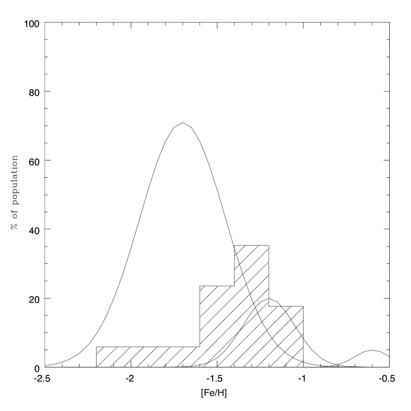
Figure 6: Histograms of [Fe/H] for the sample of 17 Kapteyn group stars, 15 of which may be kinematically related to $\omega$ Cen. The three gaussian curves represent the three suggested populations of $\omega$ Centauri at [Fe/H]=-1.7, -1.2 and -0.6, with the percentage of stars observed at that metallicity shown as 70%, 20% and 5% respectively (Norris et al. 1996)

Figure 6 shows a histogram of the [Fe/H] values of all 16 of the Kapteyn group stars. Also shown are the three suggested sub-populations of $\omega$ Centauri at [Fe/H] = -1.7, -1.2 and -0.5 (Norris & Da Costa, 1995). The metallicity distribution of the stars in the Kapteyn group falls towards the upper end of the extended MDF for the $\omega$ Cen stars. but is consistent with the cluster MDF. Abundances obtained for Na, Mg, Ca, Cu, Zr and Ba and their uncertainties are given in Table 7. The errors quoted are either the spread in derived abundances from different lines, or set to a standard value of 0.1 dex, representing the uncertainty in any individual measurement, whichever is the larger.

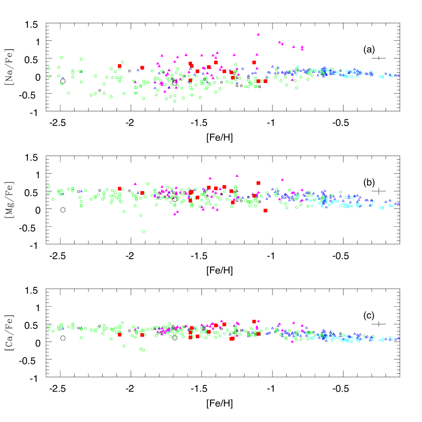
Figure 7: Plots of a) Na abundance, b) Mg abundance and c) Ca abundance. The red filled squares are those stars that may be kinematically linked to $\omega$ Cen, while the open black circles are those that do not appear to have kinematics link to the globular cluster. The small open black squares are stars from the Gratton peak (see Figure 1). Also shown are stars from the thin disk (small open cyan squares), thick disk (small open blue triangles) and halo (small open green circles) from Venn et al. 2004; stars from $\omega$ Cen (small filled magenta triangles) from Norris 1995 and Smith 2000. Typical error bars are shown in the top right of each plot.

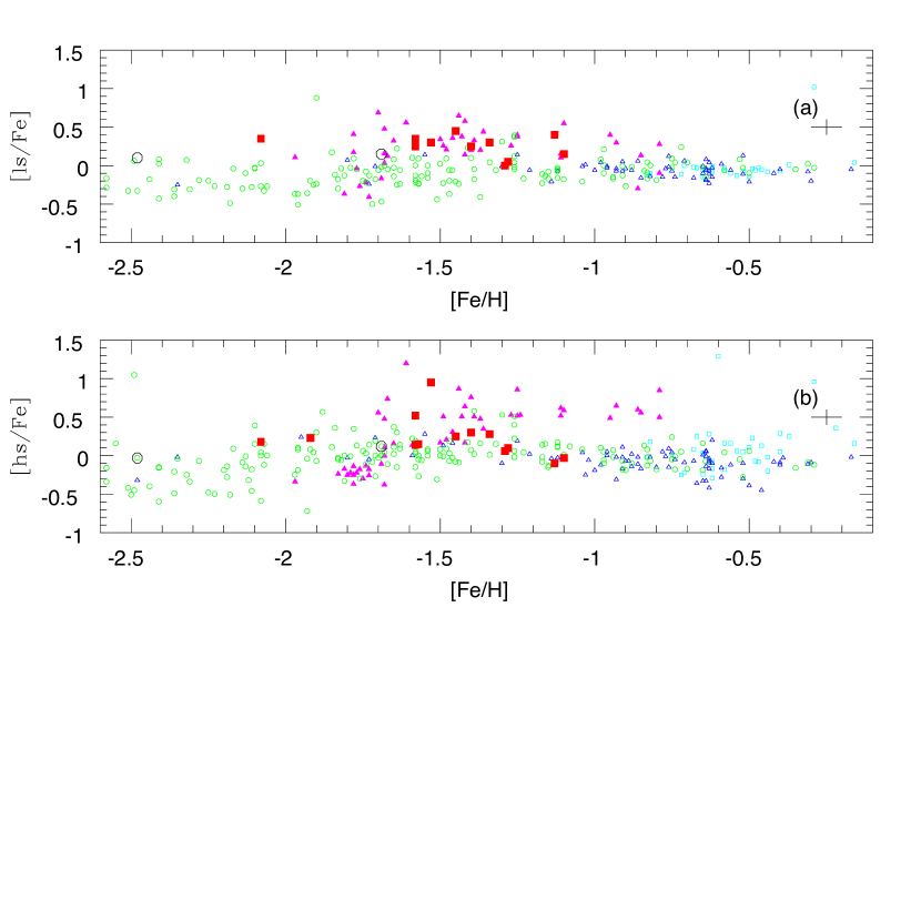
Figure 8: Plots of a) light s-process element abundances and b) heavy s-process element abundances. Symbols are the same as in Figure 7. The elements plotted in a) are Zr for the Kapteyn group and $\omega$ Cen stars and Y for the thin disk, thick disk and halo stars. The heavy s-process element plotted in b) is Ba for all samples. Typical error bars are shown in the top right of each plot.

Figure 7 shows the abundances for Na, Mg and Ca while Figure 8 shows the abundances for the light and heavy s-process elements. In both figures the red filled squares are those stars that are likely to be kinematically linked to $\omega$ Cen, while the black open circles are those that are probably not kinematically associated with the cluster. Also shown are stars from Venn et al. (2004) for the thin disk (cyan open squares), thick disk (blue open triangles) and halo (green open circles). Stars in $\omega$ Cen itself, from studies by Norris & Da Costa (1995) and Smith et al. (2000) are shown as magenta filled triangles. The Gratton peak stars are shown as small open black squares.

First we compare the abundances in $\omega$ Cen and in the field halo stars. Then we compare the Kapteyn group abundances with those in the cluster and the field halo, in order to ascertain whether the Kapteyn group stars show the abundance patterns of either of these two populations. The Na abundance in Figure 7a show a clear separation between the $\omega$ Cen studies (magenta filled triangles) and the halo stars (green open circles), although this distinction is not so clear for Mg. For Ca, there is separation in the more metal-rich regime ([Fe/H]$>-1.5$) with the distinction becoming less for more metal-poor stars. In Figure 8a the light s-process elements show show a marked difference between the abundances observed in $\omega$ Cen and the field halo stars, with $\omega$ Cen showing a strong relative enhancement in the light s-process elements. In Figure 8b, an even larger difference in Ba abundance is evident, with $\omega$ Cen showing a spread in Ba abundance from [Ba/Fe]=+1.0 to -0.4 over a range of metallicities . Again, as for Ca, this distinction becomes less at [Fe/H] near -1.7, where the separation is less and the two populations appear to overlap more. From these two figures it seems clear that there is a distinct difference between the Kapteyn stars believed to be kinematically related to $\omega$ Cen (red filled squares) and those that appear to be prograde field stars (black open circles). The prograde members of the Kapteyn sample show abundances that are consistent with being part of either the thick disk or halo populations.

The main point of interest here is that the Kapteyn stars which appear to be kinematically related to $\omega$ Cen in Figure 3 (red filled squares) share distinct abundance similarities with those stars from previous $\omega$ Cen studies (magenta filled triangles). The abundances for the potential $\omega$ Cen candidates among the Kapteyn stars could be drawn from the same abundance distribution as the $\omega$ Cen stars, although we note that there is much more scatter in the abundance distributions for most elements in the $\omega$ Cen stars. This larger scatter may be several causes: difference in the two studies making up this sample (Norris & Da Costa (1995) and Smith et al. (2000)); a genuine scatter in the abundances observed in $\omega$ Cen stars; or a combination of a genuine scatter and observational uncertainties. Whatever the reason for this large scatter in the cluster star abundances, it seems clear that the Kapteyn candidates show abundance anomalies relative to the field halo which are similar to those shown by the stars of $\omega$ Cen. The similarities between the Kapteyn candidates and the $\omega$ Cen stars, relative to the field halo, are clearest in Na, Mg and the s-elements.

Although the copper abundance was derived for only five of the stars in our sample, the results are worth mentioning. $\omega$ Cen is known for its unique copper signature. At a constant value of [Cu/Fe] $\sim-0.6$, it is distinct from the halo stars in the same metallicity range, which show an increase with metallicity up to [Cu/Fe] = -0.3 as discussed by Smith et al. (2000). Of the four stars for which copper was measured in our sample, all show deficiencies, with [Cu/Fe] values between -0.47 and -0.60. This adds weight to the case that this group of stars come from the same population as $\omega$ Cen. Copper was also detected in a fifth star, CD -30.1121, which is not believed to be kinematically linked to $\omega$ Cen. The copper value in this star was found to be [Cu/Fe] = -0.7. Copper has been seen to decrease sharply with metallicity among field halo stars, as shown in Sneden et al. (1991). With a metallicity of [Fe/H] = -1.69, the copper value seen in CD -30.1121 is consistent with the field halo star trend seen in copper and the observed low copper does not necessarily exclude it as a field halo star, as the kinematics suggest.

4.3 Statistical Analysis

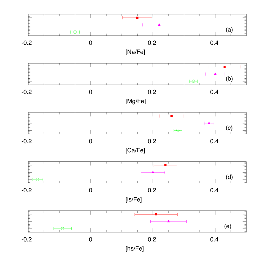
Figure 9: The mean abundance and standard deviation of the mean abundance of the Kapteyn group stars (filled red squares), $\omega$ Cen stars (filled magenta triangles)and halo stars (open green circles) for the five different elements studied: a) [Na/Fe], b) [Mg/Fe], c) [Ca/Fe], d) [ls/Fe] and e) [hs/Fe]. It is easy to see the mean abundance and distributions of each population and compare to the others. The y axis simply spreads the three different groups out for clarity and ease of comparison.

Statistical tests were undertaken on the abundance distributions to determine the likelihood that the three groups of stars (Kapteyn group, $\omega$ Cen and the halo) come from the same population. The $\omega$ Cen group consisted of stars from the Norris & Da Costa (1995) and Smith et al. (2000) studies and includes the stars from Gratton et al. (2003) only for elements in common with this study, Na, Mg and Ca. The halo group is taken from the Venn et al. (2004) compilation and is defined as being any halo population star that falls within the plausible range of [Fe/H] values for $\omega$ Cen as seen in Figure 6, that is [Fe/H] = -0.5 to -2.5. However, for completion, halo stars outside these values, while not included in the statistical analysis, are included in the abundance plots. Table 9 shows the mean, standard deviation $\sigma$ and standard deviation of the mean $\sigma_{mean}$, as defined by $\sigma_{mean}$=$\sigma$/$\sqrt{N}$ where N is the number of stars in each sample, also given in Table 9. Figure 9 shows this information graphically for the five elements studied, with the Kapteyn group again shown as filled red squares, the $\omega$ Cen stars as filled magenta triangles and the field halo stars as open green circles. It is evident from this figure that in all elements, except Ca and to a lesser extent Mg, the field halo stars are chemically distinct from $\omega$ Cen. It is also clear that, except for Ca, the Kapteyn group and $\omega$ Cen populations overlap in [X/Fe].

It should be noted that results from a very recent study of 66 red giant stars in $\omega$ Cen by Johnson et al. (2009) strongly supports these results. They find a general increase in [Na/Fe] with increasing metallicity, from $<$[Na/Fe]$>$=+0.03 ($\sigma$=0.32) at the lower metallicity end to $<$[Na/Fe]$>$=+0.86 ($\sigma$=0.12) for higher metallicity. They also find $<$[Ca/Fe]$>$=+0.36 ($\sigma$=0.09), La values varying from [La/Fe]=-0.4 to +2.0 and $<$[Eu/Fe]$>$=+0.19 ($\sigma$=0.23). These results strongly overlap with the previous studies of $\omega$ Cen stars used as a comparison with the Kapteyn group stars in this study.

A parametric t-test and a non-parametric Kolmogorov-Smirnov test were performed on the abundance distributions. The results are shown in Tables 10 and 11 respectively. In these tests, a small P value means that the two populations are distinct. We adopted the standard criterion that P$<0.05$ is needed to reject the null hypothesis. The tables show that both the parametric and non-parametric test gave the same results. Tests in which the P value satisfied the requirement are shown in bold, indicating that the two populations compared are statistically different. $\omega$ Cen and the halo were seen to be distinct separate populations in all of the five element distributions, in both tests. The Kapteyn group and the halo were statistically different in [Na/Fe], [ls/Fe] and [hs/Fe] while the [Mg/Fe] and [Ca/Fe] comparison is inconclusive. The Kapteyn group and $\omega$ Cen differ only in [Ca/Fe]. While the [hs/Fe] abundance patterns seen in Kapteyn and $\omega$ Cen in Figure 8b differ slightly, there is enough overlap in the two groups for this overlap to be statistically significant and the statistical analysis suggests these two distributions can come from the same population. There appear to be only two Ba enhanced stars in the Kapteyn group sample, although both are seen at values consistent with Ba enhancements seen in $\omega$ Cen stars. The apparent lack of Ba enhanced stars in the Kapteyn group may be due to a small sample size of only 16 stars.

Together with Figures 7 and 9, these statistical tests show that [Ca/Fe] does not differ enough between the populations to give reliable discrimination. The [Ca/Fe] relationship in Figure 7 is tight and all populations overlap. However, the difference seen in the remaining four elements provide enough information to show that the field halo stars are different from both the Kapteyn stars and the $\omega$ Cen stars and that the Kapteyn group stars are chemically similar to those in $\omega$ Cen.

5 Discussion and Conclusion

The kinematic and abundance analysis in this study suggests that at least our 14 members of the Kapteyn group and potentially many more stars in retrograde orbits which were not observed in this study, could be remnants of tidal debris stripped from the parent galaxy of $\omega$ Cen, or even from the cluster itself, during its merger with the Galaxy.

Our study provides the first detailed chemical evidence of field stars that appear to be both kinematically and chemically related to $\omega$ Cen. It may lend weight to the view that $\omega$ Cen is the remnant nucleus of a disrupted dwarf galaxy which was accreted by the Milky Way, by providing chemical evidence of tidal debris among the Galactic field stars.

The three-banded structure seen in the Lindblad diagrams of Figures 3 and described in Section 2.1 may be indicative of stars shed with different energies from different wraps of the decaying orbit of the parent galaxy around the Milky Way. The reader is referred to Figure 6 in Meza et al. (2005) which shows several distinct E–L_z curves from their numerical simulations of merger debris. In this study there is currently no evidence for an abundance difference between stars of different wraps of the orbit. A study involving higher quality data and a larger number of stars from these wraps is underway. The presence of this banded structure, along with the present Galactic radius of $\omega$ Cen, suggest the original parent galaxy was relatively massive in order for dynamical friction to have the required effect, and was also relatively dense in order to survive the Galactic tidal stresses in to the current orbital radius of $\omega$ Cen.

What else can we infer about the parent galaxy? If our stars are debris from the parent galaxy, then the galactic metallicity-luminosity relationship and the mean metallicity of the sample ($\langle{\rm[Fe/H]}\rangle=-1.5$) indicate that the parent galaxy’s luminosity would have been about $M_{V}\sim-11$. Its luminosity would have been about $2\times 10^{6}$ L_⊙, and its stellar mass $\sim 4\times 10^{6}$ M_⊙. This stellar mass is comparable to the present stellar mass of $\omega$ Cen itself. The total mass of the parent galaxy could have been as high as $5\times 10^{8}$ M_⊙ if it were a dwarf galaxy with a dark matter content similar to the Fornax dSph (e.g Walker et al. (2006)).

What are the chances of finding $\omega$ Cen debris stars in the solar neighborhood from such a low-mass galaxy? We can use the Meza et al. simulation as a guide, although a detailed comparison is not appropriate as these authors note, because their end-product galaxy is not like the Milky Way. In summary, the debris of their satellite is well mixed azimuthally by redshift 0.48, at least within 10 kpc radius from the center of their parent galaxy, and is confined to a disk-like layer. The satellite is disrupted in its last three perigalactic passages, leaving a significant amount of substructure in E and L_z. We focus on the lowest $L_{z}$ substructure in their simulation, as a qualitative counterpart to the proposed $\omega$ Cen debris. Most of our stars lie in a volume of radius $\sim 500$ pc around the sun, and in a broad range of retrograde L_z. For comparison, we can estimate the fraction of the Meza et al. debris which would lie within our $500$ pc volume and within their lowest L_z substructure: it is about $1.5\times 10^{-4}$. We could therefore expect to find about 700 debris stars in our volume and within the lowest angular momentum substructure, if we use the Meza et al. simulations as a guide and assume that the typical star in this population has a mass of about 0.8 M_⊙. In the Dinescu region shown in Figure 3, we have compiled a total of about 100 stars. Even if all of them turn out to be $\omega$ Cen debris stars, then this comparison may indicate that there are plenty more $\omega$ Cen debris stars to be found nearby.

We should also consider the possibility that the Kapteyn group stars were stripped from the cluster itself as its outer regions were disrupted by the Galactic tidal field. This would be the immediate inference from the the chemical similarity which we have demonstrated between the Kapteyn group stars and Cen stars. This seems unlikely, because the in-spiralling time under the influence of dynamical friction is in excess of the Hubble time for a cluster with the mass of $\omega$ Cen; also, we note that the Kapteyn group stars are significantly more energetic than the cluster itself. It seems likely that the group stars came from the body of the parent dwarf galaxy, and therefore that the chemical peculiarities of $\omega$ Cen are shared by its parent, and may well have originated in gas which was funneled into the cluster, possibly over an extended period, as suggested by Norris et al. (1997). Detailed numerical models of the chemical and dynamical evolution of $\omega$ Cen as its galaxy loses mass in the Galactic tidal field are needed.

Acknowlegements ECW is funded by Australian Research Council grant DP0772283. KCF acknowledges his late colleagues Olin Eggen and Alex Rodgers for their work on the Kapteyn’s star group which prompted this paper. We would also like to add our thanks to the referee (D. Casetti-Dinescu) for many helpful comments and suggestions.. We thank Mike Bessell for his major improvements to the echelle spectrograph which made this work possible; Daniela Carollo for discussions which led to the association of the Kapteyn’s star group with $\omega$ Cen and for comments on an earlier draft of this paper; John Norris and Tim Beers for discussions and encouragement; and the SSO staff for maintaining the SSO instrumentation.

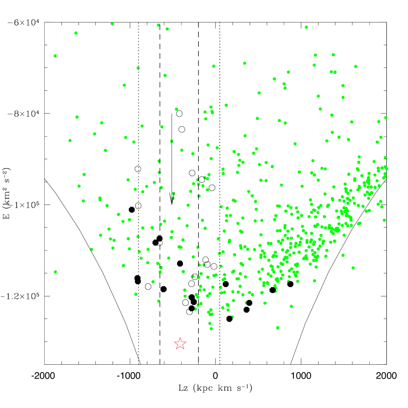
Figure 3: Lindblad diagram for Kapteyn group. The black filled circles are the 16 Kapteyn values, as shown in Table 2, and the red star indicates the position of $\omega$ Centauri. The black open circles are stars from the Gratton $\omega$ Cen peak, as seen in Figure 1, with a filter of L_z = -1000 to 0 kpc km s^-1. The small green filled circles are stars from the Beers et al. 2000 catalogue with a filter of [Fe/H] = -2.5 to -0.5, the accepted range observed in $\omega$ Centauri. The box outlined by the dashed lines shows the zone in which stars are considered to be candidates from $\omega$ Cen’s host galaxy, as defined by Dinescu (2002). The smaller dotted lines show this same region when taking into account uncertainties on the values of the Local Standard of Rest (for more detail, see text). The arrow indicating L${}_{z}=-510$ kpc km s^-1 shows the L_z value for Kapteyn’s star itself, using the original values from Eggen (1996). The solid curves represent the circular orbit loci for this potential.

Figure 5: Comparison of a) photometric and spectroscopic temperatures and b) photometric and spectroscopic gravities. In each plot, the one-to-one relation is overplotted.

Table 1: Kinematics for the Kapteyn group of stars.

Star	RA	DEC	$\mu_{\alpha}$	$\mu_{\delta}$	$V$${}_{\textrm{rad}}$	Distance
	∘	∘	m′′ yr-1	m′′ yr-1	km s-1	pc
HD 13979	33.84	-25.92	29.78	-47.67	54.0	453
HD 21022	50.59	-32.99	31.13	-32.51	110.0	1115
HD 110621	190.93	-44.68	-221.96	-17.30	219.0	156
HD 111721	192.86	-13.49	-273.70	-321.99	27.0	162
HD 181007	289.87	-20.43	-39.97	-170.25	-2.0	396
HD 181743	290.93	-45.08	-70.60	-814.46	26.0	92
HD 186478	296.31	-17.49	-22.23	-84.42	31.0	1017
HD 188031	298.74	-42.65	2.87	-436.00	-139.0	163
HD 193242	304.98	-19.91	-20.64	-97.64	-128.0	314
HD 208069	328.61	-30.26	132.14	-198.67	-167.0	285
HD 215601	341.70	-31.87	56.11	-148.35	-35.0	278
HD 215801	342.12	-46.06	33.49	-305.71	-86.0	159
BD -13 3834	212.61	-13.93	-337.04	-458.34	126.0	…
CD -30 1121	44.25	-30.41	31.11	-28.51	104.0	629
CD -62 1346	316.51	-61.56	-14.97	-102.19	127.0	299
G 18-54	337.90	2.16	51.69	-328.64	-210.4	178
G 24-3	301.43	4.05	-133.27	-171.24	-208.9	175

Table 2: Space motions, angular momentum and energies for Kapteyn stars. The $\sigma$ values quoted are those derived from a Monte Carlo simulation (see text for details).

Star	$U$	$\sigma_{U}$	$V$	$\sigma_{V}$	$W$	$\sigma_{W}$	$L_{z}$	$E$
	km s-1		km s-1		km s-1		kpc km s-1	105 km2s-2
HD 13979	-18	5	-115	24	-28	3	874	-1.17
HD 21022	-24	11	-249	44	5	19	-278	-1.20
HD 110621	19	30	-255	20	58	5	-280	-1.23
HD 111721	57	15	-273	55	-135	33	-415	-1.13
HD 181007	-89	19	-301	63	-51	12	-608	-1.18
HD 181743	42	14	-335	70	-56	11	-913	-1.16
HD 186478	-177	29	-368	79	-62	13	-979	-1.01
HD 188031	162	11	-309	66	16	12	-701	-1.08
HD 193242	45	13	-172	28	47	7	363	-1.23
HD 208069	172	17	-302	57	7	27	-654	-1.07
HD 215601	12	5	-198	42	7	11	162	-1.25
HD 215801	14	6	-204	46	123	12	118	-1.17
CD -30 1121	15	4	-141	24	-43	9	667	-1.19
CD -62 1346	-73	8	-167	28	-27	11	394	-1.21
G 18-54	-55	20	-335	42	1	31	-908	-1.17
G 24-3	2	26	-252	24	85	5	-254	-1.21

Table 3: Constants used in Galactic potential calculations.

Region	Values
Bulge	Mb = 1.12 x 1010M⊙
	ab= 0.0 kpc
	bb = 0.277 kpc
Disk	Md = 8.07 x 1010M⊙
	ad= 3.7 kpc
	bd = 0.20 kpc
Dark Halo	Mh = 5 x 1010M⊙
	d = 6.0 kpc
	$\Phi_{\textrm{offset}}$ = -12.3 x 104

Table 4: Kinematic values of $\omega$ Centauri.

$\omega$ Centauri	Parameters
RA	201.44∘
DEC	-47.00∘
$\mu_{\alpha}$	-5.08 m′′ yr-1
$\mu_{\delta}$	-3.57 m′′ yr-1
$V$${}_{\textrm{rad}}$	232.5 km s-1
Distance	4900 pc
$U$	-61 km s-1
$V$	-36 km s-1
$W$	6 km s-1
$L_{z}$	-413 kpc km s-1
Energy	-1.30 x 105 km2s-2

Table 5: Atmospheric parameters adopted for individual stars

Star	V	T${}_{\textrm{eff}}$	log g	$\chi$	[Fe/H]
		($\pm$ 150K)	$\pm$ 0.20	$\pm$0.25km s-1
HD 13979	9.16	5050	2.25	2.35	-2.48
HD 21022	9.19	4550	1.25	1.85	-2.08
HD 110621	9.85	5850	3.80	0.90	-1.41
HD 111721	7.85	5000	2.60	1.52	-1.34
HD 181007	9.24	5000	2.60	1.30	-1.58
HD 181743	9.65	6050	3.35	1.00	-1.47
HD 186478	8.85	5000	1.80	1.90	-1.92
HD 188031	10.06	6400	3.75	0.95	-1.13
HD 193242	9.10	5150	2.75	1.38	-1.58
HD 208069	9.20	5250	2.25	1.80	-1.57
HD 215601	8.39	5110	1.80	1.75	-1.10
HD 215801	9.99	6470	3.75	0.50	-1.12
CD -30 1121	10.30	4960	2.45	1.00	-1.63
CD -62 1346	9.84	5150	1.95	1.90	-1.39
G 18-54	10.66	6150	4.25	1.05	-1.28
G 24-3	10.44	6550	4.00	1.60	-1.29

Table 6: Line list used to obtain abundances via spectrum synthesis.

Species	Wavelength	log gf	$\chi$
	Å		eV
Na I	5889.95	0.00	0.117
	5895.92	0.00	-0.184
Mg I	5183.60	2.72	-0.180
	5528.41	4.34	-0.620
	5711.09	4.34	-1.833
Ca I	6122.22	1.88	-0.409
	6162.17	1.90	0.100
	6439.08	2.52	0.470
	6490.84	5.80	-4.745
Cu I	5105.55	1.39	-1.516
	5782.03	1.64	-3.432
Zr II	4208.98	0.713	-0.460
Ba II	5853.68	0.60	-1.010
	6141.72	0.704	-0.503
	6496.90	0.604	-0.380

Table 7: Average element abundances of Na, Mg, Ca, Cu, Zr and Ba for all stars in the sample.

Star	[Fe/H]	[Na/Fe]	$\sigma$	[Mg/Fe]	$\sigma$	[Ca/Fe]	$\sigma$	[Cu/Fe]	$\sigma$	[Zr/Fe]	$\sigma$	[Ba/Fe]	$\sigma$
HD 21022	-2.08	0.28	0.11	0.57	0.12	0.20	0.17	…	…	0.35	0.15	0.18	0.25
HD 110621	-1.40	0.38	0.10	0.58	0.10	0.46	0.24	…	…	0.25	0.15	0.30	0.14
HD 111721	-1.34	0.13	0.10	0.62	0.10	0.49	0.13	-0.47	0.39	0.30	0.15	0.28	0.14
HD 181007	-1.58	0.35	0.10	0.45	0.10	0.26	0.24	-0.60	0.14	0.35	0.15	0.52	0.10
HD 181743	-1.45	0.25	0.10	0.60	0.29	0.28	0.17	…	…	0.45	0.15	0.25	0.10
HD 186478	-1.92	0.23	0.18	0.45	0.10	0.19	0.10	…	…	…	…	0.23	0.10
HD 188031	-1.36	0.38	0.10	0.37	0.29	0.57	0.10	…	…	0.40	0.15	-0.10	0.10
HD 193242	-1.58	-0.13	0.10	0.23	0.31	0.12	0.25	…	…	0.25	0.15	0.14	0.10
HD 208069	-1.57	0.28	0.10	0.48	0.33	0.39	0.16	…	…	…	…	0.15	0.10
HD 215601	-1.10	-0.15	0.10	0.73	0.10	0.22	0.10	-0.60	0.10	0.15	0.15	-0.03	0.25
HD 215801	-1.05	-0.15	0.10	-0.05	0.35	…	…	…	…	…	…	…	…
CD -62.1346	-1.53	0.13	0.10	0.32	0.10	0.15	0.10	-0.55	0.10	0.30	0.15	0.95	0.10
G 18-54	-1.28	-0.05	0.10	0.18	0.10	0.09	0.10	…	…	0.05	0.15	0.19	0.10
G 24-3	-1.29	0.10	0.10	0.50	0.10	0.08	0.18	…	…	0.00	0.15	0.06	0.10
HD 13979	-2.48	-0.15	0.10	-0.03	0.39	0.10	0.14	…	…	0.10	0.15	-0.03	0.10
CD -30.1121	-1.69	-0.20	0.14	0.27	0.21	0.11	0.10	-0.70	0.10	0.15	0.15	0.12	0.10

Table 8: Sensitivity of derived log $\epsilon$ abundances to chosen atmospheric parameters

Species	$\Delta$ T${}_{\textrm{eff}}$	$\Delta$ log g	$\Delta$ $\chi$
	(-200K)	(-0.30)	(-0.30 km s-1)
Na I	-0.20	+0.07	-0.12
Mg I	-0.13	+0.03	-0.06
Ca I	-0.13	+0.03	-0.17
Cu I	-0.19	0.00	0.00
Zr II	-0.09	-0.09	-0.17
Ba II	-0.15	-0.08	-0.28

Table 9: Mean values, standard deviations and standard deviations of the means for all abundance arrays.

Species	Kap	Omega	Halo
	(N=14)	(N=50)	(N=275)
$<[$Na/Fe$]>$	0.15	0.22	-0.07
$\sigma$	0.18	0.38	0.23
$\sigma_{mean}$	0.050	0.054	0.014
$<[$Mg/Fe$]>$	0.43	0.40	0.33
$\sigma$	0.19	0.22	0.21
$\sigma_{mean}$	0.050	0.056	0.013
$<[$Ca/Fe$]>$	0.26	0.38	0.28
$\sigma$	0.15	0.11	0.16
$\sigma_{mean}$	0.041	0.015	0.010
$<[$ls/Fe$]>$	0.24	0.20	-0.17
$\sigma$	0.14	0.27	0.27
$\sigma_{mean}$	0.038	0.038	0.016
$<[$hs/Fe$]>$	0.21	0.25	-0.09
$\sigma$	0.26	0.41	0.48
$\sigma_{mean}$	0.070	0.058	0.029

Table 10: The results of a parametric t-test on the means and standard deviations of the different populations from the Kapteyn group, the halo stars and previous Omega Cen studies. If the p-value is $``$small” (i.e. p$<$ 0.05) then the two groups are considered to be from different populations. If p is larger than 0.05, the test is inconclusive. Those values shown in bold are the stellar groups that statistically appear to come from different populations.

Species		Kap : Halo	Kap : Omega	Omega : Halo
$[$Na/Fe$]$	t	3.078	0.985	3.796
	p	0.003	0.332	0.000
$[$Mg/Fe$]$	t	1.965	0.516	2.063
	p	0.069	0.612	0.044
$[$Ca/Fe$]$	t	0.483	2.791	5.366
	p	0.645	0.013	0.000
$[$ls/Fe$]$	t	9.096	0.689	8.009
	p	0.000	0.495	0.000
$[$hs/Fe$]$	t	3.933	0.442	5.155
	p	0.000	0.662	0.000

Table 11: The results of a non-parametric Kolmogorov-Smirnov test on the different populations from the Kapteyn group, the halo stars and previous Omega Cen studies. If P is $``$small” (i.e. P $<$ 0.05) then the two groups are considered to be from different populations. If P is larger than 0.05, the test is inconclusive. As for Table 10, those values shown in bold are the stellar groups that statistically appear to come from different populations.

Species		Kap : Halo	Kap : Omega	Omega : Halo
$[$Na/Fe$]$	D	0.5304	0.3200	0.4212
	P	0.000	0.152	0.000
$[$Mg/Fe$]$	D	0.3220	0.1933	0.2255
	P	0.084	0.734	0.020
$[$Ca/Fe$]$	D	0.2504	0.5543	0.3585
	P	0.329	0.001	0.000
$[$ls/Fe$]$	D	0.7814	0.1905	0.6307
	P	0.000	0.849	0.000
$[$hs/Fe$]$	D	0.4166	0.3771	0.4299
	P	0.010	0.066	0.000

References

- Alonso et al. (1996) Alonso, A., Arribas, S., & Martinez-Roger, C. 1996, A&A, 313, 873
- Alonso et al. (1999) Alonso, A., Arribas, S., & Martínez-Roger, C. 1999, A&AS, 140, 261
- Anders & Grevesse (1989) Anders, E., & Grevesse, N. 1989, Geochim. Cosmochim. Acta, 53, 197
- Beers et al. (2000) Beers, T. C., Chiba, M., Yoshii, Y., Platais, I., Hanson, R. B., Fuchs, B., & Rossi, S. 2000, AJ, 119, 2866
- Bekki & Freeman (2003) Bekki, K., & Freeman, K. C. 2003, MNRAS, 346, L11
- Burris et al. (2000) Burris, D. L., Pilachowski, C. A., Armandroff, T. E., Sneden, C., Cowan, J. J., & Roe, H. 2000, ApJ, 544, 302
- De Silva et al. (2007) De Silva, G. M., Freeman, K. C., Bland-Hawthorn, J., Asplund, M., & Bessell, M. S. 2007, AJ, 133, 694
- Dehnen (1998) Dehnen, W. 1998, AJ, 115, 2384
- Dettbarn et al. (2007) Dettbarn, C., Fuchs, B., Flynn, C., & Williams, M. 2007, A&A, 474, 857
- Dinescu (2002) Dinescu, D. I. 2002, in Astronomical Society of the Pacific Conference Series, Vol. 265, Omega Centauri, A Unique Window into Astrophysics, ed. F. van Leeuwen, J. D. Hughes, & G. Piotto, 365–+
- Dinescu et al. (1999) Dinescu, D. I., Girard, T. M., & van Altena, W. F. 1999, AJ, 117, 1792
- Eggen (1996) Eggen, O. J. 1996, AJ, 112, 1595
- Eggen et al. (1962) Eggen, O. J., Lynden-Bell, D., & Sandage, A. R. 1962, ApJ, 136, 748
- Freeman & Bland-Hawthorn (2002) Freeman, K., & Bland-Hawthorn, J. 2002, ARA&A, 40, 487
- Fulbright (2000) Fulbright, J. P. 2000, AJ, 120, 1841
- Gratton et al. (2003) Gratton, R. G., Carretta, E., Desidera, S., Lucatello, S., Mazzei, P., & Barbieri, M. 2003, A&A, 406, 131
- Johnson et al. (2009) Johnson, C. I., Pilachowski, C. A., Michael Rich, R., & Fulbright, J. P. 2009, ApJ, 698, 2048
- Klement et al. (2009) Klement, R. et al. 2009, ApJ, 698, 865
- Meza et al. (2005) Meza, A., Navarro, J. F., Abadi, M. G., & Steinmetz, M. 2005, MNRAS, 359, 93
- Miyamoto & Nagai (1975) Miyamoto, M., & Nagai, R. 1975, PASJ, 27, 533
- Mizutani et al. (2003) Mizutani, A., Chiba, M., & Sakamoto, T. 2003, ApJ, 589, L89
- Morrison et al. (2009) Morrison, H. L. et al. 2009, ApJ, 694, 130
- Navarro et al. (2004) Navarro, J. F., Helmi, A., & Freeman, K. C. 2004, ApJ, 601, L43
- Norris et al. (1997) Norris, J. E., Freeman, K. C., Mayor, M., & Seitzer, P. 1997, ApJ, 487, L187
- Norris & Da Costa (1995) Norris, J. E., & Da Costa, G. S. 1995, ApJ, 447, 680
- Olling & Merrifield (2000) Olling, R. P., & Merrifield, M. R. 2000, MNRAS, 311, 361
- Paczynski (1990) Paczynski, B. 1990, ApJ, 348, 485
- Reid et al. (2009) Reid, M. J., Menten, K. M., Zheng, X. W., Brunthaler, A., Moscadelli, L., Xu, Y., Zhang, B., Sato, M., Honma, M., Hirota, T., Hachisuka, K., Choi, Y. K., Moellenbrock, G. A., & Bartkiewicz, A., 2009, ApJ, 700, 137
- Searle & Zinn (1978) Searle, L., & Zinn, R. 1978, ApJ, 225, 357
- Smith et al. (2000) Smith, V. V., Suntzeff, N. B., Cunha, K., Gallino, R., Busso, M., Lambert, D. L., & Straniero, O. 2000, AJ, 119, 1239
- Sneden et al. (1991) Sneden, C. A., Gratton, R. G., & Crocker, D. A. 1991, A&A, 246, 354
- Sneden (1973) Sneden, C. A. 1973, PhD thesis, The University of Texas at Austin
- Venn et al. (2004) Venn, K. A., Irwin, M., Shetrone, M. D., Tout, C. A., Hill, V., & Tolstoy, E. 2004, AJ, 128, 1177
- Walker et al. (2006) Walker, M. G., Mateo, M., Olszewski, E. W., Bernstein, R., Wang, X., & Woodroofe, M. 2006, AJ, 131, 2114