Gluon Saturation Effects at the Nuclear Surface: Inelastic Cross Section of Proton-Nucleus in the Ultra High Energy Cosmic Ray domain

Abstract

Considering the high-energy limit of the QCD gluon distribution inside a nucleus, we calculate the proton-nucleus total inelastic cross section using a simplified dipole model. We show that, if gluon saturation occurs in the nuclear surface region, the total cross section of proton-nucleus collisions increases more rapidly as a function of the incident energy compared to that of a Glauber-type estimate. We discuss the implications of this with respect to recent ultra-high-energy cosmic ray experiments.

1 Introduction

In the ultra-high-energy domain, the mechanism of inelastic hadronic collisions is dominated by the contribution from small-$x$ gluons. This is the basic reason why the total or inelastic proton-proton collision cross section increases as a function of the incident energy. A simple way to see this is to use the eikonal expression for the reaction cross section in the impact parameter representation as

$$\sigma_{r}=\int d^{2}\mathbf{b}[1-\exp(-2\chi(\mathbf{b},s))],$$ (1)

where the eikonal $\chi(\mathbf{b},s)$ counts essentially the total number of possible scattering centers of the constituents inside the target “seen” by the projectile passing through the target along a straight line with the impact parameter $\mathbf{b,}$ and with center-of-mass energy $\sqrt{s}$.

If the target is thick enough, the eikonal function is much larger than unity ( $\chi(\mathbf{b},s)\gg 1$) in the central region, but it falls down to zero in the surface region. The integrand of Eq.(1) keeps a value almost equal to unity while $\chi(\mathbf{b},s)\gg 1,$ and falls down quickly to zero near the surface. From this we may determine an effective radius $b_{1/2}$ such that the integral (1) is approximately given by

$$\sigma_{r}\simeq\pi b_{1/2}^{2}.$$ (2)

Here $b_{1/2}$ might be estimated by fixing the value of $\chi(\mathbf{b}_{1/2},s)$, for example, as

$$\chi(\mathbf{b}_{1/2},s)=\ln 2,$$ (3)

so that the effective radius depends on the energy $b_{1/2}=b_{1/2}\left(\sqrt{s}\right)$. Let us assume that the eikonal function factorizes in the form

$$\chi(\mathbf{b},s)=P(\mathbf{b})N(\sqrt{s}),$$ (4)

where $P(\mathbf{b})$ is the probability distribution of the scattering center (e.g., partons) in the transverse plane and $N(x)$ is the number of partons which can interact for a given $\sqrt{s}$. Suppose that $P(\mathbf{b})$ is a two-dimensional Gaussian distribution of width $R,$

$$P(\mathbf{b})=\frac{1}{\left(\pi R\right)^{2}}e^{-\frac{b^{2}}{R^{2}}}$$ (5)

and that, for large $\sqrt{s}$, the number of partons increase with $\sqrt{s}$ as

$$N(x)\propto\sqrt{s}^{\alpha}.$$ (6)

Then, we have

$$b_{1/2}^{2}\left(\sqrt{s}\right)=\alpha R^{2}\ln\sqrt{s}+Const.$$ (7)

In such a situation, the reaction cross section increases as function of the incident energy for very large $\sqrt{s}$ as

$$\sigma_{r}\simeq\alpha\pi R^{2}\ln\sqrt{s}.$$ (8)

If the edge of the distribution has an exponential tail instead of a Gaussian distribution, a similar argument will show that the cross section would increase as

$$\sigma_{r}\simeq Const\times\left(\ln\sqrt{s}\right)^{2}.$$ (9)

The important point of this simple argument is that the rate of increase is related to the diffuseness $R$ of the probability distribution of the scattering center. The more diffuse the surface thickness is, the more quickly the reaction cross section increases as function of the incident energy. The possibility of such a mechanism, not only in the proton-proton but also in nucleus-nucleus cross section, was suggested many years ago [1, 2].

In this paper we explore the idea of [1, 2] in the language of the QCD gluon saturation mechanism for the proton-nucleus reaction. We show that, if the gluon distribution becomes saturated at some energy scale inside the nuclear surface region, then the reaction cross section of proton-nucleus collisions starts to increase very quickly and eventually overcomes the values estimated by the usual Glauber type of calculation.

Applying a simple effective dipole model for the reaction mechanism, we find that such an energy scale is of the order of $10^{17}-10^{18}eV.$ Above this energy scale, the behavior of the proton-nucleus cross section begins to change. We suggest that such an energy dependence of the proton-nucleus cross section may be observed in terms of the quantity called $\left\langle X_{\max}\right\rangle$ in the air showers of ultra-high-energy cosmic rays. Using a very simple toy model estimate of $\left\langle X_{\max}\right\rangle$, we show that our calculated values of the proton-nucleus reaction cross section are consistent with the recently observed $\left\langle X_{\max}\right\rangle$ by the Pierre Auger Observatory experiments [3] for incident protons at ultra-high energies.

2 Effective Dipole Model for the Proton-Proton Cross Section

To explore the above idea, we need the total cross section of proton-proton as function of incident energy which permit to extrapolate to the ultra-high energy region. For this purpose, we introduce an extremely simplified version of the dipole saturation model for the purpose of illustrating our idea here. The original dipole model was first introduced by Mueller [4] and extended to the impact parameter representation by Kowalski and Teaney [5]. Recently this model was applied to fit diffractive structure functions in electron-Nucleus collisions [6, 7, 8]. An application to proton-proton processes can be found in [9], where the incident proton is represented by dipoles associated with the valence quarks, having a probability distribution for different sizes specified by the proton wave function.

In this work, for simplicity, we assume that the proton is described by an effective dipole of a given size $R_{D}$, where we fix the dipole size $R_{D}$ by the average dipole radius

$$R_{D}^{2}=\int d^{2}r_{T}r_{T}^{2}|\Psi_{p}(r_{T})|^{2},$$

where $\Psi_{p}(r_{T})$ is the proton dipole wave function [10] in the transverse plane.

In this case, the gluon saturation model leads to a reaction cross section,

$$\sigma_{r}\left(\sqrt{s}\right)=2\pi\int_{0}^{\infty}bdb\ \left(1-e^{-2\chi}\right),$$ (10)

where the eikonal for the proton-proton reaction can be written as

$$\chi(\mathbf{b},s)=\frac{\pi^{2}}{N_{c}}R_{D}^{2}\alpha_{s}(Q^{2})xg(x,Q^{2})T_{p}(\mathbf{b}).$$ (11)

In this expression, the quantity $xg(x,Q^{2})$ is the parton distribution function (PDF), and represents the gluon density $x-$distribution in the target at a scale $Q^{2}$, and $\alpha_{s}(Q^{2})$ is the strong coupling defined at this scale. Following the steps of [8] we use

$$Q^{2}=\frac{C}{R_{D}^{2}}+Q_{0}^{2},$$ (12)

$$x=\frac{Q^{2}}{Q^{2}+s},$$ (13)

$$\alpha_{s}(Q^{2})=\frac{4\pi}{\left(11-\frac{2}{3}N_{f}\right)\log\left(\frac{Q^{2}}{\Lambda_{QCD}^{2}}\right)},$$ (14)

with $N_{f}=3$ and $\Lambda_{QCD}=0.192~{}GeV$.

For the profile function $T_{p}(\mathbf{b})$ of a proton, we consider the two different cases described in below.

2.1 Gaussian profile function

Suppose that the transverse probability distribution of gluons (profile function) inside the proton is of a Gaussian type:

$$T_{p}(\mathbf{b})=\frac{1}{\pi R_{p}^{2}}\exp{\left(\frac{-b^{2}}{R_{p}^{2}}\right).}$$ (15)

Writing Eq.(10) as

$$\sigma_{r}\left(\sqrt{s}\right)=2\pi R_{p}^{2}\int_{0}^{\infty}xdx\ \left(1-e^{-ae^{-x^{2}}}\right)$$ (16)

$$= \pi R_{p}^{2}\int_{0}^{1}\frac{du}{u}\ \left(1-e^{-au}\right)$$

$$= \pi R_{p}^{2}\left\{\gamma_{E}-ChI\left(a\right)+ShI(a)+\ln\left(a\right)\right\}$$

$$\equiv \pi R_{p}^{2}F(a),$$

where

$$a=\frac{\pi}{N_{c}}\frac{R_{D}^{2}}{R_{p}^{2}}\alpha_{s}(Q^{2})xg(x,Q^{2}),$$ (17)

$\gamma_{E}$ is the Euler constant, $ChI\left(a\right)$ and $ShI(a)$ are hyperbolic-cosine and hyperbolic-sine integral functions. The function

$$F(a)=\left\{\gamma_{E}-ChI\left(a\right)+ShI(a)+\ln\left(a\right)\right\}$$ (18)

is a monotonic increasing function of $a.$ From these expressions, we have $a\propto\sqrt{s}^{\alpha}$ and $F\left(a\right)\simeq\ln\left(a\right)$ for very large $\sqrt{s},$ so that the reaction cross section behaves at large incident energies as

$$\sigma_{r}\simeq\alpha\ \pi R_{p}^{2}\ln\left(\sqrt{s}\right)+Const.$$ (19)

as expected from the simple argument presented in the Introduction.

2.2 Profile function with exponential tail

Another important possibility is that the spatial gluon distribution has an exponential tail instead of a Gaussian, such as in a Woods-Saxon distribution. In this case, the asymptotic increase of the cross section as function of energy is expected as $\log^{2}\left(\sqrt{s}\right)$ and not $\log\left(\sqrt{s}\right),$ as discussed in the Introduction. However, since the Woods-Saxon distribution has 2 parameters (half-density radius $R_{1/2}$ and surface thickness $d$), we use the following profile function which has exponential tail, for simplicity.

$$T_{p}\left(\vec{b}\right)=\frac{1}{4\pi C_{T}\bar{R}_{p}^{2}}\frac{1}{\cosh\left(\frac{b}{\bar{R}_{p}}\right)},$$ (20)

where $C_{T}$ is the Catalan number,

$$C_{T}=\sum_{i=0}^{\infty}\frac{\left(-1\right)^{i}}{\left(2i+1\right)!}\simeq 0.9160.$$ (21)

The width parameter $\bar{R}_{p}$ is related to the mean-square of the impact parameter $\left\langle b^{2}\right\rangle$ as

$$\left\langle b^{2}\right\rangle=\nu\bar{R}_{p}^{2}.$$ (22)

and consequently to the radius parameter of the Gaussian case as $\bar{R}_{p}=\sqrt{\nu}R_{p},$ where

$$\nu=\frac{\int_{0}^{\infty}x^{3}/\cosh x\ dx}{\int_{0}^{\infty}x/\cosh x\ dx}\ \simeq 6.478.$$ (23)

Then:

$$\sigma_{r}\left(\sqrt{s}\right)=2\pi\bar{R}_{p}^{2}\int_{0}^{\infty}xdx\ \left(1-e^{-a\frac{R_{D}^{2}}{4C_{T}\bar{R}_{p}^{2}\cosh\left(x\right)}}\right)$$ (24)

$$= \pi R_{p}^{2}\times 2\nu I\left(a\right),$$

where we defined the integral

$$I\left(a\right)=\int_{0}^{\infty}xdx\ \left(1-e^{-\frac{a}{4\nu C_{T}}/\cosh\left(x\right)}\right),$$ (25)

where $a$ is given in Eq.(17).

We can examine the asymptotic form of this integral for large $a$ as follows. Changing variables, $t=\alpha/\cosh x$ with $\alpha=a/4\nu C_{T},$ the integral above can be rewritten as

$$I\left(\alpha\right)=\int_{0}^{\alpha}\frac{dt}{t}\frac{\left(1-e^{-t}\right)}{\sqrt{1-\left(\frac{t}{\alpha}\right)^{2}}}\ln\left(\frac{\alpha}{t}+\sqrt{\left(\frac{\alpha}{t}\right)^{2}-1}\right).$$ (26)

We then separate the integral into two parts:

$$I\left(\alpha\right)=\left(\int_{0}^{\beta}+\int_{\beta}^{\alpha}\ \right)\frac{dt}{t}\frac{\left(1-e^{-t}\right)}{\sqrt{1-\left(\frac{t}{\alpha}\right)^{2}}}\ln\left(\frac{\alpha}{t}+\sqrt{\left(\frac{\alpha}{t}\right)^{2}-1}\right),$$ (27)

where $\beta$ is some finite constant but sufficiently larger than unity so that $e^{-\beta}\ll 1$. For large $\alpha\gg\beta,$ the dominant asymptotic contribution comes from the second integral. In this integral, the second term $e^{-t}$ may be neglected when compared to unity, and we have

$$\lim_{\alpha\gg\beta\gg 1}I\left(\alpha\right)\rightarrow\int_{\beta}^{\alpha}\frac{dt}{t}\ln\left(\frac{2\alpha}{t}\right)=\frac{1}{2}\left\{\ln^{2}\left(\alpha^{2}\right)-\ln^{2}\left(\alpha\beta\right)\right\}.$$ (28)

Therefore, the total reaction cross section at large $\sqrt{s}$ behaves as

$$\sigma_{r}\simeq 2\nu\pi R_{p}^{2}\ln^{2}\left(\sqrt{s}\right)+O\left(\ln\sqrt{s}\right),$$ (29)

as discussed above.

In Fig.1, we show the behavior of the functions $F\left(a\right)$ and $2\nu I\left(a\right)$. Notice that for $a<0.5$ the two functions almost coincide, but for $a>2$ they behave as $\sim\ln\left(a\right)$ and $\sim\ln\left(a\right)^{2},$ respectively.

2.3 Fits to the proton-proton cross section

Naturally, our simple effective dipole description will not work well for the low-energy region. However, the objective of the present work is to show the effect of possible gluon saturation inside the nuclear surface region at high energies, we just readjust slightly the parameters determined in [6, 7] to fit the energy dependence of the proton-proton reaction cross section [11, 12, 13, 14, 15] only for $\sqrt{s}>100\ GeV\$. Note that the cross sections for $\sqrt{s}\simeq 40TeV$ are from the cosmic ray data extracted from the proton-light nuclei interactions. We can obtain reasonable fits using both Gaussian and hyperbolic-secant profile functions at higher energies, as seen in Fig.2. Circles are experimental data, crosses represent the result of the Gaussian profile function, and open squares are the result of the $1/\cosh$ profile function. In this energy region, both curves are similar but, as expected, the cross section for the $1/\cosh$ profile function shows a more rapid increase in energy at higher energies than the Gaussian profile case. For these calculations we have used the PDF $xg(x,Q^{2})$ from the GRV98 collaboration [16].

3 Proton-Nucleus cross section

3.1 Independent Nucleon Glauber Picture (INGP)

For a high energy proton-nucleus collision, we may calculate the reaction cross section $\sigma{}_{p+A}$ as a superposition of independent nucleon-nucleon collisions in the Glauber approach. Hereafter, this picture is referred to as INGP. In this picture, we have the well-known formula

$$\sigma{}_{p+A}=\int d^{2}\mathbf{b~{}}\left(1-e^{-AT_{N}\left(\mathbf{\vec{b}}\right)\sigma_{pp}\left(\sqrt{s}\right)}\right),$$ (30)

where $\sigma_{pp}\left(\sqrt{s}\right)$ is the total cross section of the proton-proton collision, and $T_{N}\left(\mathbf{b}\right)=\int_{-\infty}^{\infty}dz\mathbf{\ }P_{A}(\mathbf{b,}z)$ is the transverse probability distribution function of a nucleon inside the target nucleus.

The derivation of this formula can be found in many places. Here, for later comparison, we summarize it. First, assume that the partons are confined in each nucleon of the target nucleus and, for each collisional event, nucleons are independently distributed inside the target nucleus. In this vision, for a one collisional event the incident proton “sees” the target nucleus as a collection of nucleons whose center-of-mass positions are specified as

$$\left\{\mathbf{b}_{1},\mathbf{b}_{2},..,\mathbf{b}_{A}\right\}$$ (31)

in the transverse plane. For this event, we have the eikonal expression of the total reaction cross section

$$\sigma_{r}\left\{\sqrt{s},\mathbf{b}_{1},\mathbf{b}_{2},..,\mathbf{b}_{A}\right\}=\int d^{2}\mathbf{b~{}}\left(1-e^{-\sum_{i=1}^{A}\chi_{pp}\left(\mathbf{b-b}_{i};\sqrt{s}\right)}\right),$$ (32)

where $\chi_{pp}\left(\mathbf{b};\sqrt{s}\right)$ is the eikonal for proton-proton collisions of impact parameter $\mathbf{b}$.

To calculate the proton-nucleus reaction cross section, we should take the average over all events. Assuming that the target nucleus is an ensemble of independent nucleons whose single particle distribution is $P_{A}\left(\vec{r}\right),$ we can write the average over events as

$$\left\langle\sigma{}_{p+A}\right\rangle = \int d^{3}\vec{r}_{1}\cdots\int d^{3}\vec{r}_{A}\prod P_{A}\left(\vec{r}_{i}\right)\sigma_{r}\left\{\sqrt{s},\mathbf{b}_{1},\mathbf{b}_{2},..,\mathbf{b}_{A}\right\}$$ (33)

$$= \int d^{2}\mathbf{b~{}}\left(1-F(\mathbf{b,}\sqrt{s})^{A}\right),$$

where

$$F(\mathbf{b,}\sqrt{s}) = \int d^{3}\mathbf{\vec{r}}^{\prime}\mathbf{\ }P_{A}(\mathbf{\vec{r}}^{\prime})e^{-\chi_{pp}\left(\mathbf{b-b}^{\prime};\sqrt{s}\right)}$$ (34)

$$= 1-\int d^{3}\mathbf{\vec{r}}^{\prime}\mathbf{\ }P_{A}(\mathbf{\vec{r}}^{\prime})\left(1-e^{-\chi_{pp}\left(\mathbf{b-b}^{\prime};\sqrt{s}\right)}\right).$$

When $P_{A}(\mathbf{\vec{r}})$ is a slowly varying function compared to the nucleon size, we can write

$$F(\mathbf{b,}\sqrt{s}) = 1-\int d^{2}\mathbf{\vec{b}}^{\prime}\int dz\mathbf{\ }P_{A}(\mathbf{\vec{b}}+\mathbf{\vec{b}}_{p},z)\left(1-e^{-\chi_{pp}\left(\mathbf{b}_{p};\sqrt{s}\right)}\right)$$ (35)

$$\simeq 1-\int dz\mathbf{\ }P_{A}(\mathbf{\vec{b}},z)\int d^{2}\mathbf{\vec{b}}^{\prime}\left(1-e^{-\chi_{pp}\left(\mathbf{b}_{p};\sqrt{s}\right)}\right).$$

We identify the term

$$\int d^{2}\mathbf{\vec{b}}^{\prime}\left(1-e^{-\chi_{pp}\left(\mathbf{b}_{p};\sqrt{s}\right)}\right)=\sigma_{pp}\left(\sqrt{s}\right),$$ (36)

so that

$$F(\mathbf{b,}\sqrt{s})\simeq 1-\sigma_{pp}\left(\sqrt{s}\right)T_{z}\left(\mathbf{\vec{b}}\right),$$ (37)

where

$$T_{N}\left(\mathbf{\vec{b}}\right)=\int_{-\infty}^{\infty}dz\mathbf{\ }P(\mathbf{b,}z)$$ (38)

is the transverse distribution function of a nucleon inside the nucleus.

Eq.(37) becomes negative for $\sigma_{pp}T_{z}>1$ while in Eq.(34) it is defined as positive definite. Considering the shadowing effect, we should replace Eq.(37) by an eikonalized expression,

$$F\rightarrow e^{-T_{z}\left(\mathbf{\vec{b}}\right)\sigma_{pp}\left(\sqrt{s}\right)}.$$ (39)

From this, we have

$$\left\langle\sigma{}_{p+A}\right\rangle=\int d^{2}\mathbf{b~{}}\left(1-e^{-AT_{N}\left(\mathbf{\vec{b}}\right)\sigma_{pp}\left(\sqrt{s}\right)}\right),$$ (40)

which is nothing but Eq.(30).

Since

$$\sigma_{pp}\left(\sqrt{s}\right)\simeq\ln\left(\sqrt{s}\right),\ (or\ \ln^{2}\left(\sqrt{s}\right)),$$ (41)

we conclude that the INGP leads to a very weak energy dependence of the cross section

$$\left\langle\sigma{}_{p+A}\right\rangle\sim\ln\ln\left(\sqrt{s}\right)$$ (42)

for large $\sqrt{s},$ and Eq.(40) gives essentially the geometric cross section of order $\pi R_{N}^{2}.$

We must remind that, in Eq.(40) the effects of finite size of nucleon and of the fluctuation were not included.

3.2 Gluon saturation in the nuclear surface (GSNS)

In contrast to the approach above, we may consider the proton-nucleus collision process in terms of the gluon saturation inside the whole nucleus. When we go to sufficiently large energies, gluons of bounded nucleons inside a nucleus should start to superimpose and eventually fill up the nucleus as a whole. In this regime, we should then use the dipole model with gluon saturation inside the nucleus to calculate the total cross section for proton-nucleus collision. Hereafter, such a scenario is referred to as GSNS.

The proton nucleus cross section is then

$$\sigma_{pA}\left(\sqrt{s}\right)=2\pi\int_{0}^{\infty}bdb\ \left(1-e^{-2\chi}\right),$$ (43)

where the eikonal for the proton-nucleus reaction can be written as

$$\chi(\mathbf{b},s)=\frac{\pi^{2}}{N_{c}}R_{D}^{2}\alpha_{s}(Q^{2})xg(x,Q^{2})T_{N}(\mathbf{b}).$$ (44)

In this regime, as we discussed before the total reaction cross section increases as $\ln\left(\sqrt{s}\right)$ or $\ln\left(s\right)^{2},$ depending on the form of gluon profile function near the nuclear surface which is much quicker than $\ln\ln\left(\sqrt{s}\right)$ of the independent nucleon picture. Therefore, the total cross section for proton-nucleus is eventually dominated by the gluon saturation process inside the nucleus.

It is interesting to investigate in what energy scale such phenomena will happen and what physical parameters determine such a scale. In the independent nucleon picture, the energy dependence of the total cross section is very weak and stays more or less at the order of the geometrical cross section, $\pi R_{N}^{2}.$ Therefore, we conclude that the crossover energy scale should happen when $F\left(a\right)\simeq 1$ or $2\nu I\left(a\right)$ $\simeq 1$ from Eqs.(16,24). From Fig.1, we find that this occurs at

$$a\simeq 1,$$ (45)

where $a$ is given in Eq.(17). For large $\sqrt{s}$, we may approximate the PDF as

$$xg\left(\sqrt{s},Q\right)\simeq\xi\left(Q\right)\ \sqrt{s}^{\eta}.$$ (46)

The above condition gives an estimate of the energy scale for the crossover:

$$\sqrt{s}_{Crossover}\simeq\left[\frac{\pi}{N_{c}}\frac{R_{D}^{2}}{R_{N}^{2}}\alpha_{s}(Q^{2})\xi\left(Q\right)\right]^{-\frac{1}{\eta}}.$$ (47)

From this expression, we conclude that the energy scale for the gluon saturation scenario inside the target nucleus is determined essentially by the ratio $R_{N}/R_{D}.$ The smaller the ratio is, the smaller the energy scale becomes.

4 Ultra high energy cosmic rays

To see in practice what is the crossover energy scale for the gluon saturation inside a nucleus, we compare the calculated total reaction cross sections using the INGP and the GNSN visions. We take typical air nuclei of average $\left\langle A\right\rangle=14.5\$where $R_{N}=1.1A^{1/3}\ fm$. We also calculate the proton-air nuclei cross sections for the following 3 cases of different nuclear profile functions:

• Gaussian, Eq.(15) substituting $R_{p}$ by $R_{N}.$

• Hyperbolic secant, Eq.(20) substituting $R_{p}$ by $R_{N},$

• z-Integrated Woods-Saxon

  $$T_{N}(\mathbf{b})=\frac{1}{Z}\int_{-\infty}^{\infty}dz\frac{1}{1+\exp\left\{\left(\sqrt{b^{2}+z^{2}}-R_{N}\right)/\alpha\right\}}$$ (48)

  with $\alpha=0.5$ fm and normalization factor

  $$Z=\frac{4\pi}{3}R_{N}^{3}\left(1+\pi^{2}\left(\frac{\alpha}{R}\right)^{2}\right).$$ (49)

In Fig. 3 we compare the energy dependences of proton-air collision cross sections calculated for various situations: One in the INGP $\left(\cdot\right),$ and other 3 cases of the GNSN with Gaussian nuclear profile $\left(+\right)$, GNSN with hyperbolic secant profile $\left(\times\right)$ and the $z-$integrated Woods-Saxon profile $\left(\square\right)$. The INGP gives almost the same cross section for all the profile function so that only one line is shown.

In these calculations, the parameters of the model ($R_{N},R_{p},C,Q_{0}^{2}$ ) are those fitted to the proton-proton cross section using the Gaussian profile (see Table I). In order to calculate the cross section in the ultra-high-energy cosmic ray domain $\left(>10^{18}eV\right),$ we have to extrapolate the PDF for small $x$ values. For the Gaussian profile we have $Q^{2}=18.8~{}GeV^{2}$ and, consequently, we fit the PDF as

$$xg\left(x\right)=6.56x^{-0.271}.\\$$

For the $1/\cosh$ case we have $Q^{2}=17.2~{}GeV^{2}$ and the corresponding PDF becomes

$$xg\left(x\right)=6.55x^{-0.267}.\\$$

Naturally, these extrapolations contain ambiguities. However, as we are interested in obtaining a schematic description of the proton-proton cross section, these ambiguities can be absorbed in the final fitting procedure of parameters of the effective dipole model so that they will not affect our general conclusion.

As expected, the GNSN scenario gives a rapid increase of the proton-nucleus cross section as a function of the incident energy and eventually overcomes the value of the INGP. It is interesting to note that all of the cross sections for different profile functions of GNSN cross the INGP estimates at the energy scale of $10^{17}-10^{18}eV.\$ This is because, once the proton cross section is fitted, the values of $a$ defined in Eq.(17) are not much different.

As mentioned before, the use of the $1/\cosh$ profile function for the gluon distribution in a proton gives a more rapid increase of the p-p cross section at larger energies compared to the Gaussian profile function. When we use this type of fit to the proton-proton cross section, it naturally leads to a larger proton-nucleus cross section for the INGP, as shown in Fig. 4. However, the proton-nucleus cross section calculated in the GSNS scenario stays invariant. This is because, once the PDF and effective dipole parameter are determined, the proton-nucleus cross section in this scenario depends only on the gluon distribution inside the target nucleus.

One direct consequence of such effects should reflect in the behavior of the observable $\left\langle X_{\max}\right\rangle,$ essentially the normalized depth of the position of maximum luminosity of an air-shower in the atmosphere. This observable can be affected both by the proper increase of the p-p cross section at ultra-high energy (as in the case of the 1/cosh profile) and also by the increase of the p-A cross section, due to the gluon saturation inside the target nucleus. The first possibility was discussed recently in [17]. In our case, the p-p cross section fitted by the 1/cosh profile function is very close to the upper limit used in [17]. However, as shown in Fig. 4, this mechanism is less effective than the GNSN scenario if the INGP description is applied.

To calculate a realistic value of $\left\langle X_{\max}\right\rangle$ we need a sophisticated simulation of the air-shower processes [18, 19, 20] involving all the exclusive cross sections. Here, just to get an idea on how the above increase of the cross section affects $\left\langle X_{\max}\right\rangle,$ we apply a simple toy model due to Heitler [21] to estimate the deviation of $\left\langle X_{\max}\right\rangle$ from these calculations which are based on the Glauber description. Assuming such differences of $\left\langle X_{\max}\right\rangle$ can be identified with the sum of differences of mean free paths calculated from the INGP and the GSNS scenario as

$$\Delta X_{max}=\sum_{E_{i}>E_{cross}}\Delta X(E_{i}),$$ (50)

where

$$\Delta X(E)=\frac{\left\langle m_{air}\right\rangle}{\sigma_{{}_{GS}}\left(E\right)}-\frac{\left\langle m_{air}\right\rangle}{\sigma_{{}_{Gl}}(E)},$$ (51)

and $\left\langle m_{air}\right\rangle$ is the average nuclear mass of the air, $\sigma_{{}_{GS}}$ and $\sigma_{{}_{Gl}}$ are cross sections calculated by the GNSN scenario and the INGP, respectively. The summation is done over the cascading steps while the energy of the leading particle is larger than the crossing energy $E_{Cross}$ from which the gluon saturation scenario overcomes the nucleon-nucleon Glauber cross picture. To compare with the experimental data, we use the above toy model estimate for $\Delta X_{\max}$ subtracting from the SIBYLL collaboration results for proton-air $\left\langle X_{\max}^{SIBYLL}\right\rangle$ [22, 17]:

$$\left\langle X_{\max}\right\rangle\simeq\left\langle X_{\max}^{SIBYLL}\right\rangle-\Delta X_{\max}.$$ (52)

In Fig.5, we show the estimated $\left\langle X_{\max}\right\rangle$ values for three different profile functions ($+$ Gaussian,$\ \square$ 1/cosh, $\times$ Woods-Saxson) together with the SIBYLL calculations for the proton-air and Fe-air simulations (dashed lines) and also the observed values extracted from the Pierre Auger Observatory experiment (black circles).

5 Discussion and Perspectives

In this paper, we have explored the idea of gluon saturation inside a nucleus in the high-energy limit and its effect on the proton-nucleus cross section. We show that if gluon saturation occurs in the surface region of the target nucleus, the proton-nucleus cross section starts to increase very rapidly as a function of the incident energy. Such a mechanism should eventually happen for an ultra-high energy scale, but the question is in which energy scale such a scenario starts to dominate.

Such energy scale is determined by the form of the distribution of gluons near the surface area. If we assume that the small $x$ gluon distribution in the nucleus follows that of the nucleon wave function inside the nucleus, the energy scale where the gluon saturation scenario starts to dominate the independent nucleon picture is around $10^{17}-10^{18}$ eV. We note that different profile functions give more or less the same energy scale once the proton-proton cross section is well fitted. It is very suggestive that the gluon saturation scenario inside the surface area seems consistent with the proton primary interpretation of the observed $\left\langle X_{\max}\right\rangle$ behavior in the Pierre Auger Laboratory experiment.

As we see, the difference between the two pictures, INGP and GSNS, becomes very large at high energies. The reason for this is that, while in the INGP the effect of virtual gluons which bound the nucleon near the surface area is completely neglected, these gluons become dominant at high energies in the GSNS scenario. In a simple-minded argument, one might think that such an effect of nuclear binding must be negligible at high energies, since the ratio of the binding energy of a nucleon to the incident energy tends to zero. However, the situation may not be so simple. In the GSNS scenario, the density of virtual gluons, probably forming a kind of fractal fingers when penetrating into the vacuum among nucleons similar to the electric discharge pattern, becomes higher and higher at high energies, and eventually percolate everywhere even in the nuclear surface region. According to the color glass condensate picture [23, 24, 25, 26], such a scenario should happen at some energy scale, even at the lowest density region of the nuclear surface.

Naturally, the energy scale depends on the precise form of the geometric gluon distribution inside the nucleus. If the distribution does not follow the probability distribution of nucleons but more sharp surface distribution, then the energy scale may shift to higher energy. In the example of Fig. 3 and Fig. 4 the surface thickness parameter of the Woods-Saxon distribution is taken a little bit smaller than the usual value fitted to the nuclear distribution in nucleus ($d\approx 0.6~{}fm$) since this fit only applies for heavy nuclei ($A>40$). If we take $d=0.6~{}fm,$ the energy scale is lower by one order of magnitude. Therefore, the energy scale depends crucially on how the gluons starts to saturate in the nuclear surface region. Depending on this, the energy scale can be even lower than estimated here. To find a real energy scale where the gluon saturation occurs at the nuclear surface, further investigation on high-energy proton-nucleus or electron-nucleus collisions will be necessary.

There exist ambiguities in the proton-proton cross section used in this paper (those of the model and extrapolation of the PDF, as well as those of experimental data) and these affect the precise value of the energy scale. However, the general conclusion of the present work does not change, as far as the energy dependence of the proton-proton cross section is fixed.

Tables

Profile function	$R_{D}\left(fm\right)$	$R_{P}\left(fm\right)$	$C$	$Q_{0}\left(GeV\right)$
Gaussian	$0.602$	0.621	2.8	4.3
1/cosh	0.61	0.58	3.0	4.0

Table 1: Parameters of the effective dipole description for the proton-proton cross section.

List of figures

1: Comparison of Gaussian and hyperbolic secant profile functions. The dashed line corresponds to the Gaussian profile function, and the thick line is that of hyperbolic secant with equivalent radius parameters.

2: Fits to proton-proton cross sections. Circles are experimental data  [11, 12, 13, 14, 15] crosses are the Gaussian profile function and the open squares are for the hyperbolic secant function.

3: Proton-Nucleus cross sections. Black circles are for the INGP, and other three $\left(+,\times,\square\right)$ correspond to the secnario of GSNS.

4: Proton-Nucleus cross sections using the proton cross section fit by $1/\cosh$ profile function. Legends are the same as Fig.3.

5: Estimated $\left\langle X_{\max}\right\rangle$ using the Heitler model. The dotted (proton-air) and dashed (Fe-air) lines are taken from SIBYLL collaborations and black circles are the observed values extracted from the Auger Experiment. Our $\left\langle X_{\max}\right\rangle$ are calculated for three different profile functions ($+$ Gaussian,$\ \square$ 1/cosh, $\times$ Woods-Saxson) as the deviation from the upper line according to Eq.(52).

Figures

Figure 1:

Figure 2:

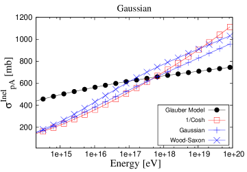
Figure 3:

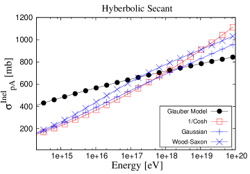
Figure 4:

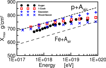
Figure 5:

References

- [1] T. Kodama et al, Does The Nuclear Heavy Ion Cross-Section Stay Constant At Ultrarelativistic Energies?, Nucl. Phys. A 523 (1991) 640-650.
- [2] M. F. Barroso,T. Kodama and Y. Hama, Reaction cross-section in ultrarelativistic nuclear collisions, Phys. Rev. C 53 (1996), 501-504.
- [3] M. Unger [The Pierre Auger Collaboration], Study of the Cosmic Ray Composition above 0.4 EeV using the Longitudinal Profiles of Showers observed at the Pierre Auger Observatory, Proc of 30th Int. Cosmic Ray Conf., Merida 4 (2007) 373-376, astro-ph/0706.1495.
- [4] A. H. Mueller, Small x Behavior and Parton Saturation: A QCD Model, Nucl. Phys. B 335 (1990) 115-137.
- [5] H. Kowalski and D. Teaney, An impact parameter dipole saturation model, Phys. Rev. D 68 (2003) 114005, hep-ph/0304189.
- [6] H. Kowalski, T. Lappi and R. Venugopalan, Nuclear enhancement of universal dynamics of high parton densities, Phys. Rev. Lett. 100 (2008) 022303, hep-ph/0705.3047.
- [7] H. Kowalski, T. Lappi, C. Marquet and R. Venugopalan, Nuclear enhancement and suppression of diffractive structure functions at high energies, Phys. Rev. C 78 (2008) 045201, hep-ph/0805.4071.
- [8] J. Bartels, K. J. Golec-Biernat and H. Kowalski, A modification of the saturation model: DGLAP evolution, Phys. Rev. D 66 (2002) 014001, hep-ph/0203258.
- [9] J. Bartels, E. Gotsman, E. Levin, M. Lublinsky and U. Maor, The dipole picture and saturation in soft processes, Phys. Lett. B 556 (2003) 114-122, hep-ph/0212284.
- [10] H. G. Dosch, E. Ferreira and A. Kramer, Nonperturbative QCD treatment of high-energy hadron hadron scattering, Phys. Rev. D 50 (1994) 1992-2015, hep-ph/9405237.
- [11] C. Avila et al. [E-811 Collaboration], The Ratio, , of the real to the imaginary part of the forward elastic scattering amplitude at = 1.8-TeV, Phys. Lett. B 537 (2002) 41-44.
- [12] F. Abe et al. [CDF Collaboration], Measurement of the total cross-section at GeV and 1800-GeV, Phys. Rev. D 50 (1994) 5550-5561.
- [13] N. A. Amos et al. [E710 Collaboration], Measurement of , the ratio of the real to imaginary part of the forward elastic scattering amplitude, at = 1.8-TeV, Phys. Rev. Lett. 68 (1992) 2433-2436.
- [14] M. Honda et al., Inelastic cross-section for p-air collisions from air shower experiment and total cross-section for p p collisions at SSC energy, Phys. Rev. Lett. 70 (1993) 525-528.
- [15] R. M. Baltrusaitis et al., Total Proton Proton Cross-Section At S**(1/2) = 30-Tev, Phys. Rev. Lett. 52 (1984) 1380-1383.
- [16] M. Gluck, E. Reya and A. Vogt, Dynamical parton distributions revisited, Eur. Phys. J. C 5 (1998) 461-470, hep-ph/9806404.
- [17] R. Ulrich, R. Engel, S. Muller, F. Schussler and M. Unger, Proton-Air Cross Section and Extensive Air Showers, hep-ph/0906.3075.
- [18] G. Bossard et al., Cosmic ray air shower characteristics in the framework of the parton-based Gribov-Regge model NEXUS, Phys. Rev. D 63 (2001) 054030, hep-ph/0009119.
- [19] H. J. Drescher and G. R. Farrar, Air shower simulations in a hybrid approach using cascade equations, Phys. Rev. D 67 (2003) 116001, astro-ph/0212018.
- [20] D. Heck, J. Knapp, J. N. Capdevielle, G. Schatz, and T. Thouw, CORSIKA: A Monte Carlo code to simulate extensive air showers, Report FZKA 6019 (1998).
- [21] T. K. Gaisser, Cosmic rays and particle physics, Cambridge, UK: Univ. Pr. (1990) 279 p, 201-202.
- [22] R. S. Fletcher, T. K. Gaisser, P. Lipari and T. Stanev, SIBYLL: An Event generator for simulation of high-energy cosmic ray cascades, Phys. Rev. D 50 (1994) 5710-5731.
- [23] L. D. McLerran and R. Venugopalan, Computing quark and gluon distribution functions for very large nuclei, Phys. Rev. D 49 (1994) 2233-2241, hep-ph/9309289.
- [24] E. Iancu, A. Leonidov and L. D. McLerran, Nonlinear gluon evolution in the color glass condensate. I, Nucl. Phys. A 692 (2001) 583-645, hep-ph/0011241.
- [25] E. Iancu and L. D. McLerran, Saturation and universality in QCD at small x, Phys. Lett. B 510 (2001) 145-154, hep-ph/0103032.
- [26] J. Jalilian-Marian, A. Kovner, L. D. McLerran and H. Weigert, The intrinsic glue distribution at very small x, Phys. Rev. D 55 (1997) 5414-5428, hep-ph/9606337.