Space and velocity distributions of Galactic isolated old Neutron stars

Abstract

I present the results of Monte-Carlo orbital simulations of Galactic Neutron Stars (NSs). The simulations take into account the up-to-date observed NS space and velocity distributions at birth, and account for their formation rate. I simulate two populations of NSs. Objects in the first population were born in the Galactic disk at a constant rate, in the past 12 Gyr. Those in the second population were formed simultaneously 12 Gyr ago in the Galactic bulge. I assume that the NSs born in the Galactic disk comprise 40% of the total NS population. Since the initial velocity distribution of NSs is not well known, I run two sets of simulations, each containing $3\times 10^{6}$ simulated NSs. One set utilizes a bimodal initial velocity distribution and the other a unimodal initial velocity distribution, both are advocated based on pulsars observations. In light of recent observational results, I discuss the effect of dynamical heating by Galactic structure on NS space and velocity distributions and show it can be neglected. I present catalogue of simulated NS space and velocity vectors in the current epoch, and catalogue of positions, distances and proper motions of simulated NSs, relative to the Sun. Assuming there are $10^{9}$ NSs in the Galaxy, I find that in the solar neighborhood the density of NSs is about $2-4\times 10^{-4}$ pc^-3, and their scale height is about $0.3-0.6$ kpc (depending on the adopted initial velocity distribution). These catalogue can be used to test the hypothesis that some radio transients are related to these objects.

1. Introduction

The present day space and velocity distributions of Galactic isolated old Neutron Stars (NS), are the subject of many studies. Among the reasons for deriving the positional and kinematical properties of isolated old NSs was the suggestion that Gamma-Ray Bursts (GRBs) may originate from Galactic NSs (e.g., Mazets et al. 1980). This was refuted by the homogeneous sky distribution of GRBs (e.g., Meegan et al. 1992), and later on by the discovery of their cosmic origin (e.g., Metzger et al. 1997; van Paradijs et al. 1997).

Another exciting possibility, that re-ignited these efforts, was to detect isolated old NSs in soft X-ray radiation that may be emitted as they slowly accrete matter from the interstellar medium (ISM; Ostriker, Rees & Silk 1970; Shvartsman 1971). Treves & Colpi (1991), and Blaes & Madau (1993) predicted that $\sim 10^{3}$–$10^{4}$ isolated old NS accreting from the ISM would be detected by the ROSAT Position Sensitive Proportional Counters (PSPC) all sky survey (Voges et al. 1999). Although intensive searches for these objects were carried out (e.g., Motch et al. 1997; Maoz, Ofek, & Shemi 1997; Haberl, Motch, & Pietsch 1998; Rutledge et al. 2003; Agüeros et al. 2006), only a handful of candidates were found. However, these are presumably young cooling NSs, rather than old NSs whose luminosity is dominated by accretion from the ISM (e.g., Neuhäuser & Trümper 1999; Popov et al. 2000; Treves et al. 2001). Apparently, the reasons for the rareness of these objects in the ROSAT source catalog is that their typical velocities were underestimated by earlier studies (i.e., Narayan & Ostriker 1990). It is also possible that their accretion rate is below the Bondi-Hoyle rate (e.g., Colpi et al. 1998; Perna et al. 2003; Toropina et al. 2001, 2003, 2005; see however Arons & Lea 1976,1980), or that these NSs are in an ejection stage (e.g., Colpi et al. 1998; Livio et al. 1998; Popov & Prokhorov 2000).

During the last several years, new classes of radio transients were found (e.g., Bower et al. 2007; Matsumura et al. 2007; Niinuma et al. 2007; Kida et al. 2008; see also Levinson et al. 2002; Gal-Yam et al. 2006). Bower et al. (2007) found several examples of these transients in a single small field of view, and showed that they have time scales above 20 min but below seven days, and they lack any quiescent X-ray, visible-light, near-Infrared (IR), and radio counterparts. Recently, Ofek et al. (2009) suggested that these transient events may be associated with Galactic isolated old NSs. However, testing this hypothesis requires knowledge of the NSs space distribution.

There are two approaches in the literature for calculating the theoretical space and velocity distributions of old NSs. Paczynski (1990), Hartmann, Woosley, & Epstein (1990), Blaes & Rajagopal (1991), Blaes & Madau (1993), and Posselt et al. (2008) carried out Monte-Carlo simulations of NS orbits. In such simulations, the positions and velocities of NS at birth are integrated assuming some non-evolving Galactic potential. A second approach is to use some sort of semi-analytic approximation in order to estimate the “final” NS space and velocity distributions. Frei, Huang, & Paczynski (1992) calculated the final vertical density and velocity distributions of NSs, assuming that the gravitational potential is a function only of the height, $z$, above the Galactic plane. Using the epicyclic approximation, Blaes & Rajagopal (1991) developed a technique that allows calculation of the full three dimensional velocity distribution of NSs. However, they showed that this method is not adequate for fast moving objects, which constitute the majority of the NS population. Blaes & Madau (1993) used the thin-disk approximation to calculate the space and velocity distributions of NSs. In this prescription, the radial motion of NSs are controlled by the Galactic potential in the Galactic disk, regardless of the vertical height, $z$, of the NS above/below the Galactic plane. Finally, another solution was presented by Prokhorov & Postnov (1994), who assume that the ergodic hypothesis is correct (see discussion in Binney & Tremaine 1987).

Madau & Blaes (1994) noted that all these approaches neglect dynamical heating of NSs due to encounters with giant molecular clouds, spiral arms, and stellar “collisions” (e.g., Kamahori & Fujimoto 1986, 1987; Barbanis & Woltjer 1967; Carlberg & Sellwood 1985; Jenkins & Binney 1990). They crudely estimated the order of magnitude of this effect by applying the force-free diffusion equation to the vertical height, $z$, and NS speed distributions. They found that, at the solar neighborhood, dynamical heating may decrease the local density of NSs by a factor of $\sim 1.5$ relative to a non-heated population.

In this paper I present the results of Monte-Carlo orbital simulations of Galactic NSs. These simulations improve upon past efforts (e.g., Paczynski 1990; Hartmann, Epstein, & Woosley 1990, Blaes & Rajagopal 1991; Blaes & Madau 1993; Popov et al. 2005; and Posselt et al. 2008) in several aspects. First, I use up-to-date space and velocity distributions of NSs at birth from Arzoumanian et al. (2002) and Faucher-Giguère & Kaspi (2006). Second, I assume a birth rate of NSs along the Galaxy life time, instead of assuming that all the NSs were born about 10 Gyr ago. Third, I generate a large sample of simulated NSs, which is about one to two orders of magnitude larger than those presented by previous efforts.

The structure of this paper is as follows: In §2 I present the model ingredients for the Monte-Carlo simulations. In §3 I discuss dynamical heating and show that it can be neglected. The Monte-Carlo simulations are described in §4, and the catalogue of simulated NSs are presented in §5. The results of these simulations are presented in §6, and in §7 I summarize the results and compare them with some of the previous efforts.

2. Model ingredients

In the following subsections, I present the ingredients of the Monte-Carlo simulations. These are: NSs birth rate (§2.1); space and velocity distributions of NSs at birth (§2.2); and the Galactic potential (§2.3).

2.1. NSs birth rate

The stellar population in the Milky Way is composed of at least two major components: a bulge and a disk. I therefore, simulate two populations of NSs. A Galactic disk-born population and a Galactic bulge population. For the Galactic-disk NSs, I assume a continuous constant formation rate in the past 12 Gyr. This assumption is motivated by the analysis of Rocha-Pinto et al. (2000) that did not find any major trends in the star formation rate in the disk of our Galaxy. I assume that the Galactic-bulge NSs were born in a single burst 12 Gyr ago (Ferreras, Wyse, & Silk 2003; Ballero et al. 2007; Minniti & Zoccali 2008).

As I discuss in this section, the simulations presented here consist of $40\%$ disk-born NSs and $60\%$ bulge-born NSs. The actual ratio of disk to bulge NSs is unknown and may be significantly different than the one assumed here. Therefore, in the resulting catalogue (§5) I specify the origin of each simulated NS and present the results also for each population separately.

The total number of NSs in the Milky Way is constrained by the chemical composition of the Galaxy. Specifically, the iron content of the Galaxy implies that the total number of core collapse supernovae (SNe; and therefore NSs) that exploded in the Milky Way is about $10^{9}$ (Arnett, Schramm, & Truran 1989). However, the star formation rate in the Galactic disk was approximately constant during the last $\sim 12$ Gyr (Rocha-Pinto et al. 2000; see also Noh & Scalo 1990). Therefore, with the current NS birth rate of up to one in 30 years (e.g., Diehl et al. 2006), one expects that there will be $\mathrel{\raise 1.29167pt\hbox{$<$}\mkern-14.0mu\lower 2.58334pt\hbox{$\sim$}}4\times 10^{8}$ disk-born NSs in our Galaxy. The predictions based on the SN rate ($\mathrel{\raise 1.29167pt\hbox{$<$}\mkern-14.0mu\lower 2.58334pt\hbox{$\sim$}}4\times 10^{8}$) and the chemical evolution ($\sim 10^{9}$) are therefore inconsistent. Ways around this problem include uncertainty in the SN rate (e.g., Arnett et al. 1989), and difficulty in estimating the star formation history of our Galaxy (Keane & Kramer 2008). Another viable resolution of this discrepancy is that the Galactic bulge had a higher star formation rate at earlier times.

The Galactic bulge contains a considerable number of stars that were born, apparently, in a $\sim 1$ Gyr-long, burst about 12 Gyr ago (Ferreras, Wyse, & Silk 2003; Ballero et al. 2007; Minniti & Zoccali 2008). I therefore, assume here that in addition to the disk-born NSs there are up to $6\times 10^{8}$ NSs that were formed in the Galactic bulge about 12 Gyr ago. This number was selected such that the total number of NSs in the Galaxy is $10^{9}$.

I note that the Galactic bulge contains only about 20% of the Galactic stars (e.g., Klypin et al. 2002). However, Ballero et al. (2007) argued that the initial mass function, $dN/dM$, of the bulge is skewed toward high masses, with $x$, the power-law index in the stellar mass function ($dN/dM\propto M^{-(1+x)}$; e.g., Salpeter 1955), being $<0.95$. Assuming that stars with masses exceeding 8 M_⊙ produce NSs within a relatively short time after their birth, this suggests that the number of NSs born in the Galactic bulge is a few times larger than the number of NSs born in the Galactic disk, per unit stellar mass. Therefore, the assumption that the majority of NSs were born in the Galactic bulge is in rough agreement with the expected fraction of high mass ($\mathrel{\raise 1.29167pt\hbox{$>$}\mkern-14.0mu\lower 2.58334pt\hbox{$\sim$}}8$ M_⊙) stars in the bulge, relative to the disk. Nevertheless, as stated before, the ratio between the numbers of bulge-born to disk-born NSs is uncertain. The simulations presented here cover a wide range of possibilities regarding birth place and time scenarios.

2.2. NSs space and velocity distributions at birth

Following, Paczynski (1990), I adopt a radial birth probability distribution, $p(R)$, which follows the exponential stellar disk:

$$dp(R)=a_{R}\frac{R}{R_{d}^{2}}\exp{\Big{(}-\frac{R}{R_{d}}\Big{)}}dR,$$ (1)

where $R$ is the distance from the Galactic center projected on the Galactic plane, $R_{d}=4.5$ kpc is the exponential disk scale length, and $a_{R}$ is the normalization given by:

$$a_{R}=[1-e^{-R_{max}/R_{d}}(1+R_{max}/R_{d})]^{-1},$$ (2)

where $R_{max}=15$ kpc, is the disk truncation radius. Yusifov & Küçük (2004) estimated the radial distribution (measured from the Galactic center) of Galactic pulsars, and found it to be more concentrated than predicted by the Paczynski (1990) distribution. However, I note that the supernova remnant Galactic radial distribution is in good agreement with the Paczynski (1990) model.

For the NS bulge population I assume that the space distribution at birth has the same functional form and parameters as the NS disk population, but with $R_{d}=1$ kpc in Eqs. 1 and 2.

For the initial velocity probability distribution, I use two different models. Both models are consistent with the observed velocity distribution of young pulsars. One is a bimodal velocity distribution composed of two Gaussians found by Arzoumanian et al. (2002), and the second is based on a double-sided exponential unimodal velocity distribution (Faucher-Giguère & Kaspi 2006).

Bimodal velocity distribution: The first initial velocity distribution we used is from Arzoumanian et al. (2002). It consists of two components. The three-dimensional speed, $v$, probability density of this model is:

$$p(v)=4\pi v^{2}\sum_{j=1,2}{\frac{f_{j}}{(2\pi\sigma_{v,j}^{2})^{3/2}}\exp{(-v^{2}/[2\sigma_{v,j}^{2}])}}$$ (3)

where $j\in\{1,2\}$, $f_{1}=0.40$ and $f_{2}=0.60$ are the fractions of the two NS velocity components, $\sigma_{v,1}=90$ km s^-1, and $\sigma_{v,2}=500$ km s^-1.

Unimodal velocity distribution: The second model I use for the velocity distribution of NSs at birth was advocated by Faucher-Giguère & Kaspi (2006). In their model, each one-dimensional (projected) velocity component, $v_{i}$, consists of a double-sided exponential probability distribution:

$$p(v_{i})=\frac{1}{2\langle v_{i}\rangle}\exp{\Big{(}-\frac{|v_{i}|}{\langle v_{i}\rangle}\Big{)}},$$ (4)

where $\langle v_{i}\rangle=180$ km s^-1 is the mean velocity in each direction, $i$. I note that drawing the velocity components of simulated NSs directly from Eq. 4 will result in an aspherical distribution. In order to avoid this problem the corresponding three-dimensional distribution is required. Faucher-Giguère & Kaspi (2006) noted that this distribution is difficult to derive analytically, and did not provide its functional form. However, it is possible to show that the corresponding spherically symmetric three-dimensional distribution corresponding to Eq. 4 is given by

$$p(v)=\frac{v}{\langle v_{i}\rangle^{2}}\exp{\Big{(}-\frac{|v|}{\langle v_{i}\rangle}\Big{)}}.$$ (5)

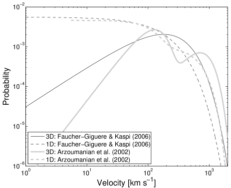
In Figure 1 I show the one-dimensional (dashed lines) and three-dimensional (solid lines) initial velocity probability distributions based on Faucher-Giguère & Kaspi (2006) velocity distribution (thin black lines) and the Arzoumanian et al. (2002) distribution (thick gray lines). Several other fits for the pulsars velocity distribution at birth are available (e.g., Hansen & Phinney 1997; Cordes & Chernoff (1998); Hobbs et al. 2005; Zou et al. 2005). However, the Arzoumanian et al. (2002) and Faucher-Giguère & Kaspi (2006) velocity distributions cover a wide range of possibilities, that reflect the current uncertainties in the pulsars velocity distribution at birth.

The two models are considerably different from each other, mainly in the low and high velocity tails. Relative to the Arzoumanian et al. (2002) velocity distribution the Faucher-Giguère & Kaspi (2006) distribution has excess of NSs at low velocities. Since the slowest NSs are the most efficient accretors from the ISM (e.g., Ostriker et al. 1970), these differences may have a significant impact on the detectability of isolated old NSs in X-ray wavebands (e.g., Blaes & Madau 1993).

Figure 1.— The initial velocity distribution of NSs at birth relative to a rotating galaxy. The dashed lines represent the one-dimensional (1D) velocity distributions, while the solid lines show the three-dimensional (3D) speed distributions. The black thin lines are for the Faucher-Giguère & Kaspi (2006) unimodal double-sided exponential velocity distribution, while the gray thick lines show the Arzoumanian et al. (2002) bimodal Gaussian velocity distribution.

The velocity distributions, in Eqs. 3 and 5, are given relative to a rotating disk. Therefore, I added the disk rotation velocity to these birth velocities

$$v^{\prime}_{x}=v_{x}-V_{circ}(R)\sin(\theta),$$ (6)

$$v^{\prime}_{y}=v_{y}+V_{circ}(R)\cos(\theta),$$ (7)

$$v^{\prime}_{z}=v_{z},$$ (8)

where $v_{i}$ is the velocity vector relative to the rotating disk (i.e., the one obtained from Eqs. 3 or 5), $v^{\prime}_{i}$ is the velocity vector in a non-rotating (inertial) reference frame, $R=(x^{2}+y^{2})^{1/2}$, $\theta$ is azimuthal angle on the Galactic disk ($={\rm arctan2}[y,z]$), which was selected from a uniform random distribution, and $x$, $y$, and $z$ are the position in a Cartesian, non-rotating, coordinate system, whose origin is the Galactic center, and $z$ is vertical to the Galactic plane. Finally, $V_{circ}$ was obtained from

$$V_{circ}(R)=\sqrt{-R\nabla_{R}{\Phi}},$$ (9)

where $\Phi$ is the Galactic potential (see §2.3), at the point of interest.

Finally, I assume that the vertical height above the Galactic mid-plane of NSs at birth, $z$, is drawn from a Gaussian distribution ($\propto\exp[-z^{2}/(2\sigma_{b})]$), with $\sigma_{b}=0.16$ kpc and $0.05$ kpc, for the Arzoumanian et al. (2002) and Faucher-Giguère & Kaspi (2006) initial velocity distributions, respectively.

2.3. The Galactic potential

Following Paczynski (1990), I assume that the Galactic potential is composed of a disk component, an spheroidal component, and an halo component. I also added a central black hole component.

The disk and spheroid components are described by the following potential proposed by Miyamoto & Nagai (1975),

$$\Phi_{k}(x,y,z)=-\frac{GM_{k}}{\Big{\{}x^{2}+y^{2}+[a_{k}+(z^{2}+b_{k}^{2})^{1/2}]^{2}\Big{\}}^{1/2}},$$ (10)

where $a_{k}$, $b_{k}$ and $M_{k}$ are given in Equations 13 and 14, and where $k=d$ corresponds to the disk component and $k=s$ corresponds to the spheroid component, and $G$ is the Gravitational constant. Next, the halo potential is given by

$$\Phi_{h}(r)=-\frac{GM_{h}}{r_{h}}\Big{[}\frac{1}{2}\ln{\Big{(}1+\frac{r^{2}}{r_{h}^{2}}\Big{)}}+\frac{r_{h}}{r}\arctan{\Big{(}\frac{r}{r_{h}}\Big{)}}\Big{]},$$ (11)

were $r^{2}=x^{2}+y^{2}+z^{2}$, $M_{h}$, and $r_{h}$ are listed in Eq. 15. Furthermore, I added a component representing the Galactic central massive black-hole (e.g., Ghez et al. 1998):

$$\Phi_{bh}(r)=-\frac{GM_{bh}}{r},$$ (12)

where $M_{bh}$ is given in Eq. 16 (Eisenhauer et al. 2005). The choice of parameters listed here reproduces the observed Galactic rotation, local density, and local column density (see Paczynski 1990 for details):

$$a_{d}=3.7~{}{\rm kpc},~{} b_{d}=0.20~{}{\rm kpc},~{} M_{d}=8.07\times 10^{10}~{}{\rm M_{\odot}},$$ (13)

$$a_{s}=0.0~{}{\rm kpc},~{} b_{s}=0.277~{}{\rm kpc},~{} M_{s}=1.12\times 10^{10}~{}{\rm M_{\odot}},$$ (14)

$$r_{h}=6.0~{}{\rm kpc},~{} M_{h}=5.0\times 10^{10}~{}{\rm M_{\odot}},$$ (15)

$$M_{bh}=3.6\times 10^{6}~{}{\rm M_{\odot}}.$$ (16)

I note that the black hole contributes about $4\%$ ($0.6\%$) of the gravitational potential at distance of 1 pc (10 pc) from the black hole. Therefore, its influence on the Galactic potential is negligible and it does not change the fitted parameters in Eqs. 13-16. However, it may heat NSs passing nearby. Finally, the Galactic potential is the sum of these four components:

$$\Phi=\Phi_{d}+\Phi_{s}+\Phi_{h}+\Phi_{bh}.$$ (17)

3. Dynamical Heating

Dynamical heating, presumably by giant molecular clouds (e.g., Kamahori & Fujimoto 1986; 1987), spiral structure (e.g., Barbanis & Woltjer 1967; Carlberg & Sellwood 1985; Jenkins & Binney 1990), and stars, tends to broaden the velocity and spatial distributions of Galactic stars (e.g., Wielen 1977; Nordstrom et al. 2004).

In order to roughly estimate the effect of dynamical heating on NSs, Madau & Blaes (1994) applied the force-free diffusion equation to the velocity and vertical distance distributions of NSs. They adopted the total diffusion coefficient, $C$ ($=C_{U}+C_{V}+C_{W}$), measured by Wielen (1977; $C=600$ km² s^-2 Gyr^-1). In this, $U$ corresponds to the radial direction, and is positive in the direction of the Galactic center; $V$ points in the direction of circular rotation; and $W$ is directed towards the North Galactic pole. Applying heating, they found that the local density of NSs is smaller by about 30% relative to the case of no heating. In the following we discuss this approach in light of new observational data available.

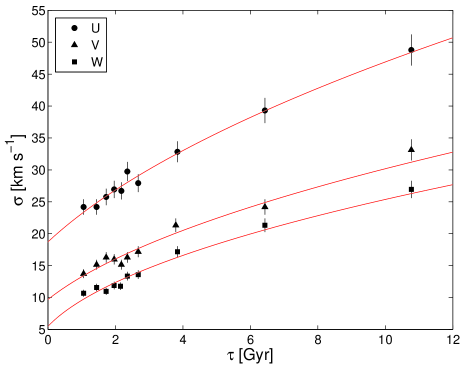
We estimate the diffusion coefficient, $C$, using modern data. Nordstrom et al. (2004), estimated the dynamical heating by the Galactic disk and showed that it does not saturate after some time as suggested by measurements based on smaller samples (e.g., Quillen & Garnett 2001; see also Aumer & Binney 2009). Approximating dynamical heating by a random walk process, I fit the Nordstrom et al. (2004) measurements with the function (e.g., Wielen 1977)

$$\sigma_{g}=(\sigma_{g,0}^{2}+C_{g}\tau)^{1/2},$$ (18)

where $\sigma_{g}$ is the velocity dispersion component at time, $\tau$, since birth, $\sigma_{g,0}$ is the initial velocity dispersion component and $g\in(U,V,W)$. The data and the best fit curves are shown in Figure 2, and the best fit parameters are listed in Table 1.

Figure 2.— Stellar velocity dispersion ($\sigma$) along the $U$ (radial; circles), $V$ (tangential; triangles) and $W$ (vertical; squares) Galactic directions as a function of age since birth, $\tau$, as measured by Nordstrom et al. (2004). The lines represent the best fit of Equation 18 to the data. The best fit parameters are listed in Table 1.

Table 1The Galactic disk diffusion coefficients

Velocity component	$\sigma_{g,0}$	$C$	$\chi^{2}/dof$
	km s-1	km2 s-2 Gyr-1
U	$18.7\pm 1.2$	$185\pm 19$	$3.1/8$
V	$9.7\pm 0.9$	$81.7\pm 7.5$	$9.3/8$
W	$5.5\pm 1.0$	$61.3\pm 5.1$	$11.0/8$

Note. — The diffusion coefficients of Galactic stars as obtained by fitting Eq. 18 with the measurements of Nordstrom et al. (2004).

The total diffusion coefficient that I find, $C_{U}+C_{V}+C_{W}=328\pm 21$ km² s^-2 Gyr^-1, is about half of the value found by Wielen (1977), and used by Madau & Blaes (1994).

Next, the initial velocities estimated by Narayan & Ostriker (1990), that was used by Madau & Blaes (1994), are considerably lower than the more recent estimates (e.g., Arzoumanian et al. 2002). As suggested by Eq. 18, diffusion affects mostly low velocity objects. Therefore, dynamical heating is less important than estimated by Madau & Blaes (1994).

Furthermore, the approach taken by Madau & Blaes (1994) assumes that NSs are being affected by diffusion at all times. However, the scatterers are restricted to the Galactic plane. NSs are born with high velocities and spend $80\%$ to $90\%$ of the time at distances larger than 100 pc from the Galactic plane (based on the results in §6). Therefore, they are less susceptible to dynamical heating than disk stars. Based on these three arguments, I conclude that the importance of dynamical heating was over estimated by Madau & Blaes (1994) by at least an order of a magnitude.

Nevertheless, dynamical heating may effect some of the slow moving objects, but they are a minority among the Galactic NSs. Eq. 18 roughly suggests that dynamical heating is important for NSs with speeds smaller than about $(C\tau)^{1/2}$. Even for $\tau=10$ Gyr this gives 60 km s^-1. However, only $2.8\%$ and $4.5\%$ of the NSs in the Arzoumanian et al. (2002) and Faucher-Giguère & Kaspi (2006), initial velocity distributions, respectively, have speeds smaller than 60 km s^-1 at birth (relative to their local standard of rest).

4. Monte-Carlo simulations

To solve for NS orbits I integrate the equations of motion

$$\frac{d^{2}\vec{x}}{dt^{2}}=-\vec{\nabla}\Phi,$$ (19)

using a Livermore ordinary differential equation solver (Hindmarsh 1983). The integration is performed in a non-rotating, Cartesian coordinates system, the origin of which is the Galactic center, and the $z$ axis is perpendicular to the Galactic plane.

For each initial velocity distribution (i.e., bimodal or unimodal; see §2.2), I simulated $3\times 10^{6}$ NS orbits. In each simulation I randomly drew the NSs birth times, positions, and velocities, from the probability distributions described in §2.1, and §2.2. As explained before, $40\%$ of these NSs are disk-born, and the rest are bulge-born.

At the end of each simulation I checked if the integration conserved the total energy. In cases in which the energy was not conserved to within $0.1\%$, I reran the integration using the same initial conditions, with a refined integration tolerance. In the second (and final) iteration, the energy was conserved to better than $2.8\%$ in all cases.

5. Catalogue

The catalogue of initial (i.e., at birth) and final (i.e., current epoch) simulated NSs space and velocity components are listed in Table 2 for the bimodal initial velocity distribution of Arzoumanian et al. (2002), and in Table 3 for the unimodal initial velocity of Faucher-Giguère & Kaspi (2006). The first column in each table indicates whether the simulated NS belongs to the bulge population (code 0) or disk population (code 1).

Table 2NS Monte-Carlo orbital simulations using the bimodal initial velocity distribution

Initial									Final
P	Age	$X$	$Y$	$Z$	$\dot{X}$	$\dot{Y}$	$\dot{Z}$	$V_{circ}$	$X$	$Y$	$Z$	$\dot{X}$	$\dot{Y}$	$\dot{Z}$
	Gyr	kpc	kpc	kpc	kpc Gyr-1	kpc Gyr-1	kpc Gyr-1	kpc Gyr-1	kpc	kpc	kpc	kpc Gyr-1	kpc Gyr-1	kpc Gyr-1
0	12.0	$-2.04$	$1.16$	$-0.07$	$-77.7$	$-194.6$	$8.8$	$208.7$	$-0.71$	$2.41$	$-0.07$	$-181.0$	$-70.7$	$9.1$
0	12.0	$-0.58$	$1.57$	$-0.27$	$-199.1$	$0.1$	$-376.7$	$206.7$	$-1.40$	$-8.23$	$-5.08$	$42.4$	$25.4$	$-70.3$
0	12.0	$0.60$	$1.57$	$0.02$	$531.9$	$507.1$	$-60.9$	$206.6$	$477.31$	$404.37$	$-5.35$	$-154.9$	$-132.3$	$2.3$
0	12.0	$-1.27$	$2.33$	$0.05$	$-140.6$	$-96.1$	$-53.5$	$211.6$	$-0.20$	$2.64$	$0.06$	$-167.7$	$-32.5$	$52.4$
0	12.0	$-1.54$	$-2.95$	$-0.18$	$-137.7$	$-209.2$	$-425.3$	$218.2$	$-1.31$	$-1.29$	$-19.70$	$-10.4$	$53.7$	$251.2$

Note. — Catalog of initial and final space positions and velocity components for $3\times 10^{6}$ simulated NSs. The NSs were simulated using the bimodal initial velocity distribution of Arzoumanian et al. (2002). The velocity components are given in kpc Gyr^-1, relative to the non-rotating Galaxy. In order to convert kpc Gyr^-1 to km s^-1, divide it by $1.0227$. P is the population type: 0 for bulge-born NS; 1 for disk-born NS. $V_{circ}$ refers to the Galaxy rotation speed at the projected location, on the Galactic disk, in which the NS was born. The initial (and final) velocity components are given relative to a non-rotating galaxy (inertial reference frame). The numbers in this table are rounded in order to fit into the page. This table is published in its entirety in the electronic edition of this paper. A portion of the full table is shown here for guidance regarding its form and content.

Table 3NS Monte-Carlo orbital simulations using the unimodal initial velocity distribution

Initial									Final
P	Age	$X$	$Y$	$Z$	$\dot{X}$	$\dot{Y}$	$\dot{Z}$	$V_{circ}$	$X$	$Y$	$Z$	$\dot{X}$	$\dot{Y}$	$\dot{Z}$
	Gyr	kpc	kpc	kpc	kpc Gyr-1	kpc Gyr-1	kpc Gyr-1	kpc Gyr-1	kpc	kpc	kpc	kpc Gyr-1	kpc Gyr-1	kpc Gyr-1
1	2.3	$-7.05$	$-6.69$	$0.07$	$-258.0$	$-232.1$	$-55.2$	$220.2$	$-39.41$	$-3.21$	$-5.51$	$24.9$	$4.3$	$8.8$
0	12.0	$0.38$	$0.88$	$-0.01$	$-124.3$	$-176.5$	$134.8$	$226.7$	$0.35$	$0.10$	$0.60$	$213.6$	$178.4$	$79.1$
1	2.9	$-0.69$	$5.40$	$0.07$	$-124.5$	$122.9$	$294.4$	$227.1$	$-6.97$	$-5.47$	$-11.00$	$34.2$	$-57.3$	$105.9$
1	0.6	$-2.02$	$-1.49$	$-0.02$	$-510.5$	$-374.6$	$5.6$	$210.2$	$-140.81$	$-103.14$	$-0.48$	$-139.0$	$-101.7$	$-0.8$
0	12.0	$-2.34$	$-2.96$	$-0.02$	$178.0$	$-374.0$	$-108.7$	$221.6$	$-7.62$	$-17.92$	$2.54$	$115.5$	$87.9$	$-21.8$

Note. — Like Table 2, but for the unimodal initial velocity distribution of Faucher-Giguère & Kaspi (2006).

In addition, catalogue of simulated NS positions, distances, radial velocities, and proper motions for an observer located at the “solar circle”, moving around the Galactic center with a velocity of 220 km s^-1 is given in tables 4 and 5. The solar circle is defined to be on the Galactic plane (i.e., $z=0$ kpc) at the distance of the Sun from the Galactic center ($R_{\odot}=8.0$ kpc; Ghez et al. 2008). The catalogue in Tables 4 and 5 are based on the initial velocity distribution of Arzoumanian et al. (2002) and the Faucher-Giguère & Kaspi (2006), respectively. I note that the radial velocity and proper motions are calculated for a static observer with respect to the Local Standard of Rest (LSR; i.e., the solar motion with respect to the LSR is neglected).

In order to reduce Poisson errors in the local properties of NSs (i.e., density; sky surface density), tables 4 and 5 were produced by calculating the positions of the $3\times 10^{6}$ simulated NSs in tables 2 and 3, respectively, from 100 random locations on the solar circle. Hence, tables 4 and 5 list $3\times 10^{8}$ simulated NSs.

Table 4Catalog of simulated NSs as observed from the LSR - based on the bimodal initial velocity distribution

P	Age	$l$	$b$	dist	$\mu_{l}$	$\mu_{b}$	RV
	Gyr	deg	deg	kpc	′′ yr-1	′′ yr-1	km s-1
0	12.0000	$354.72497$	$-0.39865$	$10.0003$	$-0.0064166$	$0.0001654$	$-149.7$
0	12.0000	$72.14501$	$-38.10227$	$8.2258$	$-0.0025465$	$-0.0041258$	$-93.8$
0	12.0000	$273.07904$	$-0.49003$	$625.9548$	$-0.0000573$	$0.0000017$	$340.7$
0	12.0000	$351.53160$	$0.34229$	$9.9375$	$-0.0057996$	$0.0011040$	$-124.8$
0	12.0000	$13.81616$	$-68.84354$	$21.1283$	$-0.0015999$	$0.0004210$	$-247.1$

Note. — Catalog of Galactic longitudes ($l$), latitudes ($b$), distances, proper motions in Galactic longitude ($\mu_{l}$) and latitude ($\mu_{b}$), and radial velocities (RV) from a point on the solar circle (e.g., the LSR) of $3\times 10^{8}$ simulated NSs. The velocities and proper motions do not include the motion of the Sun relative to the LSR. The proper motions are given in the Galactic coordinate system. The catalog was generated by calculating the positions of the $3\times 10^{6}$ NSs in Table 2 (i.e., assuming the Arzoumanian et al. [2002] initial velocity distribution) as observed from 100 random points on the solar circle. The conversion of space velocity to proper motion and radial velocity was carried out using the inverse of Eq. 3.23-3 in Seidelmann (1992, p. 121). This table is published in its entirety in the electronic edition of this paper. A portion of the full table is shown here for guidance regarding its form and content.

Table 5Catalog of simulated NSs as observed from the LSR - based on the unimodal initial velocity distribution

P	Age	$l$	$b$	dist	$\mu_{l}$	$\mu_{b}$	RV
	Gyr	deg	deg	kpc	′′ yr-1	′′ yr-1	km s-1
1	2.2753	$237.98450$	$-8.95638$	$35.3986$	$0.0008045$	$0.0002084$	$166.7$
0	12.0000	$2.28569$	$4.42334$	$7.8361$	$-0.0014499$	$0.0016472$	$212.2$
1	2.8584	$306.10398$	$-45.37962$	$15.4574$	$-0.0018509$	$0.0033513$	$96.8$
1	0.6194	$262.62769$	$-0.15823$	$173.4066$	$-0.0001141$	$0.0000002$	$334.3$
0	12.0000	$308.68736$	$6.21614$	$23.4368$	$0.0000392$	$-0.0003617$	$171.9$

Note. — Like Table 5, but for the unimodal initial velocity distribution of Faucher-Giguère & Kaspi (2006).

6. Statistical properties

In this section I present the space and velocity distributions of simulated NSs, at the current epoch. In §6.1 I discuss the overall distribution of NSs in the Galaxy, while in §6.2 I discuss their statistical properties as observed from the LSR. Additional specific statistical properties of these objects are discussed in Ofek et al. (2009) in the context of the long-duration radio transients (Bower et al. 2007; Kida et al. 2008). The results presented in this section assume there are $N_{9}=N/10^{9}$ NSs in the Galaxy, where $N$ is the number of NSs in the Galaxy, of which $40\%$ were born in the disk and $60\%$ in the bulge.

6.1. Overall properties

NSs are born with large space velocities, which are typically of the order of the escape velocity from the Galaxy. These are presumably the result of kick velocities due to asymmetric supernovae explosions (e.g., Blaauw 1961 ; Lai et al. 2006). Therefore, it is expected that a large fraction of the Galactic NSs will be unbounded to the Milky Way gravitational potential and some may be found at very large distances.

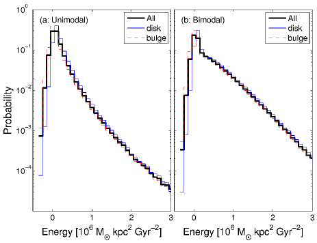
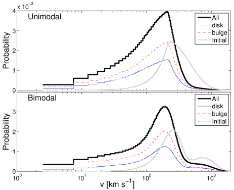
In Figure 3, I show the distribution of the total (kinetic $+$ potential) energy of the simulated NSs: $M_{NS}(v^{2}/2+\Phi)$, where the NSs mass was set to $M_{NS}=1.4$ M_⊙. Panel (a) shows the energy distribution based on the simulations using the unimodal initial velocity distribution of Faucher-Giguère & Kaspi (2006), while panel (b) is for the bimodal distribution of Arzoumanian et al. (2002). In each panel, the thick black solid line represents the entire NS population, the thin solid line shows the disk-born NSs, and the dashed line is for bulge-born NSs.

Figure 3.— The total energy distribution of Galactic-born NSs. The energy does not include external potentials (i.e., other galaxies), and assumes all NSs have a mass of 1.4 M_⊙. The different lines shows the distribution of all the NSs (solid thick black lines); only disk-born NSs (solid thin lines); and only bulge-born NSs (dashed lines).

Using the approximation that all the NSs with negative energies are gravitationally bounded to the Galaxy (neglecting heating), in Table 6 I give the fractions of NSs bounded to the Galactic gravitational potential.

Table 6Fraction of NSs gravitationally bounded to the Galaxy

Initial velocity	All	disk	bulge
A2002	0.38	0.16	0.52
FK2006	0.30	0.13	0.41

Given the large fraction of gravitationally-unbounded NSs, it is expected that some NSs may be found at very large distances, $r$, from the Galactic center. I find that about $12\%$ and $35\%$ of the NSs born in the Galaxy are currently at distances larger than 1 Mpc from the Galactic center, for the unimodal and bimodal initial velocity distributions, respectively. For $1$ Mpc$<r<10$ Mpc, I find that the density of NSs as a function of $r$ is about: $1.9\times 10^{-5}(r/1{\rm kpc})^{-2.4}N_{9}$ pc^-3 and $3.6\times 10^{-6}(r/1{\rm kpc})^{-2.1}N_{9}$ pc^-3, for the bimodal and unimodal initial velocity distributions, respectively. Finally, I find that some Milky Way born NSs may be at distances as large as 30 to 40 Mpc from the Galaxy. I note that the local density, in our Galaxy, of NSs born in other galaxies, is of the order of $10^{-11}N_{9}$ pc^-3. This was estimated by calculating the density in the the Milky Way, of NSs born in each galaxy found within 10 Mpc. For this, I used a version of the Tully (1988) nearby galaxy catalog (Ofek 2007) where the total number of NSs in each galaxy was normalized by its total $B$-band magnitude, relative to Milky Way.

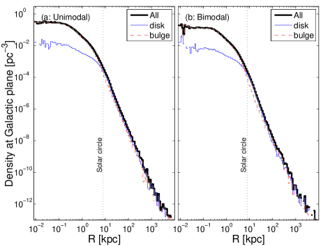
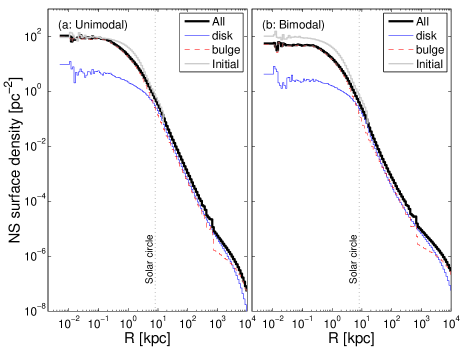
In Figures 4 and 5 I show the density of NSs on the Galactic plane, and the surface density of NSs projected on the Galactic plane, respectively, as a function of distance from the Galactic center. The notations are the same as in Figure 3. In addition, in Fig. 5, the gray solid line represents the initial surface distribution of all NSs. Furthermore, the vertical dashed lines mark the distance of the Sun from the Galactic center, $R_{\odot}=8.0$ kpc (Ghez et al. 2008). As noted before, I refer to this distance from the Galactic center, when located on the Galactic plane, as the solar circle. The densities in the solar circle and Galactic center are listed in the figure captions. I note that the fluctuations seen in small and large radii are due to Poisson noise.

Figure 4.— Density of NSs at the Galactic plane, as measured at the current epoch. See Fig. 3 for details regarding line types. The density is calculated by counting the NSs within 100 pc from the Galactic plane, dividing it by the appropriate volume in each bin, and assuming that the total number of NSs in the Galaxy is $10^{9}$. For the initial velocity distribution of Faucher-Giguère & Kaspi (2006; panel a), the NSs density at the solar circle (distance of 8.0 kpc from the Galactic center; Ghez et al. 2008) is $4.0\times 10^{-4}N_{9}$ pc^-3, of which $60\%$ are disk born and $40\%$ are bulge born. The NSs density at the Galactic center is: $3\times 10^{-1}N_{9}$ pc^-3, of which $5\%$ are disk born and $95\%$ are bulge born. For the initial velocity distribution of Arzoumanian et al. (2002; panel b), the density at the solar circle is $2.4\times 10^{-4}N_{9}$ pc^-3, of which $66\%$ are disk born and $34\%$ are bulge born. The density at the Galactic center is: $2\times 10^{-1}N_{9}$ pc^-3, of which $7\%$ are disk born and $93\%$ are bulge born. I note that the fluctuations seen in small and large radii are due to Poisson noise.

Figure 5.— The surface density of NSs projected on the Galactic plane, as measured at the current epoch. See Fig. 3 for details. In addition the gray lines show the initial surface density distributions. For the initial velocity distribution of Faucher-Giguère & Kaspi (2006; panel a), the NSs surface density at the solar circle is $0.6N_{9}$ pc^-2 of which $54\%$ are disk born NSs, and $46\%$ are bulge-born NSs. The surface density at the Galactic center is $\sim 90N_{9}$ pc^-2 of which about $9\%$ are disk born NSs, and the rest are bulge-born NSs. For the initial velocity distribution of Arzoumanian et al. (2002; panel b), the NSs density at the solar circle is $0.4N_{9}$ pc^-2 of which $61\%$ are disk born NSs, and $39\%$ are bulge-born NSs. The corresponding surface density at the Galactic center is $\sim 50N_{9}$ pc^-2 of which $\sim 6\%$ are disk born NSs, and the rest are bulge-born NSs. As before, the plotted densities assume the total number of NSs is $10^{9}$.

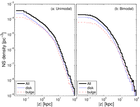
In Figure 6 I show the NSs density as a function of height above or below the Galactic plane, as measured at the solar circle. This was calculated by counting the number of simulated NSs with distance from the Galactic center, projected on the Galactic plane, of $8.0\pm 0.5$ kpc. The line scheme is the same as in Figures 3. At the solar circle the scale height of NSs is about $0.6$ kpc and $0.3$ kpc for the Arzoumanian et al. (2002) and Faucher-Giguère & Kaspi (2006) initial velocity distributions, respectively.

Figure 6.— The density of NSs as a function of height, $z$, above/below the Galactic plane as measured on the solar circle at the current epoch. Line types are like those in Fig. 3. For the initial velocity distribution of Faucher-Giguère & Kaspi (2006; panel a), $50\%$ ($90\%$) of the NSs are found within 0.9 kpc (5.6 kpc) from the Galactic plane. For the initial velocity distribution of Arzoumanian et al. (2002; panel b), $50\%$ ($90\%$) of the NSs are found within 0.7 kpc (4.4 kpc) from the Galactic plane.

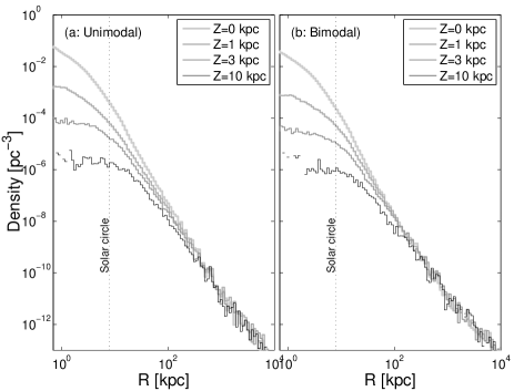
Shown in Fig. 7 are the space densities of NSs as a function of projected (on the Galactic plane) distance from the Galactic center, for several different Galactic height: 0 kpc; 1 kpc; 3 kpc; and 10 kpc. The densities are calculated in slices, parallel to the Galactic plane, with semi-width of 0.1 kpc.

Figure 7.— The density of NSs in Galactic heights of 0 kpc, 1 kpc, 3 kpc, and 10 kpc above/below the Galactic plane, as a function of the projected (on the Galactic plane) distance from the Galactic center, $R$, and as measured at the current epoch. Panel (a) shows the densities calculated using the initial velocity distribution of Faucher-Giguère & Kaspi (2006). For this model, at the solar circle, the densities are about $4\times 10^{-4}N_{9}$ pc^-3, $6\times 10^{-5}N_{9}$ pc^-3, $2\times 10^{-5}N_{9}$ pc^-3, and $2\times 10^{-6}N_{9}$ pc^-3, at Galactic heights of 0 kpc, 1 kpc, 3 kpc, and 10 kpc, respectively. Panel (b) shows the densities calculated using the initial velocity distribution of Arzoumanian et al. (2002). For this model, at the solar circle, the densities are about $2\times 10^{-4}N_{9}$ pc^-3, $5\times 10^{-5}N_{9}$ pc^-3, $1\times 10^{-5}N_{9}$ pc^-3, and $1\times 10^{-6}N_{9}$ pc^-3, at Galactic heights of 0 kpc, 1 kpc, 3 kpc, and 10 kpc, respectively.

Finally, in Figure 8 I show the initial and final speed distributions as measured relative to an inertial reference frame (contrary to Fig. 1 which shows the initial speed distribution relative to a rotating reference frame). The probabilities in this Figure are shown per 1 km s^-1 bins. The line scheme is again like the one used in Fig. 5. As expected, the typical speeds of NSs decrease with time as they, on average, increase their distances from the Galaxy and lose kinetic energy. For the unimodal initial velocity distribution, at the current epoch I estimate that about $17\%$, $53\%$, and $99\%$ of the NSs have speeds below 100, 200, and 1000 km s^-1, respectively. For the bimodal initial velocity distribution, at the current epoch I estimate that about $11\%$, $39\%$, and $94\%$ of the NSs have speeds below 100, 200, and 1000 km s^-1, respectively.

Figure 8.— The initial and final speed probability distributions of the simulated NSs, relative to an inertial reference frame. Line types are like those in Fig. 5. The probabilities are calculated for 1 km s^-1 bins. Panel (a) shows the results for the unimodal initial velocity distribution, while panel (b) for the bimodal initial velocity distribution.

6.2. Properties observed from the LSR

In this subsection I discuss: (i) the expectancy distance of the nearest NS to the Sun; (ii) the number of young NSs in the solar neighborhood; (iii) the proper motion distribution of nearby NSs; and (iv) the all-sky distribution of Galactic NSs.

The probability to find a NS within distance $d$ from the Sun is given by

$$P_{<d}=1-\exp(-\frac{4}{3}\pi\rho d^{3}).$$ (20)

Given the local density of NSs, $\rho$, that I have found in §6.1, this implies that the expectancy distance of the nearest NS is about $8.8N_{9}^{-1/3}$ pc and $7.5N_{9}^{-1/3}$ pc for the Arzoumanian et al. (2002) and Faucher-Giguère & Kaspi (2006) distributions, respectively.

For the bimodal initial velocity distribution (Table 4), within 1 kpc from the Sun, 63% of the NSs are disk-born, and there are about $220N_{9}$ ($900N_{9}$) NSs younger than 1 Myr (10 Myr). On the other hand, for the unimodal initial velocity distribution (Table 5), within 1 kpc from the Sun, 57% of the NSs are disk-born, and there are about $190N_{9}$ ($930N_{9}$) NSs younger than 1 Myr (10 Myr).

In Figure 9, I show the median total proper motion (solid lines) of simulated NSs as a function of their distance from an observer located on the solar circle. The dotted lines show the lower and upper $95$-percentiles of the proper motion distributions. The black lines represent the unimodal initial velocity distribution and the gray lines are for the bimodal initial velocity distribution. In addition, the dots show the observed proper motions of known pulsars (Manchester et al. 2005).

Figure 9.— The median total proper motion (solid lines) of simulated NSs as a function of their distance from an observer located on the solar circle. The dotted lines show the lower and upper $95$-percentiles of the proper motion distributions. The black lines represent the unimodal initial velocity distribution and the gray lines are for the bimodal initial velocity distribution. In addition, the dots show the observed proper motion of known pulsars.

Figure 10.— Sky surface density distribution of NSs, at the current epoch, for an observer located on the solar circle. The maps are presented using the Aitoff equal area projection. The grids represent Galactic coordinates with $15^{\circ}$ spacing. The panels in the left column are for the unimodal initial velocity distribution of Faucher-Giguère & Kaspi (2006), while the right column is for the bimodal initial velocity distribution of Arzoumanian et al. (2002). The upper row is assuming $10^{9}$ NSs of which $60\%$ are bulge born and $40\%$ are disk born. The middle row is for the disk born NSs, assuming there are $4\times 10^{8}$ of them in the Galaxy, while the bottom row is for the bulge born NSs, assuming there are $6\times 10^{8}$ of them in the Galaxy.

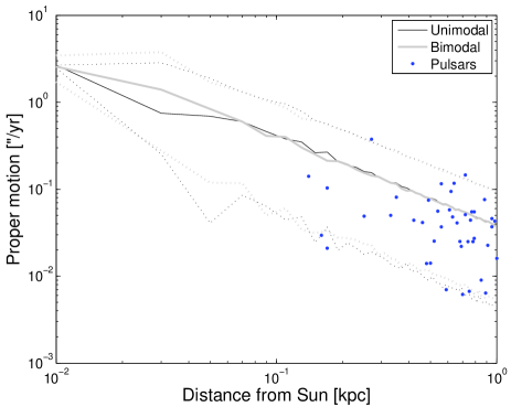
I note that the largest total proper motion in Table 4 (i.e., bimodal initial velocity distribution) is $4.6^{\prime\prime}$ yr^-1, and that $\sim 170N_{9}$ NSs are expected to have proper motion in excess of $1^{\prime\prime}$ yr^-1. In Table 5, the largest proper motion is $3.3^{\prime\prime}$ yr^-1, and about $240N_{9}$ NSs are expected to have proper motion in excess of $1^{\prime\prime}$ yr^-1.

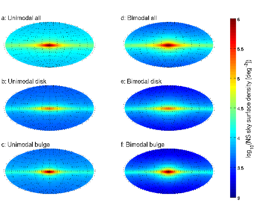
In Fig. 10a–f I show the sky surface density of NSs at the current epoch, for an observer located at the solar circle. Panels (a)–(c) are for the unimodal initial velocity distribution, while panels (d)–(f) are for the bimodal initial velocity distribution. Panels (a) and (d) show the distribution for all the NSs (i.e., disk- and bulge-born populations), panels (b) and (e) for the disk-born population, and panels (c) and (f) for the bulge-born population. The maps are shown in the Aitoff equal-area projection and Galactic coordinate system, where the Galactic center is at the center of each map. The surface densities are normalized assuming that there are $4\times 10^{8}$ disk-born NSs, and $6\times 10^{8}$ bulge-born NSs.

At the positions with the lowest surface density of NSs, the Poisson errors due to the limited statistics are smaller than about $10\%$. I find that the minimum surface density is attained at the direction of the Galactic poles, and is about $3900N_{9}$ deg^-2 and $8100N_{9}$ deg^-2 for the unimodal and bimodal initial velocity distributions, respectively. The maximum surface density is at the direction of the Galactic center and it is about $1.4\times 10^{6}N_{9}$ deg^-2 and $1.1\times 10^{6}N_{9}$ deg^-2, for the unimodal and bimodal initial velocity distributions, respectively. I note that the differences between the sky surface densities resulting from the two initial velocity distributions, are as large as about $65\%$.

7. Summary

The Milky Way’s NSs content, and in particular the NS space and velocity distributions are important for searching nearby isolated old NSs, and studying any ongoing activity from such objects. As a tool for such studies, I present a mock catalogue of simulated isolated old NSs spatial positions and velocities, at the current epoch.

The catalogue were constructed by integrating the equations of motion of simulated NSs in the Galactic potential. The simulations include two populations of NSs, one in which the NSs were born in the Galactic bulge about 12 Gyr ago, and the second population in which NSs are being born at the Galactic disk at a constant rate, starting 12 Gyr ago. The combined NS population assumes that $60\%$ of the NSs originated in the bulge and the rest in the disk. Although we do not know what is the exact number of Galactic NSs, and what was their position-dependent birth rate, these two populations provide a wide range of initial conditions.

I generated two catalogue of simulated NSs. Each catalog contains $3\times 10^{6}$ objects. The two catalogue utilize different initial velocity distributions of NSs. One catalog (Table 2) uses the initial velocity distribution of Arzoumanian et al. (2002), while the other (Table 3) uses the initial velocity distribution of Faucher-Giguère & Kaspi (2006). Also derived are catalogue of simulated NS positions and proper motions with respect to an observer found at the solar circle (tables 4 and 5).

The space distribution at the current epoch obtained by the two initial velocity distributions implemented here, are somewhat different. For example, I find that the resulting sky surface density, based on the two different initial velocity distributions, differs by up to $65\%$. The main differences between the two velocity distributions are in the low- and high-tails of the NSs velocity distribution (see Fig. 1).

Table 7Comparison with previous works

$\rho/N_{9}$	$Z_{1/2}$	mode$(p[v])$	Reference
pc-3	kpc	km s-1
$2.4\times 10^{-4}$	0.42	240	This Work (disk$+$bulge) A2002
$4.0\times 10^{-4}$	0.20	200	This Work (disk$+$bulge) FK2006
$1.4\times 10^{-3}$	0.20		Paczynski (1990)
$7.5\times 10^{-4}$	0.27	43	Blaes & Madau (1993)
$5.3\times 10^{-4}$	0.50	69	Madau & Blaes (1994)
$4\times 10^{-4}$		140	Perna et al. (2003)
$5\times 10^{-4}$	0.4		Popov et al. (2005)

Note. — The density, $\rho$, at the solar neighborhood is calculated assuming there are $10^{9}$ NSs in the Galaxy. $Z_{1/2}$ is the height above the Galactic plane, in which the NS density drops to $1/2$ its value on the Galactic plane, calculated at the solar circle. The density from Madau & Blaes (1994) is calculated assuming that diffusion operats for 5 Gyr (see §3). The initial velocity distribution used by Paczynski (1990), Blaes & Madau (1993), and Madau & Blaes (1994) is from Narayan & Ostriker (1990). The initial velocity distribution in Perna et al. (2003) is from Cordes & Chernoff (1998).

The space and velocity distributions of Galactic NSs were estimated by several past works. In Table 7, I compare some of the basic results of the simulations presented here (e.g., local density of NSs; scale height), with the ones obtained by previous efforts.

References

- Agüeros et al. (2006) Agüeros, M. A., et al. 2006, AJ, 131, 1740
- Arnett et al. (1989) Arnett, W. D., Schramm, D. N., & Truran, J. W. 1989, ApJL, 339, L25
- Arons & Lea (1976) Arons, J., & Lea, S. M. 1976, ApJ, 207, 914
- Arons & Lea (1980) Arons, J., & Lea, S. M. 1980, ApJ, 235, 1016
- Arzoumanian et al. (2002) Arzoumanian, Z., Chernoff, D. F., & Cordes, J. M. 2002, ApJ, 568, 289
- Aumer & Binney (2009) Aumer, M., & Binney, J. J. 2009, MNRAS in press (arXiv:0905.2512)
- Ballero et al. (2007) Ballero, S. K., Matteucci, F., Origlia, L., & Rich, R. M. 2007, A&A, 467, 123
- Barbanis & Woltjer (1967) Barbanis, B., & Woltjer, L. 1967, ApJ, 150, 461
- Binney & Tremaine (1987) Binney, J., & Tremaine, S. 1987, Galactic dynamics – Princeton, NJ, Princeton University Press, 1987, 747
- Blaauw (1961) Blaauw, A. 1961, Bull. Astron. Inst. Netherlands, 15, 265
- Blaes & Rajagopal (1991) Blaes, O., & Rajagopal, M. 1991, ApJ, 381, 210
- Blaes & Madau (1993) Blaes, O., & Madau, P. 1993, ApJ, 403, 690
- Bondi & Hoyle (1944) Bondi, H., & Hoyle, F. 1944, MNRAS, 104, 273
- Bower et al. (2007) Bower, G. C., Saul, D., Bloom, J. S., Bolatto, A., Filippenko, A. V., Foley, R. J., & Perley, D. 2007, ApJ, 666, 346
- Carlberg & Sellwood (1985) Carlberg, R. G., & Sellwood, J. A. 1985, ApJ, 292, 79
- Colpi et al. (1998) Colpi, M., Turolla, R., Zane, S., & Treves, A. 1998, ApJ, 501, 252
- Cordes & Chernoff (1998) Cordes, J. M., & Chernoff, D. F. 1998, ApJ, 505, 315
- Diehl et al. (2006) Diehl, R., et al. 2006, Nature, 439, 45
- Eisenhauer et al. (2005) Eisenhauer, F., et al. 2005, ApJ, 628, 246
- Faucher-Giguère & Kaspi (2006) Faucher-Giguère, C.-A., & Kaspi, V. M. 2006, ApJ, 643, 332
- Ferreras et al. (2003) Ferreras, I., Wyse, R. F. G., & Silk, J. 2003, MNRAS, 345, 1381
- Frei et al. (1992) Frei, Z., Huang, X., & Paczynski, B. 1992, ApJ, 384, 105
- Gal-Yam et al. (2006) Gal-Yam, A., et al. 2006, ApJ, 639, 331
- Ghez et al. (1998) Ghez, A. M., Klein, B. L., Morris, M., & Becklin, E. E. 1998, ApJ, 509, 678
- Ghez et al. (2008) Ghez, A. M., et al. 2008, ApJ, 689, 1044
- Haberl et al. (1998) Haberl, F., Motch, C., & Pietsch, W. 1998, Astronomische Nachrichten, 319, 97
- Hansen & Phinney (1997) Hansen, B. M. S., & Phinney, E. S. 1997, MNRAS, 291, 569
- Hartmann et al. (1990) Hartmann, D., Woosley, S. E., & Epstein, R. I. 1990, ApJ, 348, 625
- Hindmarsh (1983) Hindmarsh, A. C., 1983, ODEPACK, A systematized Collection of ODE Solvers, in Scientific Computing, R. S. Stepleman et al. (eds.), North-Holland, Amsterdam, 1983 (vol. 1 of IMACS Transactions of Scientific Computation), pp. 55-64.
- Hobbs et al. (2005) Hobbs, G., Lorimer, D. R., Lyne, A. G., & Kramer, M. 2005, MNRAS, 360, 974
- Jenkins & Binney (1990) Jenkins, A., & Binney, J. 1990, MNRAS, 245, 305
- Kamahori & Fujimoto (1987) Kamahori, H., & Fujimoto, M. 1987, PASJ, 39, 201
- Kamahori & Fujimoto (1986) Kamahori, H., & Fujimoto, M. 1986, PASJ, 38, 77
- Kasliwal et al. (2008) Kasliwal, M. M., et al. 2008, ApJ, 678, 1127
- Keane & Kramer (2008) Keane, E. F., & Kramer, M. 2008, MNRAS, 391, 2009
- Kida et al. (2008) Kida, S., et al. 2008, New Astronomy, 13, 519
- Klypin et al. (2002) Klypin, A., Zhao, H., & Somerville, R. S. 2002, ApJ, 573, 597
- Lai et al. (2006) Lai, D., Wang, C., & Han, J. 2006, Chinese Journal of Astronomy and Astrophysics Supplement, 6, 020000
- Levinson et al. (2002) Levinson, A., Ofek, E. O., Waxman, E., & Gal-Yam, A. 2002, ApJ, 576, 923
- Livio et al. (1998) Livio, M., Xu, C., & Frank, J. 1998, ApJ, 492, 298
- Madau & Blaes (1994) Madau, P., & Blaes, O. 1994, ApJ, 423, 748
- Manchester et al. (2005) Manchester, R. N., Hobbs, G. B., Teoh, A., & Hobbs, M. 2005, AJ, 129, 1993
- Maoz et al. (1997) Maoz, D., Ofek, E. O., & Shemi, A. 1997, MNRAS, 287, 293
- Matsumura et al. (2007) Matsumura, N., et al. 2007, AJ, 133, 1441
- Mazets et al. (1980) Mazets, E. P., Golenetskij, S. V., Aptecar, R. L., Guryan, Y. A., & Ilinskij, V. N. 1980, Soviet Astronomy Letters, 6, 318
- Meegan et al. (1992) Meegan, C. A., Fishman, G. J., Wilson, R. B., Horack, J. M., Brock, M. N., Paciesas, W. S., Pendleton, G. N., & Kouveliotou, C. 1992, Nature, 355, 143
- Metzger et al. (1997) Metzger, M. R., Djorgovski, S. G., Kulkarni, S. R., Steidel, C. C., Adelberger, K. L., Frail, D. A., Costa, E., & Frontera, F. 1997, Nature, 387, 878
- Minniti & Zoccali (2008) Minniti, D., & Zoccali, M. 2008, IAU Symposium, 245, 323
- Miyamoto & Nagai (1975) Miyamoto, M., & Nagai, R. 1975, PASJ, 27, 533
- Motch et al. (1997) Motch, C., Guillout, P., Haberl, F., Pakull, M., Pietsch, W., & Reinsch, K. 1997, A&A, 318, 111
- Narayan & Ostriker (1990) Narayan, R., & Ostriker, J. P. 1990, ApJ, 352, 222
- Neuhäuser & Trümper (1999) Neuhäuser, R., & Trümper, J. E. 1999, A&A, 343, 151
- Niinuma et al. (2007) Niinuma, K., et al. 2007, ApJL, 657, L37
- Noh & Scalo (1990) Noh, H.-R., & Scalo, J. 1990, ApJ, 352, 605
- Nordström et al. (2004) Nordström, B., et al. 2004, A&A, 418, 989
- Ofek (2007) Ofek, E. O. 2007, ApJ, 659, 339
- Ofek (2009) Ofek, E. O., Breslauer, B., Gal-Yam, A., Frail, D., Kasliwal, M. M., Kulkarni, S. R., 2009, ApJ submitted
- Ostriker et al. (1970) Ostriker, J. P., Rees, M. J., & Silk, J. 1970, ApL, 6, 179
- Paczynski (1990) Paczynski, B. 1990, ApJ, 348, 485
- Perna et al. (2003) Perna, R., Narayan, R., Rybicki, G., Stella, L., & Treves, A. 2003, ApJ, 594, 936
- Popov & Prokhorov (2000) Popov, S. B., & Prokhorov, M. E. 2000, A&A, 357, 164
- Popov et al. (2000) Popov, S. B., Colpi, M., Prokhorov, M. E., Treves, A., & Turolla, R. 2000, ApJL, 544, L53
- Popov et al. (2005) Popov, S. B., Turolla, R., Prokhorov, M. E., Colpi, M., & Treves, A. 2005, Ap&SS, 299, 117
- Posselt et al. (2008) Posselt, B., Popov, S. B., Haberl, F., Trümper, J., Turolla, R., & Neuhäuser, R. 2008, A&A, 482, 617
- Prokhorov & Postnov (1994) Prokhorov, M. E., & Postnov, K. A. 1994, A&A, 286, 437
- Quillen & Garnett (2001) Quillen, A. C., & Garnett, D. R. 2001, Galaxy Disks and Disk Galaxies, 230, 87
- Rocha-Pinto et al. (2000) Rocha-Pinto, H. J., Scalo, J., Maciel, W. J., & Flynn, C. 2000, ApJL, 531, L115
- Rutledge et al. (2003) Rutledge, R. E., Fox, D. W., Bogosavljevic, M., & Mahabal, A. 2003, ApJ, 598, 458
- Salpeter (1955) Salpeter, E. E. 1955, ApJ, 121, 161
- Seidelmann (1992) Seidelmann, P. K. 1992, Explanatory Supplement to the Astronomical Almanac, by P. Kenneth Seidelmann. Published by University Science Books, ISBN 0-935702-68-7, 752pp, 1992.
- Shvartsman (1971) Shvartsman, V. G. 1971, Soviet Astronomy, 14, 662
- Toropina et al. (2001) Toropina, O. D., Romanova, M. M., Toropin, Y. M., & Lovelace, R. V. E. 2001, ApJ, 561, 964
- Toropina et al. (2003) Toropina, O. D., Romanova, M. M., Toropin, Y. M., & Lovelace, R. V. E. 2003, ApJ, 593, 472
- Toropina et al. (2005) Toropina, O. D., Romanova, M. M., Toropin, Y. M., & Lovelace, R. V. E. 2005, Memorie della Societa Astronomica Italiana, 76, 508
- Treves & Colpi (1991) Treves, A., & Colpi, M. 1991, A&A, 241, 107
- Treves et al. (2001) Treves, A., Popov, S. B., Colpi, M., Prokhorov, M. E., & Turolla, R. 2001, X-ray Astronomy 2000, 234, 225
- Tully (1988) Tully, R. 1988, Nearby Galaxies Catalog (Cambrideg University Press)
- van Paradijs et al. (1997) van Paradijs, J., et al. 1997, Nature, 386, 686
- Voges et al. (1999) Voges, W., et al. 1999, A&A, 349, 389
- Wielen (1977) Wielen, R. 1977, A&A, 60, 263
- Yusifov & Küçük (2004) Yusifov, I., Küçük, I. 2004, A&A, 422, 545
- Zou et al. (2005) Zou, W. Z., Hobbs, G., Wang, N., Manchester, R. N., Wu, X. J., & Wang, H. X. 2005, MNRAS, 362, 1189