Mechanisms of jet formation on the giant planets

1 Introduction

Among the most striking features of the giant planets are the alternating zonal jets. As shown in Fig. 1, Jupiter and Saturn have prograde equatorial jets (superrotation) that peak at $\mathop{\sim}\!100\,\mathrm{m\,s^{-1}}$ and $\mathop{\sim}\!200$–$400\,\mathrm{m\,s^{-1}}$, depending on the vertical level considered. Uranus and Neptune have retrograde equatorial jets (subrotation) that peak at $\mathop{\sim}\!100\,\mathrm{m\,s^{-1}}$ and $\mathop{\sim}\!150$–$400\,\mathrm{m\,s^{-1}}$. Jupiter and Saturn have multiple off-equatorial jets in each hemisphere; Uranus and Neptune have only a single off-equatorial jet in each hemisphere. Despite decades of study with a variety of flow models, it has remained obscure how these different flow configurations come about (Vasavada and Showman 2005).

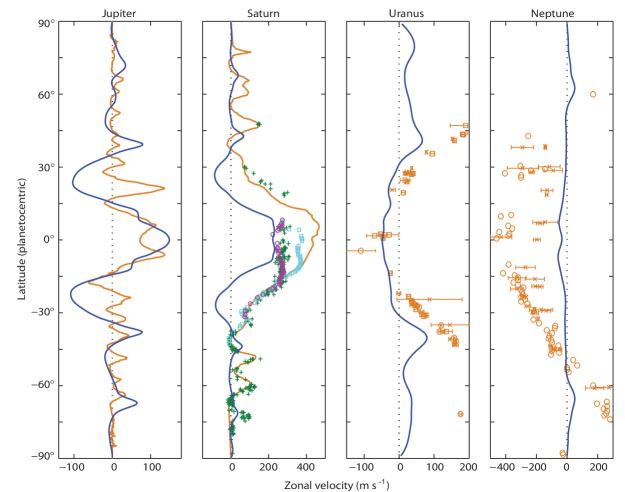
Figure 1: Mean zonal velocities in the upper atmosphere of the giant planets from observations and simulations. Jupiter: observations from the Cassini spacecraft (Porco et al. 2003) (orange line), and in simulation at $0.75$ bar (dark blue line). Saturn: observations from the Voyager spacecraft (orange line), from the Hubble Space Telescope (HST) (Sanchez-Lavega et al. 2003) (green crosses), from the Cassini spacecraft at $\mathop{\sim}\!0.06$ bar (magenta circles) and at $\mathop{\sim}\!0.7$ bar (light blue squares) (Sanchez-Lavega et al. 2007), and in simulation at $0.1$ bar (dark blue line). Uranus: observations from the Voyager spacecraft (orange circles), HST (orange crosses) (Hammel et al. 2001), the Keck telescope (orange squares) (Hammel et al. 2005), and in simulation at $25.0$ mbar (dark blue line). Neptune: observations from the Voyager spacecraft (orange circles) and from HST (orange crosses) (Sromovsky et al. 2001), and in simulation at $25.0$ mbar (dark blue line). Differences between the statistically identical northern and southern hemispheres in the simulations are indicative of the sampling variability of the averages.

Existing models posit as the driver of the flow either the differential radiative heating of the upper atmosphere (e.g., Williams 1979, 2003b) or the intrinsic heat fluxes emanating from the deep interior (e.g., Busse 1976; Heimpel et al. 2005; Aurnou et al. 2007; Chan and Mayr 2008; Kaspi et al. 2009). However, none of these models can account for the existence of equatorial superrotation on Jupiter and Saturn and equatorial subrotation on Uranus and Neptune with radiative heating, intrinsic heat fluxes, and other physical parameters consistent with observations.

For example, deep-flow models that posit intrinsic heat fluxes as the sole driver of the flow can generate equatorial superrotation, but they use heat fluxes more than $10^{6}$ times larger than those observed (e.g., Heimpel and Aurnou 2007). They generate equatorial subrotation only with intrinsic heat fluxes even stronger than those for which they generate superrotation (Aurnou et al. 2007), although the intrinsic heat fluxes on the subrotating planets (Uranus and Neptune) are weaker than those on the superrotating planets (Jupiter and Saturn). The relevance of such deep-flow models is further called into question by the eddy angular momentum fluxes they imply. Their meridional eddy fluxes of angular momentum per unit volume (taking density variations into account) have a barotropic structure: they extend roughly along cylinders concentric with the planet’s spin axis over the entire depth of the fluid, typically to pressures of order $10^{6}$ bar (e.g., Kaspi et al. 2009, their Fig. 10). But the eddy angular momentum fluxes inferred from tracking cloud features in Jupiter’s and Saturn’s upper tropospheres indicate that the mean conversion rate from eddy to mean-flow kinetic energy is of order $10^{-5}\,\mathrm{W\ m^{-3}}$ (Ingersoll et al. 1981; Salyk et al. 2006; Del Genio et al. 2007). If the observed upper-tropospheric eddy fluxes of angular momentum per unit volume extended unabatedly over a layer of 50 km thickness (e.g., from about 0.3 to 2.5 bar pressure on Jupiter, or from about 0.3 to 0.9 bar pressure on Saturn), and if vertical zonal flow variations over this layer are not dramatic, the total energy conversion rate would be about $0.5\,\mathrm{W\,m^{-2}}$. This is already $\mathop{\sim}\!4\%$ of the total energy uptake of the atmosphere from intrinsic heat fluxes and absorption of solar radiation for Jupiter, or $\mathop{\sim}\!11\%$ for Saturn. But the limited thermodynamic efficiency of atmospheres allows only a fraction of the total atmospheric energy uptake to be used to generate eddy kinetic energy (Lorenz 1955; Peixoto and Oort 1992). The observations of Jupiter and Saturn therefore imply that eddy angular momentum fluxes cannot extend unabatedly over great depths and must have a baroclinic structure. Barotropic eddy angular momentum fluxes that extend to depths of order $10^{6}$ bar, with upper-atmospheric fluxes of similar scale and magnitude as those observed, are only possible in deep-flow models if the driving heat fluxes are several orders of magnitude greater than observed.

Similarly, shallow-flow models that posit differential radiative heating as the driver of the flow can generate equatorial superrotation, but they require artifices such as additional equatorial heat or wave sources that have no clear physical interpretation (e.g., Williams 2003b, a; Yamazaki et al. 2005; Lian and Showman 2008). It is unclear in those and other shallow-flow models (e.g., Scott and Polvani 2008) what physical characteristics distinguish the superrotating planets from the subrotating planets.

In Schneider and Liu (2009) (SL09 hereafter), we postulated that prograde equatorial jets on the giant planets occur when intrinsic heat fluxes are strong enough that Rossby waves generated convectively in the equatorial region transport angular momentum toward the equator. Multiple off-equatorial jets, by contrast, form as a result of baroclinic instability owing to the differential radiative heating of the upper atmosphere. We introduced a general circulation model (GCM) and demonstrated with it that the postulated mechanisms can account qualitatively for large-scale flow structures observed on Jupiter. Here we use simulations with essentially the same GCM, with closed energy and angular momentum balances that are consistent with observations, to demonstrate universal formation mechanisms of jets on all the giant planets. We show that the different flow configurations on the giant planets can be explained through consideration of the different roles played by intrinsic heat fluxes and solar radiation in generating atmospheric waves and instabilities.

Section 2 briefly describes the GCM. Section 3 shows simulation results for Jupiter, Saturn, Uranus, and Neptune. Section 4 discusses the formation mechanisms of the jets in the simulations and confirms the postulated mechanisms through control simulations. Section 5 discusses what the upper-atmospheric fluid dynamics, on which we focus, imply about flows at greater depth on the giant planets. Section 6 summarizes the conclusions and their relevance for available and possible future observations.

2 General circulation model

With current computational resources, it is not feasible to simulate flows deep in giant planet atmospheres, where radiative relaxation times are measured in centuries and millennia, while at the same time resolving the energy-containing eddies in the upper atmospheres. Therefore, we focus on flows in the upper atmospheres, using a GCM that solves the hydrostatic primitive equations for a dry ideal-gas atmosphere in a thin spherical shell. The model is essentially that introduced for Jupiter in SL09, but here we use it to also simulate Saturn, Uranus, and Neptune. Parameters such as the planetary rotation rate, gravitational acceleration, and material properties of the atmosphere in each simulation are those of the planet being simulated. The resolution in each simulation (T85 to T213 spectral resolution in the horizontal and 30 or 40 levels in the vertical) is sufficient to resolve baroclinic instability and the energy-containing eddies in the upper atmosphere. The GCM and the simulations are described in detail in the appendix, and Table 1 lists the parameters; here we only give a brief overview.

Table 1: Simulation Parameters

Parameter, symbol	Jupiter	Saturn	Uranus	Neptune
Planetary radius, $a$ $(10^{6}\,\mathrm{m})$	$69.86$	$57.32$	$25.27$	$24.55$
Planetary angular velocity, $\Omega$ $(10^{-4}\,\mathrm{s})$	$1.7587$	$1.6388$	$1.0124$	$1.0834$
Gravitational acceleration, $g$ $(\mathrm{m\,s^{-2}})$	$26.0$	$10.55$	$8.94$	$11.2$
Specific gas constant, $R$ $(\mathrm{J\,kg^{-1}\,K^{-1}})$	$3605.38$	$4016.4$	$3149.2$	$3197.7$
Adiabatic exponent, $\kappa$	$2/7$	$2/7$	$2/7$	$2/7$
Specific heat capacity, $c_{p}=R/\kappa$ $(10^{4}\,\mathrm{J\,kg^{-1}\,K^{-1}})$	$1.26$	$1.41$	$1.10$	$1.12$
Solar constant $F_{0}$ $(\mathrm{W\,m^{-2}})$	$50.7$	$14.9$	$3.71$	$1.52$
Intrinsic heat flux $(\mathrm{W\,m^{-2}})$	$5.7$	$2.01$	$0.042$	$0.433$
Bond albedo, $r_{\infty}$	$0.343$	$0.342$	$0.30$	$0.29$
Single-scattering albedo, $\tilde{\omega}$	$0.8$	$0.8$	$0.8$	$0.8$
Solar optical depth at 3 bar, $\tau_{s0}$	$3.0$	$3.0$	$3.0$	$3.0$
Thermal optical depth at 3 bar, $\tau_{l0}$	$80.0$	$120.0$	$60.0$	$40.0$
Drag coefficient, $k_{0}$ $(\mathrm{days}^{-1}=(86400\,\mathrm{s}^{-1}))$	$1/100$	$1/100$	$1/100$	$1/100$
No-drag latitude, $\phi_{0}$	$33^{\circ}$	$33^{\circ}$	$33^{\circ}$	$33^{\circ}$
Horizontal spectral resolution	T213	T213	T85	T85
Vertical levels	30	30	40	40
Cut-off wavenumber for subgrid-scale dissipation	100	100	40	40
aGuillot (1999); bLodders and B. Fegley (1998); cLevine et al. (1977); dGierasch et al. (2000);
eGuillot (2005); fHanel et al. (1981); gHanel et al. (1983)

The GCM domain is a thin but three-dimensional spherical shell, which extends from the top of the atmosphere to an artificial lower boundary. The mean pressure at the lower boundary is $3$ bar in all our simulations, to minimize differences in arbitrary parameters among them. Insolation is imposed as perpetual equinox with no diurnal cycle at the top of the atmosphere. Absorption and scattering of solar radiation and absorption and emission of thermal radiation are represented in an idealized way that is consistent with observations where they are available (primarily for Jupiter). Where radiative and other parameters are not well constrained by observations or by knowledge of physical properties of the planets, we set them to be equal to the parameters for Jupiter, again to minimize differences in unconstrained parameters among the simulations. A dry convection scheme relaxes temperature profiles in statically unstable layers toward a convective profile with dry-adiabatic lapse rate, without transporting momentum in the vertical (see the appendix for details and for a discussion of this idealization).

At the lower boundary of the GCM, a temporally constant and spatially uniform intrinsic heat flux is imposed, with magnitude equal to the observed intrinsic heat fluxes ($5.70$, $2.01$, and $0.04$, and $0.43\,\mathrm{W\,m^{-2}}$ for Jupiter, Saturn, Uranus, and Neptune). (The heat flux in the Uranus simulation corresponds to an observational upper bound.) Linear (Rayleigh) drag retards the flow away from but not near the equator—a thin-shell representation of a magnetohydrodynamic (MHD) drag that acts at great depth (at pressures $\gtrsim 10^{5}$ bar), where the atmosphere becomes electrically conducting (Liu et al. 2008). Drag in a deep atmosphere affects the angular momentum balance averaged over cylinders concentric with the planet’s spin axis, so there is no effective drag on the flow in the upper atmosphere near the equator, in the region in which the cylinders do not intersect the layer of MHD drag at depth (SL09). Absent detailed knowledge of where and how the MHD drag acts and to rule out that differences among the simulations are caused by differences in the drag formulation, we chose the equatorial no-drag region to extend to $\phi_{0}=33^{\circ}$ latitude and the drag coefficient outside this region to be the same in all simulations. Section 4d discusses the effect of this drag formulation on our simulation results, and section 5 and the appendix provide further justification for it.

We show simulation results from statistically steady states, which were reached after long spin-up periods; see the appendix for details. The northern and southern hemispheres in the simulations are statistically identical, so differences between the hemispheres in figures showing long-term averages are indicative of the sampling variability of the averages.

3 Simulation results

a Upper-atmospheric zonal flow

Figure 1 shows the simulated mean zonal velocities near the levels at which cloud features from which the observed flows are inferred are suspected to occur: in the Jupiter simulation at 0.75 bar, corresponding to the layer of ammonia ice clouds on the actual planet (Atreya et al. 1999); in the Saturn simulation at 0.1 bar, in a layer of tropospheric (e.g., ammonia) hazes (Sanchez-Lavega et al. 2007); in the Uranus and Neptune simulations at 25 mbar, near the top of the stratospheric layers in which hydrocarbons would condense and form hazes (Gibbard et al. 2003).

The simulations reproduce large-scale features of the observed flows in the upper atmosphere (Fig. 1). The Jupiter and Saturn simulations exhibit equatorial superrotation, the Uranus and Neptune simulations equatorial subrotation. The equatorial jet in the Jupiter simulation has similar strength ($\mathop{\sim}\!150\,\mathrm{m\,s^{-1}}$) and width as the observed jet. The equatorial jet in the Saturn simulation is stronger ($\mathop{\sim}\!230\,\mathrm{m\,s^{-1}}$) and slightly wider than that in the Jupiter simulation, but it is weaker and narrower than the observed jet at a corresponding level on Saturn. The Jupiter and Saturn simulations exhibit alternating off-equatorial jets; they are broader than the observed jets but of similar strength. Especially in the Saturn simulation, the retrograde jets (except for the first retrograde jet off the equator) are broad and weak with speeds less than $10\,\mathrm{m\,s^{-1}}$. They are more manifest as local minima of the zonal velocity than as actual retrograde jets. The Uranus and Neptune simulations exhibit a single off-equatorial jet in each hemisphere. The overall structure of the jets in the Uranus and Neptune simulations is roughly consistent with observations, but the equatorial jet in the Neptune simulation at the level shown ($\mathop{\sim}\!-40\,\mathrm{m\,s^{-1}}$) is considerably weaker than that observed. (However, the jet is stronger at higher levels in the simulation; see Fig. 5 below.)

In general, the prograde jets (or zonal velocity maxima) are sharper than the retrograde jets (or zonal velocity minima), consistent with the zonal velocity maxima being barotropically more stable (Rhines 1994). Indeed, meridional gradients of both absolute vorticity and quasigeostrophic potential vorticity at the levels at which the zonal velocities are shown in Fig. 1 are small near zonal velocity minima and are reversed near some of them (Fig. 2). (The quasigeostrophic potential vorticity is not shown for the Jupiter simulation because the stratification at the corresponding level is nearly statically neutral, so that potential vorticity is not well defined; see Fig. 5 below.) The changing magnitude of the vorticity gradients between zonal velocity maxima and minima gives rise to a staircase pattern of absolute vorticity and potential vorticity as a function of latitude (McIntyre 1982; Dritschel and McIntyre 2008). Absolute vorticity gradients can reach about $-2\beta$, particularly in higher latitudes in the flanks of the minima; quasigeostrophic potential vorticity gradients are also reversed near some of the zonal velocity minima, particularly in the Uranus and Neptune simulations, but they do not reach as strongly negative values as the absolute vorticity gradients. These features are roughly consistent with observations of Jupiter and Saturn (Ingersoll et al. 1981; Read et al. 2006), but quasigeostrophic potential vorticity gradients may be more strongly negative on Saturn than they are in our simulation (Read et al. 2009). The vorticity profiles indicate that barotropic instability limits the sharpening of the retrograde jets, though not to the degree that the statistically steady states of the flows would satisfy sufficient conditions for linear barotropic stability for unforced and non-dissipative flows. (There is no reason that such sufficient conditions ought to be satisfied in forced-dissipative flows.)

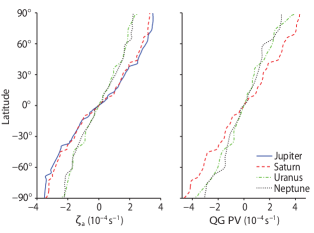
Figure 2: Mean absolute vorticity (left) and quasigeostrophic potential vorticity (right) in the simulations, evaluated at the same levels at which the zonal velocities are shown in Fig. 1. The quasigeostrophic potential vorticity is calculated analogously to Read et al. (2009). It is not shown for the Jupiter simulation because the stratification at the corresponding level is nearly statically neutral (cf. Fig. 5 below), so potential vorticity is not well defined.

The jets are not only evident in long-term averages but also in instantaneous flow fields. The instantaneous zonal velocity and vorticity fields show the jets as well as large-scale jet undulations, waves, and coherent vortices (Fig. 3). In the equatorial region in the Jupiter and Saturn simulations, the waves are organized into large wave packets (Fig. 3, left column). Animations of the flow fields show that the wave packets exhibit westward group propagation, as expected for long equatorial Rossby waves (Matsuno 1966; Gill 1982, chapter 11). In the vorticity fields (Fig. 3, right column), coherent vortices are seen in latitude regions with nearly homogenized absolute vorticity or potential vorticity, that is, in regions with large negative curvature of the zonal flow with latitude (cf. Fig. 2).

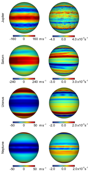
Figure 3: Zonal velocity (left column) and relative vorticity (right column) at one instant in the statistically steady state of the simulations. The levels at which the flow fields are shown are the same as in Fig. 1. The equatorial Rossby waves (organized into large wave packets) that are responsible for the generation of the equatorial superrotation are recognizable in the Jupiter and Saturn simulations. Coherent vortices are clearly seen in the Jupiter and Uranus simulations. Animations of the flow fields are available at http://www.gps.caltech.edu/~tapio/pubs.html.

b High-latitude coherent vortices and waves on jets

In high latitudes in the Jupiter and Saturn simulations, very large coherent vortices ($20^{\circ}\times 10^{\circ}$ longitude$\times$latitude) form spontaneously (Fig. 4). They extend all the way to the bottom of the domain, with the magnitude of the vorticity decreasing weakly with depth: the peak vorticity at the bottom of the domain is about $80\%$ of its maximum value in the column.

The large coherent vortices are cyclonic, with typical vorticities of magnitude $\mathop{\sim}\!2\times 10^{-5}\ \mathrm{s^{-1}}$. They are advected by the flow in their environment and have a local temperature minimum at the center ($\mathop{\sim}\!10\,\mathrm{K}$ lower temperature than the environment). These cyclonic vortices are long-lived, with life-spans apparently determined by the radiative timescale (the timescale on which eddies can modify the mean flow). In the Jupiter simulation with an atmosphere of $3$ bar thickness, the radiative timescale is $\mathop{\sim}\!10$ Earth years; it is $\mathop{\sim}\!50$ Earth years in the Saturn simulation. Since the radiative timescale increases with pressure, it is longer for deeper atmospheres, which might explain why the observed coherent vortices such as the Great Red Spot on Jupiter are so long-lived.

Coherent vortices preferentially exist in regions where absolute vorticity or potential vorticity gradients vanish, as they can then arise spontaneously in barotropic or quasigeostrophic flows and remain stable (e.g., McWilliams 1984; Marcus 1988, 1993). Since the planetary vorticity gradient vanishes at the poles, formation of coherent vortices in high latitudes may require less vorticity mixing in the environment than it does at lower latitudes. Hence, the large coherent vortices in high latitudes may appear earlier in simulations. If the simulations were conducted for a (much) longer period and if numerical (subgrid-scale) dissipation could be further reduced, it is possible that large coherent vortices would also appear in lower latitudes, such as the latitude ($23^{\circ}$S planetocentric) of the Great Red Spot on Jupiter, which is embedded in an environment of small absolute vorticity and potential vorticity gradients (Ingersoll et al. 1981; Read et al. 2006).

The coherent polar vortices in our simulations are contained in the polar cap bounded by the highest-latitude prograde jet. These polar jets exhibit large-scale undulations, as do other jets (cf. Fig. 3). In the Saturn simulation, for example, the prograde polar jet at $68^{\circ}$N exhibits a wavenumber-8 or 9 undulation (Fig. 4), with a zonal phase velocity of $-24\,\mathrm{m\,s^{-1}}$. This is retrograde, and retrograde relative to the mean flow, consistent with the undulation being a Rossby wave. The undulation is reminiscent of the nearly stationary wavenumber-6 pattern (“polar hexagon”) observed in Saturn’s polar atmosphere at $76^{\circ}$N planetocentric latitude (Godfrey 1988; Allison et al. 1990; Fletcher et al. 2008). Indeed, with a smaller drag coefficient that leads to a slightly stronger polar jet (see section 4d), we also obtain a wavenumber-6 pattern on the polar jet in our simulations; we will describe this in greater detail elsewhere.

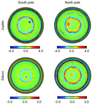
Figure 4: Relative vorticity ($10^{-5}\,\mathrm{s^{-1}}$) in high latitudes at one instant in the statistically steady state of the Jupiter and Saturn simulations. Left column: south polar projection; right column: north polar projection. The vorticity is shown at the same levels as the flow fields in Figs. 1 and 3 (0.75 and 0.1 bar, respectively).

c Vertical structure of zonal flow

The simulated flows in Figs. 1–4 were shown near the suspected levels of observed cloud features on the giant planets. However, the flows in the simulations vary in the vertical. The prograde equatorial jets in the Jupiter and Saturn simulations strengthen with depth (Fig. 5, left column). The corresponding vertical shear of the zonal flow ($\mathop{\sim}\!1$–$2\times 10^{-3}\,\mathrm{s^{-1}}$) is similar to that measured by the Galileo probe on Jupiter between 0.7 bar and 4 bar (Atkinson et al. 1998) and to that inferred from Cassini data for Saturn between 0.05 and 0.8 bar (Sanchez-Lavega et al. 2007; see also the zonal flow observations at different levels in Fig. 1). The retrograde equatorial jets in the Uranus and Neptune simulations are strongest in the stratosphere and weaken with depth, consistent with inferences drawn from gravity measurements with the Voyager 2 spacecraft (Hubbard et al. 1991). Away from the equator, prograde jets generally weaken with depth and retrograde jets strengthen slightly or do not vary much with depth.

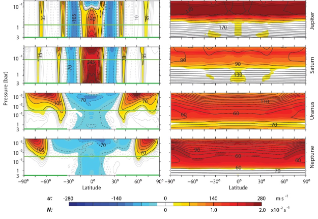
Figure 5: Mean flow fields in the latitude-pressure plane in the simulations. The left column shows zonal-flow profiles: Gray contours for zonal flow speeds between $5$ and $30\,\mathrm{m\,s^{-1}}$, with a contour interval of $5\,\mathrm{m\,s^{-1}}$; black contours for zonal flow speeds of $35\,\mathrm{m\,s^{-1}}$ or above, with a contour interval of of $35\,\mathrm{m\,s^{-1}}$. Solid contours and red tones for prograde flow and dashed contours and blue tones for retrograde flow. The right column shows temperature (contours, contour interval 10 K) and buoyancy frequency $N$ (colors). The thick green parts of the latitude axes in the left column mark the latitudes with nonzero drag. The thin green lines indicate the levels at which flow fields are shown in Figs. 1–4.

d Temperature structure

Consistent with thermal wind balance, temperatures increase equatorward along isobars where prograde jets weaken with depth or retrograde jets strengthen with depth, and they decrease equatorward where the opposite is true. Therefore, in the equatorial upper troposphere in the Jupiter and Saturn simulations, where the prograde jets strengthen with depth, temperatures decrease equatorward and have a minimum at the equator (Fig. 5, contours in right column). A similar equatorial temperature minimum is seen in observations of Jupiter and Saturn (Simon-Miller et al. 2006; Fletcher et al. 2007). The tropopause, recognizable as the level at which the vertical temperature lapse rate changes sign, in all simulations lies near $0.1$ bar, likewise as observed (Simon-Miller et al. 2006; Fletcher et al. 2007). Below the tropopause, temperatures increase with depth. In the Jupiter, Saturn, and Neptune simulations, the atmosphere is close to statically neutrally stratified below the statically stable layer near the tropopause because of vigorous convection driven by intrinsic heat fluxes. In the Uranus simulation, the entire atmosphere is stably stratified (or close to it) because convection and intrinsic heat fluxes are weak (Fig. 5, colors in right column).

In the Jupiter simulation, the equator-to-pole contrast in the brightness temperature of thermal radiation is 10 K, which is similar to albeit larger than the observed brightness temperature contrast or the observed temperature contrast near the emission level (Ingersoll et al. 1976; Ingersoll 1990; Ingersoll et al. 2004; Simon-Miller et al. 2006). In the Saturn simulation, the equator-to-pole brightness temperature contrast is 7 K, consistent with observations (Ingersoll 1990; Fletcher et al. 2007). In the Uranus and Neptune simulations, the equator-to-pole brightness temperature contrasts are 8 K and 2 K, respectively, consistent with observations (Ingersoll 1990). That is, meridional enthalpy transport in all simulations substantially reduces the (much greater) radiative-convective equilibrium temperature contrasts near the emission levels. (The emission levels lie between about $0.3$ and $0.5$ bar in our simulations, and radiative-convective equilibrium temperature contrasts there vary between 20 K for Neptune and 35 K for Uranus.) It does not appear necessary to invoke meridional mixing deep in the atmosphere to account for the smallness of the observed brightness temperature contrasts (cf. Ingersoll 1976; Ingersoll and Porco 1978).

However, although temperature contrasts at the emission level are generally small, equator-to-pole temperature contrasts at higher or lower levels of the simulated atmospheres differ, and the same is likely true for the actual planets. For example, while temperature contrasts near the emission level in the Jupiter simulation are small, they are greater at lower levels where temperatures are greater (Fig. 6a). Because the atmosphere is close to statically neutrally stratified below the upper troposphere, entropy (potential temperature) there is constant in the vertical. [More generally, entropy is constant along angular momentum surfaces, to achieve a state of neutrality with respect to slantwise convection; see Emanuel (1983) and Thorpe and Rotunno (1989).] Hence, the meridional potential temperature distribution at lower levels is the same as that near the top of the neutrally stratified layer, except near the equator where the atmosphere has a weak positive static stability (Fig. 6b). But this implies that meridional temperature gradients off the equator increase with pressure, as temperature $T$ and potential temperature $\theta$ are related by $T=\theta(p/p_{0})^{\kappa}$, where $p$ is pressure and $p_{0}$ a constant reference pressure. In particular, the signatures of the prograde off-equatorial jets weakening with depth (enhanced meridional temperature gradients) and of the retrograde off-equatorial jets strengthening slightly or not varying with depth (reduced or vanishing meridional temperature gradients) are visible at all levels (Figs. 6a and b). There are no observations of entropy or temperature distributions below the upper troposphere for the giant planets, but we expect them to behave similarly as in our simulations, for the reasons discussed in section 5c below.

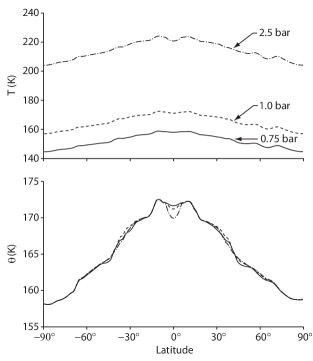
Figure 6: Temperature (a) and potential temperature (b) at the $0.75$-bar (solid), $1.0$-bar (dashed), and $2.5$-bar (dash-dotted) levels in Jupiter simulation. The potential temperature $\theta=T(p_{0}/p)^{\kappa}$ is evaluated with the reference pressure $p_{0}=1$ bar.

4 Mechanisms of jet formation

Why are the flow and temperature structures in the giant planet simulations so different? The fundamental reason lies in the different strengths of the differential radiative heating and the intrinsic heat flux, and in the different ways in which the two can lead to the generation of the eddies that maintain the jets. Eddies in rapidly rotating atmospheres generally transport angular momentum from their dissipation (breaking) region into their generation region (Held 1975; Andrews and McIntyre 1976, 1978; Rhines 1994; Held 2000; Vallis 2006, chapter 12). If they are preferentially generated in prograde jets, they lead to angular momentum transport from retrograde into prograde jets, which can maintain the jets against dissipation (e.g., Vallis 2006; O’Gorman and Schneider 2008). Such angular momentum transport from retrograde into prograde jets has indeed been observed on Jupiter and Saturn (Ingersoll et al. 1981; Salyk et al. 2006; Del Genio et al. 2007). A central question is, then, what kind of eddies can give rise to the angular momentum transport required to spin up and maintain the jets? We have addressed this question more formally and in greater detail in SL09. Here we summarize some results from that earlier paper and expand on some that are important for understanding the simulations presented in this paper.

a Off-equatorial jets

Away from the equator, the differential radiative heating of the upper atmospheres produces meridional temperature gradients, which are baroclinically unstable and lead to eddy generation. Eddy generation preferentially occurs in the troposphere in the baroclinically more unstable prograde jets with enhanced temperature gradients and enhanced prograde vertical shear (Fig. 5). It results in angular momentum transport from retrograde into prograde tropospheric jets (Fig. 7). This angular momentum transport maintains the off-equatorial tropospheric jets in the Jupiter and Saturn simulations against dissipation at depth. It has a baroclinic structure and, in the Jupiter and Saturn simulations, is in structure and magnitude consistent with observations (cf. Ingersoll et al. 1981; Salyk et al. 2006; Del Genio et al. 2007). The conversion rate of eddy to mean-flow kinetic energy is of order $10^{-5}\,\mathrm{W\,m^{-3}}$ in the upper tropospheres in the Jupiter and Saturn simulations—as observed. In the global mean, the conversion rates are $0.09\,\mathrm{W\,m^{-2}}$ and $0.026\,\mathrm{W\,m^{-2}}$ in the Jupiter and Saturn simulations, respectively, implying that the conversion rate in either simulation is about 0.6% of the total energy uptake of the atmosphere. Consistent with a baroclinic eddy generation mechanism, off-equatorial eddy angular momentum fluxes and jets disappear in a Jupiter control simulation in which baroclinic instability is suppressed by imposing insolation uniformly at the top of the atmosphere (SL09).

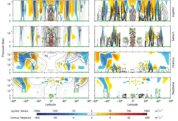
Figure 7: Mean zonal velocities, mass flux streamfunction (contours) and divergence $\mathop{\mathrm{div}}(\overline{u^{\prime}v^{\prime}}\,a\cos\phi)$ of meridional eddy angular momentum fluxes (colors) in the simulations. The left column shows zonal-flow profiles (contours as in Fig. 5) and eddy angular momentum flux divergence (colors). The right column shows the mass flux streamfunction (contours) and the same eddy angular momentum flux divergence as in the left column (colors). The contouring for the streamfunction is logarithmic: black contours from $\pm 1$ to $\pm 64\times 10^{8}\,\mathrm{kg\,s^{-1}}$; gray contours for absolute values greater than or equal to $128\times 10^{8}\,\mathrm{kg\,s^{-1}}$, with factors of 2 separating contour levels. (Black contours that would be within gray contours are not shown.) Solid contours for positive streamfunction values (counterclockwise rotation) and dashed contours for negative streamfunction values (clockwise rotation). Some streamfunction contours are truncated at the bottom of the plotting domain (3 bar) because they close at higher pressures (the pressure at the bottom of the GCM domain can locally exceed 3 bar). The contouring for the eddy angular momentum flux divergence is likewise logarithmic, with the scale shown in the colorbar. As in Fig. 5, the thick green parts of the latitude axes mark the latitudes with nonzero drag.

The off-equatorial jets in the Uranus and Neptune simulations are situated in the stratosphere and are broader than those in the Jupiter and Saturn simulations. They appear to be broader because only the longest waves generated at lower levels are able to reach the stratosphere (Charney and Drazin 1961). Indeed, the eddy angular momentum flux divergence at the stratospheric jet cores is much weaker than that at the tropospheric jet cores in the Jupiter and Saturn simulations (Fig. 7). It is not even of a consistent sign at all times but exhibits considerable low-frequency variability, as indicated by the differences between the statistically identical hemispheres in the long-term (1500-day) averages shown in Fig. 7. The jets become very weak below the tropopause and, particularly in the Uranus simulation, give way to a tropospheric zonal flow with smaller meridional scales (Fig. 5). The structure of the stratospheric jets implies that they interact only weakly with the drag at the lower boundary, so only weak eddy angular momentum flux divergence is necessary to maintain them. The jets are primarily a manifestation of the thermal structure and of the vertical shear of the zonal flow implied by it. The latter do not exhibit smaller-scale variations because smaller-scale eddy transports of angular momentum and heat in the stratosphere are weak.

b Equatorial superrotation

Near the equator, convection can penetrate into the upper troposphere and can generate Rossby waves if the intrinsic heat flux is strong enough to overcome the static stabilization of the atmosphere by the radiative heating from above. Fluctuations in convective heating are primarily balanced by vertical motion and, at the level of the convective outflows, by horizontal divergence of mass fluxes, as in the tropics of Earth’s atmosphere. That is, the dominant balance in the thermodynamic equation is the weak-temperature gradient (WTG) balance (Sobel et al. 2001),

$$\boldsymbol{\mathrm{\nabla}}_{h}\cdot\boldsymbol{\mathrm{v}}_{\chi}\approx\partial_{p}(Q/S).$$ (1)

Here, $\boldsymbol{\mathrm{v}}_{\chi}$ denotes the divergent horizontal flow component, $Q=D\theta/Dt$ the diabatic heating rate, and $S=-\partial_{p}\theta$ the static stability; the subscript $h$ on the differential operator $\boldsymbol{\mathrm{\nabla}}_{h}$ signifies horizontal derivative. As discussed in Sardeshmukh and Hoskins (1988), fluctuations in the horizontal divergence are a source of equatorial Rossby waves, and the fluctuating vorticity source

$$R^{\prime}=R-\bar{R},$$ (2a)

with

$$R=-\zeta_{a}(\boldsymbol{\mathrm{\nabla}}_{h}\cdot\boldsymbol{\mathrm{v}}_{\chi})-(\boldsymbol{\mathrm{v}}_{\chi}\cdot\boldsymbol{\mathrm{\nabla}}_{h})\zeta_{a},$$ (2b)

can be taken to be the Rossby wave source. (The overbar denotes the isobaric zonal and temporal mean and primes deviations therefrom.) Thus, fluctuations in convective heating lead to horizontal divergence fluctuations (1), which can generate equatorial Rossby waves through stretching of absolute vorticity $\zeta_{a}$ or advection of absolute vorticity by the divergent flow $\boldsymbol{\mathrm{v}}_{\chi}$ (2). Because the planetary vorticity vanishes at the equator, the Rossby wave source $R^{\prime}$ typically has largest amplitude just off the equator, but it does not necessarily vanish at the equator or where the absolute vorticity vanishes because absolute vorticity advection by the divergent flow may not vanish.

Equatorial Rossby waves, organized into large-scale wave packets, are recognizable in the Jupiter and Saturn simulations in Fig. 3. In the Jupiter simulation, the energy-containing zonal wavenumber is $\mathop{\sim}\!10$, corresponding to the wavenumber of the wave packet envelope. Waves with similar scales have also been observed on Jupiter (Allison et al. 1990). The retrograde tilt of the waves’ phase lines away from the equator, clearly seen in the Jupiter simulation (Fig. 3), indicates that they transport angular momentum toward the equator (cf. Peixoto and Oort 1992, chapter 11). This is generally to be expected for such convectively generated Rossby waves: they transport angular momentum toward the equatorial region because this is where they are preferentially generated. The Rossby wave source $R^{\prime}$ owing to horizontally divergent flow has largest amplitude in the equatorial region because only there will convective heating fluctuations necessarily lead to horizontal divergence fluctuations on large scales; away from the equator, the WTG approximation (1) of the thermodynamic equation does not hold. [See SL09 (their Fig. 5) for a demonstration that $R^{\prime}$ has largest amplitude near the equator.] The angular momentum transport toward the equatorial region by convectively generated Rossby waves leads to equatorial superrotation if it is sufficiently strong and drag on the zonal flow is sufficiently weak (SL09).

Convective Rossby wave generation near the equator is the key process responsible for superrotation in the Jupiter and Saturn simulations. In SL09, we demonstrated that without intrinsic heat fluxes and the convection they induce, a Jupiter simulation similar to the one here exhibits equatorial subrotation; the same is true for the Jupiter and Saturn simulations here. Therefore, we suggest convective Rossby wave generation is what causes the superrotating equatorial jets on Jupiter and Saturn.

When convective Rossby wave generation produces equatorial superrotation, it produces a jet whose half-width $L_{s}$ is similar to the scale of equatorial Rossby waves: the equatorial Rossby radius $L_{\beta}=\sqrt{c/\beta}$, with gravity wave speed $c$ and planetary vorticity gradient $\beta$. Vorticity mixing arguments give an estimate for the maximum strength of the equatorial jet (Rhines 1994, SL09): If the end state of vorticity mixing is a state in which the absolute vorticity is homogenized across the equatorial jet in each hemisphere separately, with a barotropically stable jump at the equator, and if the jet half-width $L_{s}$ is similar to the equatorial Rossby radius $L_{\beta}$, the jet speed at the equator will be

$$U\lesssim\frac{\beta L_{s}^{2}}{2}\sim\frac{c}{2}.$$ (3)

To the extent that this bound is attained (at the level of maximum equatorial jet speed), the jet speed increases quadratically with the jet width. This is roughly consistent with observations of Jupiter and Saturn (though the maximum equatorial jet speed on Saturn is not known for lack of observations deeper in the atmosphere). It is also roughly consistent with our simulations, although a state of homogenized absolute vorticity in the equatorial region of each hemisphere is not attained in the simulations. That is, the equatorial jet on Saturn may be stronger and wider than that on Jupiter because the gravity wave speed is larger.

The flow configurations in the Jupiter and Saturn simulations differ qualitatively from those in the Uranus and Neptune simulations because the relative strengths of baroclinic eddy generation away from the equator and convective Rossby wave generation near the equator differ. In the Uranus simulation, the intrinsic heat flux is negligible, the atmosphere is stably stratified, and there is no substantial convective Rossby wave source near the equator. Consequently, the equatorial eddy kinetic energy is weak, and the equatorial flow is retrograde.

In the Neptune simulation, the intrinsic heat flux is strong enough that convection penetrates into the upper troposphere. As in the other simulations, eddies can be generated by (a) baroclinic instability off the equator induced by differential solar heating, or (b) convective Rossby wave generation near the equator induced by the intrinsic heat flux. Eddies produced by these two mechanisms compete with each other in their contribution to the angular momentum transport to or from low latitudes. Off-equatorial baroclinic eddy generation implies angular momentum flux convergence in the off-equatorial generation regions and divergence in lower latitudes, and hence a tendency toward retrograde equatorial flow. Convective Rossby wave generation near the equator can lead to prograde equatorial flow, but in the Neptune simulation, the rms Rossby wave source $R^{\prime}$ in the equatorial region is much smaller than that in the Jupiter and Saturn simulations: the rms Rossby wave source $R^{\prime}$ in the upper troposphere near the equator is $\mathop{\sim}\!10^{-12}\,\mathrm{s^{-2}}$ for Neptune but $\mathop{\sim}\!10^{-10}\,\mathrm{s^{-2}}$ for Jupiter and Saturn. Convective Rossby wave generation and the associated angular momentum flux convergence near the equator appear to be too weak to overcome the angular momentum flux divergence in low latitudes that is caused by eddies generated baroclinically away from the equator. As a consequence, the equatorial flow is retrograde. This is corroborated by control simulations.

c Neptune control simulations

We investigated the relative roles of baroclinic eddy generation and convective Rossby wave generation on Neptune in two control simulations, one in which the convective Rossby wave source was enhanced and one in which the baroclinic eddy generation caused by differential solar heating was suppressed. Because angular momentum flux divergence in low latitudes owing to baroclinic eddy generation away from the equator can counteract any angular momentum flux convergence owing to convective Rossby wave generation, generation of equatorial superrotation in the Neptune simulation may require a stronger intrinsic heat flux or weaker differential solar heating.

Indeed, a control simulation with Neptune’s physical parameters but in which the convective Rossby wave source was enhanced by enhancing the intrinsic heat flux—setting it to Saturn’s $2.01\,\mathrm{W\ m^{-2}}$ in place of Neptune’s $0.433\,\mathrm{W\ m^{-2}}$—exhibits equatorial superrotation (Fig. 8, left column). Conversely, a control simulation in which baroclinic eddy generation was suppressed by imposing insolation uniformly at the top of the atmosphere (but keeping the global mean fixed) also exhibits equatorial superrotation (Fig. 8, right column). The prograde off-equatorial jets disappear with the suppression of baroclinicity.

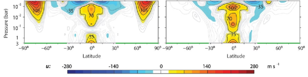
Figure 8: Mean zonal velocities in the latitude-pressure plane in Neptune control simulations. Contour intervals and colors as in Fig. 5. Left: simulation with Neptune’s physical parameters but Saturn’s intrinsic heat flux ($2.01\ \mathrm{W\ m^{-2}}$). Right: simulation with Neptune’s physical parameters but uniform insolation at the top of the atmosphere.

We suggest, then, that Uranus and Neptune exhibit equatorial subrotation because baroclinic eddy generation away from the equator is strong compared with convective Rossby wave generation near the equator. Interestingly, our simulations suggest that Neptune’s intrinsic heat flux only needs to be larger by an $O(1)$ factor for Neptune’s atmosphere to develop equatorial superrotation, implying that Neptune may have been superrotating earlier in its history, when intrinsic heat fluxes were stronger.

d Effect of drag formulation on simulated flows

One relatively unconstrained aspect of our simulations is the strength and functional form of the drag at the artificial lower boundary. We investigated the sensitivity of our results to the drag formulation by varying it in a few Jupiter simulations.

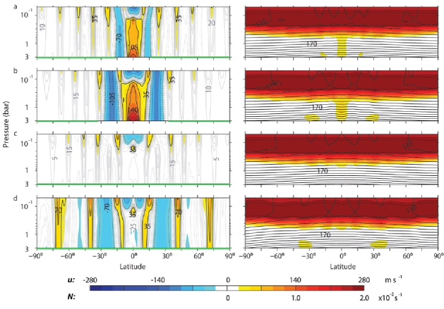
Figure 9: Mean flow fields in the latitude-pressure plane in Jupiter simulations with different drag formulations. The left column shows the zonal flow and the right column the temperature and buoyancy frequency, with the same plotting conventions and contour intervals as in Fig. 5. (a) No drag in the equatorial region up to $\phi_{0}=16^{\circ}$, and off-equatorial drag coefficient $k_{0}=1/(20\,\mathrm{days})$. (b) No drag in the equatorial region up to $\phi_{0}=33^{\circ}$, and off-equatorial drag coefficient $k_{0}=1/(10\,\mathrm{days})$. (c) Constant drag at all latitudes with drag coefficient $k_{0}=1/(10\,\mathrm{days})$. (d) Constant drag at all latitudes with drag coefficient $k_{0}=1/(100\,\mathrm{days})$.

The Jupiter simulation in SL09 had an equatorial no-drag region half as wide as that here (extending to $\phi_{0}=16^{\circ}$ latitude vs. $\phi_{0}=33^{\circ}$ here), in addition to having a larger drag coefficient off the equator [$k_{0}=1/(20\,\mathrm{days})$ vs. $k_{0}=1/(100\,\mathrm{days})$ here]. Mean flow fields from that earlier simulation are shown in Fig. 9a. The half-width of the prograde equatorial jet is $\mathop{\sim}\!5^{\circ}$ smaller than in the Jupiter simulation reported here (cf. Fig. 5). The adjacent strong retrograde jets appear to be confined to the no-drag region and hence do not extend as far poleward as in the simulation with the wider no-drag region. The off-equatorial jets are somewhat weaker and narrower—a result of the enhanced off-equatorial drag, consistent with theories and other simulations of geophysical turbulence (Smith et al. 2002; Danilov and Gurarie 2002). However, the width of the equatorial no-drag region does not primarily control the strength or width of the equatorial jet, as evidenced by the relatively moderate changes in the flow in low latitudes in response to the factor 2 change in the width of the no-drag region.

That the strength and width of off-equatorial jets depend on the drag coefficient is directly illustrated by simulations in which we increased the off-equatorial drag coefficient further [Fig. 9b, $k_{0}=1/(10\,\mathrm{days})$]. The off-equatorial jets become weaker and narrower as the drag coefficient is increased. However, if the same enhanced drag is used at all latitudes, without an equatorial no-drag region, there is no large-scale prograde jet at the equator, while the off-equatorial flow is not substantially modified (Fig. 9c). (But a narrow and shallow prograde jet forms near the tropopause at the equator.) Similarly, if a weaker constant drag is used at all latitudes [$k_{0}=1/(100\,\mathrm{days})$], without an equatorial no-drag region, there is likewise no large-scale prograde jet at the equator (Fig. 9d). Even weaker equatorial drag is required to obtain a large-scale prograde jet at the equator if intrinsic heat fluxes are specified consistent with observations. Consistent with the theoretical arguments in SL09, stronger equatorial drag requires larger intrinsic heat fluxes and thus a stronger equatorial Rossby wave source to lead to superrotation. However, neither the precise functional form of the drag, nor the magnitude of the drag coefficient where it is nonzero, nor the width of the no-drag region appear to be essential for our results—as long as there is an equatorial region with no or sufficiently low drag such that a large-scale prograde jet can form.

The simulations with different drag formulations show that better fits to observations can be obtained if different drag formulations are used for the different giant planets. This is physically justifiable because the interior properties of the planets differ and give rise to differences in the strength of MHD drag and in the depth at which it acts (Liu et al. 2008).

5 Mean meridional circulations and angular momentum balance in deep atmospheres

Our theory and simulations are consistent with the energy and angular momentum balances of the giant planets as far as they are known, and they are broadly consistent with many observed upper-atmospheric flow features. Their relevance, however, depends on how the flows in the upper atmospheres couple to flows at depth. We have represented this coupling in an idealized fashion in our thin-shell simulations through the drag formulation. Here we show how results for the upper-tropospheric flows constrain the flows at depth. What follows is a straightforward generalization of well known results for thin atmospheres—particularly the principle of “downward control” (Haynes et al. 1991)—which was already sketched in SL09. We give the arguments in some detail, as their implications for planetary atmospheres are underappreciated.

a Local angular momentum balance

In any atmosphere, regardless of its constitutional law, the balance of angular momentum around the planet’s spin axis can be written as

$$\partial_{t}(\rho M)+\boldsymbol{\mathrm{\nabla}}\cdot(\rho\mathbf{u}M)=-\partial_{\lambda}p+r_{\perp}\rho\mathcal{D},$$ (4)

where $M=M_{\Omega}+M_{u}$ is the angular momentum per unit mass, composed of the planetary angular momentum $M_{\Omega}=\Omega r_{\perp}^{2}$ and the relative angular momentum $M_{u}=ur_{\perp}$. Here, $r_{\perp}=r\cos\phi$ is the (cylindrically radial) distance to the planet’s spin axis and $r$ the (radial) distance to the planet’s center; $\mathcal{D}$ is a zonal drag force per unit mass, which may include viscous dissipation; $\lambda$ is longitude (azimuth); and $p$ is pressure and $\rho$ density (e.g., Peixoto and Oort 1992, chapter 11). In the thin-shell approximation, the distance to the spin axis is approximated as $r_{\perp}=a\cos\phi$, with a constant planetary radius $a$. But the angular momentum balance (4) also holds in a deep atmosphere if $r_{\perp}=r\cos\phi$ is taken to be the actual distance to the spin axis, with variable $r$.

In a statistically steady state, upon averaging temporally and zonally (azimuthally), the angular momentum balance becomes

$$\overline{\mathbf{u}}^{*}\cdot\boldsymbol{\mathrm{\nabla}}M_{\Omega}+\overline{\mathbf{u}}^{*}\cdot\boldsymbol{\mathrm{\nabla}}\overline{M}^{*}_{u}=r_{\perp}\overline{\mathcal{D}}^{*}-\mathcal{S},$$ (5)

where

$$\mathcal{S}=\frac{1}{\bar{\rho}}\,\boldsymbol{\mathrm{\nabla}}\cdot\bigl{(}\bar{\rho}\,\overline{\mathbf{u}^{\prime}M_{u}^{\prime}}^{*}\bigr{)}$$ (6)

is the eddy angular momentum flux divergence. The overbar $\overline{(\cdot)}$ now denotes the temporal and zonal mean at constant $r_{\perp}$, and $\overline{(\cdot)}^{*}=\overline{(\rho\,\cdot)}/\bar{\rho}$ denotes the corresponding density-weighted mean; primes $(\cdot)^{\prime}=(\cdot)-\overline{(\cdot)}^{*}$ denote deviations from the latter. The eddy angular momentum flux divergence in Fig. 7 is the pressure-coordinate analog of the meridional component of the flux divergence (6).

The ratio of the second to the first term on the left-hand side of the angular momentum balance (5) is of order Rossby number,

$$\mathrm{Ro}=\frac{U}{2\Omega L_{\perp}},$$ (7)

where $L_{\perp}$ is the length scale of flow variations in the cylindrically radial direction. That is, if $L$ is a meridional length scale, $L_{\perp}=L\sin\phi$ is the projection of the meridional length scale onto the equatorial plane, and $\mathrm{Ro}=U/|fL|$ becomes the familiar Rossby number for the thin-shell approximation. Away from the equator, the Rossby number is generally small in the tropospheres of the giant planets if zonal flow velocities at depth do not substantially exceed those observed on Jupiter and Saturn, or those seen in the tropospheres of Uranus and Neptune in our simulations (see SL09 and footnote 5). The angular momentum balance then is approximately

$$\overline{\mathbf{u}}^{*}\cdot\boldsymbol{\mathrm{\nabla}}M_{\Omega}\approx r_{\perp}\overline{\mathcal{D}}^{*}-\mathcal{S}.$$ (8)

The term on the left-hand side represents the advection of planetary angular momentum by the mean flow, or the Coriolis torque per unit mass ($\overline{\mathbf{u}}^{*}\cdot\boldsymbol{\mathrm{\nabla}}M_{\Omega}=-f\,\overline{v}^{*}\,r_{\perp}$ in the thin-shell approximation). Three special dominant balances can be distinguished.

1) $\mathcal{D}\approx 0$, $\mathcal{S}\neq 0$

This is the dominant balance in the off-equatorial upper troposphere, where eddy angular momentum flux divergences are significant but drag forces are negligible. In this case, the angular momentum balance

$$\overline{\mathbf{u}}^{*}\cdot\boldsymbol{\mathrm{\nabla}}M_{\Omega}\approx-\mathcal{S}$$ (9)

implies that the mean mass flux has a component across $M_{\Omega}$ surfaces: toward the planet’s spin axis (poleward) where eddy angular momentum fluxes diverge ($\mathcal{S}>0$), and away from the spin axis (equatorward) where they converge ($\mathcal{S}<0$). Because eddy angular momentum fluxes in our simulations generally diverge in retrograde tropospheric jets, or zonal velocity minima, and converge in prograde tropospheric jets, or zonal velocity maxima, the mean meridional mass flux in the off-equatorial upper troposphere is generally poleward in retrograde jets and equatorward in prograde jets (Fig. 7). The same is almost certainly true on Jupiter and Saturn, where similar eddy angular momentum fluxes in the upper troposphere have been observed (Salyk et al. 2006; Del Genio et al. 2007). (Eddy angular momentum fluxes have not been observed on the other giant planets.) Direct observations of mean meridional mass fluxes on Jupiter and Saturn are ambiguous, but the observed distribution of convection provides indirect evidence that there is upwelling in the cyclonic shear zones between retrograde and prograde jets (Ingersoll et al. 2000; Porco et al. 2003; Del Genio et al. 2007), consistent with these arguments and with our simulations (Fig. 7).

2) $\mathcal{D}\approx 0$, $\mathcal{S}\approx 0$

This is the dominant off-equatorial balance immediately below the layer with significant eddy angular momentum flux divergences, where drag forces are negligible. In this case, the angular momentum balance

$$\overline{\mathbf{u}}^{*}\cdot\boldsymbol{\mathrm{\nabla}}M_{\Omega}\approx 0$$ (10)

implies that the mean mass flux is along $M_{\Omega}$ surfaces, that is, parallel to the planet’s spin axis in deep atmospheres or vertical in thin atmospheres. As in Earth’s atmosphere, such an off-equatorial tropospheric layer with mean mass flux along $M_{\Omega}$ surfaces is clearly seen in our simulations, where $M_{\Omega}$ surfaces are vertical (Fig. 7). It very likely also exists at least on Jupiter and Saturn, where, as we argued in the introduction, energetic constraints indicate that significant eddy angular momentum fluxes cannot extend deeply into the atmosphere.

The constraint that the mean mass flux is along $M_{\Omega}$ surfaces is not to be confused with the Taylor-Proudman constraint. The Taylor-Proudman constraint states that steady-state velocities in rapidly rotating barotropic atmospheres do not vary in the direction of the planet’s spin axis if non-conservative forces are absent (e.g., Kaspi et al. 2009). It requires the flow to be barotropic, whereas the flows we consider generally are baroclinic and sheared along $M_{\Omega}$ surfaces, as in Earth’s atmosphere and in our simulations (e.g., Figs. 5 and 6).

3) $\mathcal{D}\neq 0$, $\mathcal{S}\approx 0$

This is the dominant off-equatorial balance (Ekman balance) in lower layers in our simulations, where drag forces are significant. It very likely also is the dominant balance in any deep layer of significant drag on the giant planets. In this case, the angular momentum balance

$$\overline{\mathbf{u}}^{*}\cdot\boldsymbol{\mathrm{\nabla}}M_{\Omega}\approx r_{\perp}\overline{\mathcal{D}}^{*}$$ (11)

implies that the mean mass flux has a component across $M_{\Omega}$ surfaces: toward the planet’s spin axis (poleward) where the drag force is retrograde ($\mathcal{D}<0$), and away from the spin axis (equatorward) where it is prograde ($\mathcal{D}>0$). To the extent that the drag force locally retards the mean zonal flow, as it does for the linear drag in our simulations, it implies that away from the equator, there is a mean mass flux toward the spin axis where the mean zonal flow is prograde and away from the spin axis where it is retrograde (Fig. 7).

b Mean meridional circulation and zonal flow at depth

Thus overturning mass circulations in the meridional plane come about. In a statistically steady state, any mean mass flux across an $M_{\Omega}$ surface associated with eddy angular momentum flux divergences in the upper troposphere must be balanced by an equal and opposite mean mass flux across the same $M_{\Omega}$ surface somewhere else, to obtain closed circulation cells. Where the Rossby number is small, this opposing mean mass flux must be associated with an opposing eddy angular momentum flux divergence or drag. Outside the equatorial no-drag region in our simulations, the opposing mean mass flux is associated with drag at depth, similar to how mass circulation cells close in Earth’s atmosphere. On the giant planets, MHD drag acts at great depth and can fulfill a similar role in closing circulation cells.

The angular momentum balance also constrains the zonal flow at depth. Taking a density-weighted integral of the angular momentum balance (8) along $M_{\Omega}$ surfaces and using mass conservation shows that any net divergence or convergence of eddy angular momentum fluxes on an $M_{\Omega}$ surface must be balanced by a zonal drag force on the same $M_{\Omega}$ surface,

$$\{\bar{\rho}\,\mathcal{S}\}_{\Omega}\approx r_{\perp}\{\bar{\rho}\,\overline{\mathcal{D}}^{*}\}_{\Omega},$$ (12)

where $\{\cdot\}_{\Omega}$ denotes an average over $M_{\Omega}$ surfaces. To the extent that the drag force locally retards the mean zonal flow, it follows that if eddy angular momentum flux convergence occurs in the upper troposphere in prograde jets, and divergence in retrograde jets, and if this is the dominant eddy angular momentum flux convergence/divergence on an $M_{\Omega}$ surface, the mean zonal flow where the drag acts must be of the same sign as the flow in the upper troposphere on the same $M_{\Omega}$ surface. That is, zonal jets must extend to wherever drag acts, irrespective of its depth, even if the eddy angular momentum fluxes are confined to the upper troposphere [see O’Gorman and Schneider (2008) for a numerical example]. Because drag cannot act at the upper boundary of the atmosphere (it would imply an impossible torque on outer space), the jets generally extend downward. Insofar as the eddy angular momentum fluxes in the upper atmosphere control the dissipation at depth, one may speak of “downward control” of the mean meridional circulation and zonal flow at depth (Haynes et al. 1991). Figure 10 summarizes these inferences from the off-equatorial angular momentum balance.

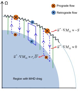
Figure 10: Sketch of mean meridional circulation and zonal flow off the equator in giant planet atmospheres. Straight blue lines with arrows indicate the mass circulation; green lines indicate $M_{\Omega}$ contours; wavy lines indicate eddy angular momentum fluxes. The size of the zonal-flow symbols is to suggest the speed of the flow. The blue shaded region represents the electrically conducting part of the atmosphere, where MHD drag acts.

The mean meridional circulation cells link the dynamics in the upper troposphere to the flow at depth, adjusting the thermal structure of the atmosphere between the upper troposphere and the layer where the drag acts such that the zonal-flow shear along $M_{\Omega}$ surfaces implied by thermal-wind balance becomes consistent with the balance (12) between eddy angular momentum flux divergences and drag. This is analogous to the role mean meridional circulations play in Earth’s atmosphere (e.g., Holton 2004, chapter 10).

Where the Rossby number is not small, the advection of angular momentum by the mean mass flux—the second term on the left-hand side of (5)—cannot be neglected and also contributes to the angular momentum balance and its density-weighted integral along $M_{\Omega}$ surfaces, as discussed in SL09. However, in the tropospheres of the giant planets, this appears to be significant only within a few degrees latitude of the equator (see SL09 and footnote 5).

c Implications for thermal structure

Jupiter, Saturn, and Neptune have sufficiently strong intrinsic heat fluxes to lead to convection in their tropospheres (Guillot et al. 2004; Guillot 2005), as in our simulations. The occurrence of convection and the expected homogenization of entropy along convective plumes further constrains the thermal structure of the tropospheres and thus, through thermal wind balance, the zonal flow structures.

In the giant planet tropospheres, the convective Rossby number is generally small, and viscous momentum dissipation and thermal diffusion are thought to be negligible. Under these circumstances, convective plumes are columns aligned with $M_{\Omega}$ surfaces, because, as above, rapid rotation inhibits motion perpendicular to $M_{\Omega}$ surfaces in the absence of viscous or other stresses (e.g., Busse 1976, 1978; Kaspi et al. 2009; Jones et al. 2009). Therefore, convection tends to homogenize entropy along columns in the direction of the planet’s spin axis (in deep atmospheres) or in the vertical (in thin atmospheres); however, it does not constrain entropy gradients in perpendicular directions. The forced-dissipative statistically steady state that results in the presence of vigorous convection thus is neutral with respect to slantwise convective instabilities, that is, convective and inertial axisymmetric instabilities (Emanuel 1983; Thorpe and Rotunno 1989; Emanuel 1994, chapter 12; Schneider 2007).

In our Jupiter, Saturn, and Neptune simulations, such a state with nearly convectively neutral interior tropospheres is indeed attained outside a few degrees of the equator (Fig. 5). The entropy and its meridional gradient hence do not vary in the vertical (e.g., Fig. 6), and neither does, by thermal wind balance, the shear (with respect to pressure) of the zonal flow. A corresponding state with entropy and its meridional gradient homogeneous in the direction of the spin axis can be expected to be attained on the actual planets, and thermal wind balance for deep atmospheres then similarly constrains the zonal flow. For a deep atmosphere in the anelastic approximation (valid for small fluctuations relative to an isentropic reference state), thermal wind balance reads

$$2\Omega\frac{\partial u}{\partial z}=-\frac{\alpha_{s}g}{r}\,\frac{\partial s}{\partial\phi},$$ (13)

where $z$ is the cylindrical height coordinate in the direction of the spin axis, $s$ is the specific entropy, and $\alpha_{s}(\rho)$ is a thermal expansion coefficient that relates entropy fluctuations to density fluctuations (Kaspi et al. 2009). That is, if the meridional entropy gradient does not vary in the direction of the spin axis, the shear of the zonal flow in the direction of the spin axis depends only on $\alpha_{s}$, $g$, and $r$, all of which generally vary ($\alpha_{s}$ and $g$ vary primarily with $r$). In Jupiter’s and Saturn’s upper tropospheres, the meridional entropy gradient and thus the zonal thermal wind shear approximately vanish at the zeros of the zonal wind (Simon-Miller et al. 2006; Read et al. 2006, 2009), as they do in our simulations (Fig. 5). To the extent that entropy deeper in the troposphere is homogenized in the direction of the spin axis, the thermal wind balance (13) suggests that the zonal flow shear then vanishes at all depths extending downward in the direction of the spin axis from the upper-tropospheric zeros of the zonal flow. So zeros of the zonal flow project downward along cylinders concentric with the spin axis.

In the literature on the giant planets, it is often taken as axiomatic that their interior tropospheres are rendered isentropic by convection, resulting in zonal flows (Taylor columns) without shear in the direction of the spin axis (e.g., Vasavada and Showman 2005). However, convection in general does not homogenize entropy in directions perpendicular to angular momentum surfaces, so an isentropic interior cannot be assumed a priori. The flow on the giant planets, where the Rossby number is small, must satisfy the constraints (8)–(12) dictated by the angular momentum balance, as well as thermal wind balance (13). Given that significant eddy angular momentum flux divergences in the upper tropospheres have been observed at least on Jupiter and Saturn, it is very unlikely that the zonal drag, which depends on the zonal flow, can balance the net eddy angular momentum flux divergence on an $M_{\Omega}$ surface without any shear of the zonal flow in the direction of the spin axis. It hence is very unlikely that the interiors of the giant planets are isentropic.

d Implications for role of drag

Significant eddy angular momentum flux divergences have been observed in Jupiter’s and Saturn’s upper tropospheres, but no mechanism has been proposed of how they could be balanced by opposing eddy angular momentum flux divergences at depth such the angular momentum balance (12) integrated over $M_{\Omega}$ surfaces is satisfied without a drag mechanism. On the other hand, coupling of the flow at depths at which the atmosphere is electrically conducting to the magnetic field is a plausible mechanism that generates MHD drag (Liu et al. 2008; see also the appendix). This MHD drag can close the angular momentum balance integrated over $M_{\Omega}$ surfaces. Therefore, we adopted as our working hypothesis that the MHD drag acting at depth couples to the flow in the upper atmosphere, although details such as how the MHD drag depends on the zonal flow are poorly understood. This approach gave statistically steady states in which the angular momentum balance is closed in a manner that is physically plausible and consistent with observations.

Outside a few degrees latitude of the equator, the upper-tropospheric dynamics are linked to the flow and any drag at depth along cylindrical $M_{\Omega}$ surfaces. Therefore, outside the tangent cylinder that just grazes the region of substantial MHD drag in the equatorial plane, the upper-tropospheric flow cannot be linked to drag at depth. We chose to represent this equatorial region of no effective drag on the upper-tropospheric flow in our thin-shell simulations by having an equatorial no-drag region. A no-drag region extending to $33^{\circ}$ latitude corresponds to assuming that the region of substantial MHD drag is confined within about $\cos(33^{\circ})=0.84$ planetary radii. It is doubtful that this is an accurate estimate for all giant planets (Liu et al. 2008). However, as we have shown in section 4d, where exactly the MHD drag acts, and how strong it is, does not affect the essence of our results.

The preceding discussion shows that simulations of only thin atmospheric shells can have closed energy and angular momentum balances that are physically plausible and consistent with observations of the giant planets. A model domain of sufficient depth to take into account the absorption of solar radiation in the upper atmosphere is essential to obtain baroclinic flows with an energy balance that is consistent with observations. Resolving baroclinic eddy fluxes of angular momentum in the upper atmosphere is essential to obtain an angular momentum balance that is consistent with observations. Drag at depth closes the balances in a physically plausible manner (e.g., without assuming excessive viscous stresses in the planetary interior). However, the depth of the nearly inviscid interior layer in which there are no significant heat sources and where $\mathcal{D}\approx 0$ and $\mathcal{S}\approx 0$ is immaterial for the mechanisms we discussed. The depth of that layer can be expected to affect quantitative aspects such as the vertical shear of the zonal flow, but we do not expect it to affect the qualitative aspects and large-scale flow features on which we have focused.

6 Conclusions

We have presented the first simulations of all four giant planets with closed energy and angular momentum balances that are consistent with observations. The simulations reproduce many large-scale features of the observed flows, such as equatorial superrotation on Jupiter and Saturn and equatorial subrotation on Uranus and Neptune. They exhibit temperature structures that are broadly consistent with available observations, and they reproduce many details of the observed flows, for example, their vertical structure to the extent it is known and characteristic equatorial waves observed on Jupiter. We have demonstrated that equatorial superrotation is generated if convective Rossby wave generation is strong and low-latitude angular momentum flux divergence owing to baroclinic eddies generated off the equator is sufficiently weak (Jupiter and Saturn); equatorial subrotation results if either convective Rossby wave generation is weak or absent (Uranus) or low-latitude angular momentum flux divergence owing to baroclinic eddies is sufficiently strong (Neptune).

Current computational resources limit our ability to simulate flows at depth. However, considerations of the angular momentum balance have shown that the zonal jets should extend—generally with shear—to the depth where drag acts on them and balances the angular momentum flux divergences and convergences in the upper troposphere. That drag acts on the zonal flow at depth is suggested by observations of eddy angular momentum fluxes on Jupiter and Saturn, and a plausible MHD drag mechanism exists. Though quantitative aspects (e.g., jet strength and shear) may be affected by our inability to resolve the flow and drag at depth, the jet formation mechanisms we discussed are not affected by it.

We expect as-yet unobserved aspects of the flow and temperature structures to be consistent with the simulations and mechanisms we presented. For example, we predict that NASA’s upcoming JUNO mission to Jupiter will find evidence of zonal flows with vertical shear similar to those in Fig. 5: near the equator, a strong and deep prograde jet, and away from the equator, prograde jets that weaken and retrograde jets that weaken only slightly or strengthen with depth. The thermal and gravitational signature of such zonal flows will likely be measurable by JUNO.

Acknowledgments

This work was supported by a David and Lucile Packard Fellowship. The GCM is based on the Flexible Modeling System of the Geophysical Fluid Dynamics Laboratory; the simulations were performed on Caltech’s Division of Geological and Planetary Sciences Dell cluster. We thank Andy Ingersoll and Yohai Kaspi for helpful discussions and comments on drafts of this paper.

APPENDIX A

General Circulation Model

a Resolution

The GCM solves the hydrostatic primitive equations using the spectral transform method in the horizontal and finite differences in the vertical. The horizontal spectral resolution depends on the radius of the planet being simulated (Table 1). The vertical coordinate is $\sigma=p/p_{s}$ (pressure $p$ normalized by pressure at lower boundary $p_{s}$); it is discretized with 30 levels for Jupiter and Saturn and 40 levels for Uranus and Neptune.

b Drag at lower boundary

All parameter choices are constrained by knowledge of the physical properties of the planets and material properties of their atmospheres, as well as by observations where available. However, the drag formulation at the artificial lower boundary of the GCM is poorly constrained by data or physics. It represents the MHD drag the flow experiences in the interior of the planets.

In the interior of Jupiter and Saturn, the conductivity of molecular hydrogen increases with depth and becomes approximately constant where hydrogen becomes metallic at $\mathop{\sim}\!1.4\,\mathrm{Mbar}$ (Nellis et al. 1996). In the interior of Uranus and Neptune, the conductivity of the gas envelope likewise increases with depth and is determined by the conductivity of hydrogen and water ice (Nellis et al. 1997). In the high-conductivity interior, the interaction of the magnetic field and the fluid flow produces Ohmic dissipation and retards the flow (Liu et al. 2008).

We represented this MHD drag deep in the atmosphere in the simplest possible way in our thin-shell GCM, choosing the same drag formulation and depth of the artificial lower boundary in all giant planet simulations, to rule out that differences among them are caused by differences in poorly constrained parameters. We assume linear (Rayleigh) drag acts near the GCM’s lower boundary, but only outside an equatorial latitude band (see SL09 and section 5d). As in the models in SL09 or Held and Suarez (1994), the drag coefficient decreases linearly from its value $k_{0}$ at the lower boundary at $\sigma=1.0$ to zero above $\sigma=0.8$. The equatorial no-drag region extends to $\phi_{0}=33^{\circ}$ latitude in all our simulations, corresponding to a MHD drag that acts only within $0.84$ planetary radii. The drag coefficient is constant ($k_{0}=10^{-2}\,\mathrm{days^{-1}}$) outside this region. The kinetic energy dissipated by the Rayleigh drag (a few percent of the sum of the intrinsic heat flux and the absorbed solar radiative flux) is returned to the flow locally as heat to conserve energy.

We chose the width of the no-drag region and the drag coefficient outside of it empirically, to obtain jets in the upper atmosphere that have similar strength and width as the observed jets. By choosing drag formulations that differ from planet to planet, better fits to observations could be obtained (cf. section 4d).

c Radiative transfer

As in SL09, radiative transfer is represented as that in a homogeneous gray atmosphere, using the two-stream approximation. The top-of-atmosphere (TOA) insolation is imposed as perpetual equinox with no diurnal cycle, $F_{\mathrm{TOA}}=(F_{0}/\pi)\cos\phi$, with the appropriate solar constant $F_{0}$ for each planet (Table 1). That is, for the purposes of this paper, we ignore the seasonal cycle in TOA insolation, which is substantial for Saturn, Uranus, and Neptune because of their obliquities. Ignoring seasonality may be justifiable, for example, if response timescales of the atmospheric circulation (e.g., radiative timescales) are much longer than seasonal timescales, which may be the case on the giant planets. However, the nonzero obliquities also influence the annual-mean TOA insolation, especially on Uranus, an influence we likewise ignore.

The solar radiative flux for a semi-infinite scattering and absorbing atmosphere is calculated for a solar optical depth $\tau_{s}$ that is linear in pressure, $\tau_{s}=\tau_{s0}(p/p_{0})$, to represent scattering and absorption by a well-mixed absorber. The solar optical properties of the giant planet atmospheres are not well constrained. To minimize differences among the simulations, we chose the same solar optical properties for all giant planets: $\tau_{s0}=3.0$ at $p_{0}=3.0$ bar. This gives a solar radiative flux qualitatively consistent with Galileo probe measurements in Jupiter (Sromovsky et al. 1998).

The thermal radiative flux is calculated for a gray atmosphere in which the thermal optical depth $\tau_{l}$ is quadratic in pressure, $\tau_{l}=\tau_{l0}(p/p_{0})^{2}$, to represent collision-induced absorption of thermal radiation. The thermal optical depths $\tau_{l0}$ at pressure $p_{0}$ are chosen such that the observed thermal emission levels (e.g., Ingersoll 1990) of the giant planets approximately correspond to $\tau_{l}=1$. The thermal optical depths thus vary from planet to planet (Table 1).

The lower boundary condition for the radiative fluxes is energy conservation: the upward thermal radiative flux is set equal to the sum of the downward solar flux and thermal radiative flux at each grid point.

d Intrinsic heat flux

A spatially uniform and temporally constant heat flux, corresponding to that estimated for the giant planets (Table 1), is deposited in the GCM’s lowest layer to mimic intrinsic heat fluxes.

e Convection scheme

A quasi-equilibrium convection scheme represents (dry) convection. It relaxes temperature profiles toward a convective profile with adiabatic lapse rate $\Gamma=g/c_{p}$ (Schneider and Walker 2006). The convective relaxation time is chosen to be roughly the time it takes a gravity wave with speed $c$ to traverse the extratropical Rossby radius $L_{x}=c/f$, that is, roughly an extratropical inertial time $f^{-1}$. We chose the convective relaxation time to be $6\,\mathrm{hr}$ for Jupiter and Saturn and $10\,\mathrm{hr}$ for Uranus and Neptune. We experimented with convective relaxation times up to a factor 2 smaller and a factor 4 larger in preliminary simulations; the simulated flows appeared not to be sensitive to such variations of the relaxation time.

The convection scheme does not transport momentum, that is, it assumes a convective Prandtl number of zero. Prandtl numbers for dry convection are usually greater than zero, so this represents an idealization, which may affect our results. However, the convective generation of Rossby waves on which we focus occurs in the equatorial upper troposphere, where the vertical shear is relatively small (Fig. 5). So one may expect convective momentum fluxes not to alter our results substantially. But to the extent that the vertical shear and convective momentum fluxes cannot be neglected, they may amplify the superrotation in the upper troposphere in the Jupiter and Saturn simulations, as the equatorial zonal flow in those simulations is stronger at depth than in the upper troposphere, so that convection can be expected to transport momentum upward. The dependence of our results on the convective Prandtl number is worth investigating further.

f Subgrid-scale dissipation

For $\sigma\leq 0.8$, above the layer with Rayleigh drag, horizontal hyperdiffusion in the vorticity, divergence, and temperature equations is the only frictional process. The hyperdiffusion is represented by an exponential cutoff filter (Smith et al. 2002), with a damping time scale of 2 h at the smallest resolved scale. The cutoff wavenumber depends on the horizontal resolution (Table 1).

The energy dissipated by the subgrid-scale hyperdiffusion is not returned to the flow as heat. However, it amounts to less than $1\%$ of the total energy uptake of the atmosphere in all simulations.

g Simulations

The simulations were spun-up from an isothermal rest state, with small perturbations in temperature and vorticity to break the axisymmetry of the initial state. Each simulation was integrated for at least 40,000 Earth days. In the statistically steady states, the global-mean outgoing thermal radiative flux is within $1\%$ of the sum of the global-mean solar radiative flux and the imposed intrinsic heat flux. The vertically integrated Rayleigh drag on the zonal flow approximately balances the vertically integrated total (mean plus eddy) angular momentum flux convergence. The circulation statistics shown are computed from flow fields sampled 4 times daily and averaged over 1500 days. They were first computed on the GCM’s sigma surfaces, with the appropriate surface pressure-weighting of the averages (Schneider and Walker 2006), and then interpolated to pressure surfaces for display purposes.

References

- Allison et al. (1990) Allison, M., D. A. Godfrey, and R. F. Beebe, 1990: A wave dynamical interpretation of Saturn’s polar hexagon. Science, 247, 1061–1063.
- Andrews and McIntyre (1976) Andrews, D. G., and M. E. McIntyre, 1976: Planetary waves in horizontal and vertical shear: The generalized Eliassen-Palm relation and the mean zonal acceleration. J. Atmos. Sci., 33, 2031–2048.
- Andrews and McIntyre (1978) , and , 1978: An exact theory of nonlinear waves on a Lagrangian-mean flow. J. Fluid Mech., 89, 609–646.
- Atkinson et al. (1998) Atkinson, D. H., J. B. Pollack, and A. Seiff, 1998: The Galileo probe Doppler wind experiment: Measurement of the deep zonal winds on Jupiter. J. Geophys. Res., 103, 22 911–22 928.
- Atreya et al. (1999) Atreya, S. K., M. H. Wong, T. C. Owen, P. R. Mahaffy, H. B. Niemann, I. de Pater, P. Drossart, and T. Encrenaz, 1999: A comparison of the atmospheres of Jupiter and Saturn: Deep atmospheric composition, cloud structure, vertical mixing, and origin. Planet. Space Sci., 47, 1243–1262.
- Aurnou et al. (2007) Aurnou, J., M. Heimpel, and J. Wicht, 2007: The effects of vigorous mixing in a convective model of zonal flow on the ice giants. Icarus, 190, 110–126.
- Busse (1976) Busse, F. H., 1976: A simple model of convection in the Jovian atmosphere. Icarus, 29, 255–260.
- Busse (1978) , 1978: Non-linear properties of thermal convection. Rep. Prog. Phys., 41, 1930–1967.
- Chan and Mayr (2008) Chan, K. L., and H. G. Mayr, 2008: A shallow convective model for Jupiter’s alternating wind bands. J. Geophys. Res., 113, E10 002. Doi:10.1029/2008JE003124.
- Charney (1963) Charney, J. G., 1963: A note on large-scale motions in the tropics. J. Atmos. Sci., 20, 607–609.
- Charney and Drazin (1961) , and P. G. Drazin, 1961: Propagation of planetary-scale disturbances from the lower into the upper atmosphere. J. Geophys. Res., 66, 83–109.
- Danilov and Gurarie (2002) Danilov, S., and D. Gurarie, 2002: Rhines scale and spectra of the -plane turbulence with bottom drag. Phys. Rev. E, 65. Art. no. 067301.
- Del Genio et al. (2007) Del Genio, A. D., J. M. Barbara, J. Ferrier, A. P. Ingersoll, R. A. West, A. R. Vasavada, J. Spitale, and C. C. Porco, 2007: Saturn eddy momentum fluxes and convection: First estimates from Cassini images. Icarus, 189, 479–492.
- Dritschel and McIntyre (2008) Dritschel, D. G., and M. E. McIntyre, 2008: Multiple jets as PV staircases: The Phillips effect and the resilience of eddy-transport barriers. J. Atmos. Sci., 65, 855–874.
- Emanuel (1983) Emanuel, K. A., 1983: On assessing local conditional symmetric instability from atmospheric soundings. Mon . Wea. Rev., 111, 2016–2033.
- Emanuel (1994) , 1994: Atmospheric Convection. Oxford University Press, 580 pp.
- Fletcher et al. (2007) Fletcher, L. N., and Coauthors, 2007: Characterising Saturn’s vertical temperature structure from CassiniCIRS. Icarus, 189, 457–478.
- Fletcher et al. (2008) , and Coauthors, 2008: Temperature and composition of Saturn’s polar hot spots and hexagon. Science, 319, 79–81.
- Gibbard et al. (2003) Gibbard, S. G., I. de Pater, H. G. Roe, S. Martin, B. A. Macintosh, and C. E. Max, 2003: The altitude of Neptune cloud features from high-spatial-resolution near-infrared spectra. Icarus, 166, 359–374.
- Gierasch et al. (2000) Gierasch, P. J., and Coauthors, 2000: Observation of moist convection in Jupiter’s atmosphere. Nature, 403, 628–630.
- Gill (1982) Gill, A. E., 1982: Atmosphere-Ocean Dynamics. International Geophysics Series, Vol. 30, Academic Press, 662 pp.
- Godfrey (1988) Godfrey, D. A., 1988: A hexagon feature around Saturn’s north pole. Icarus, 76, 335–356.
- Guillot (1999) Guillot, T., 1999: A comparison of the interiors of Jupiter and Saturn. Plan. Space Sci., 47, 1183–1200.
- Guillot (2005) , 2005: The interiors of giant planets: Models and outstanding questions. Ann. Rev. Earth Planet. Sci., 33, 493–530.
- Guillot et al. (2004) , D. J. Stevenson, W. B. Hubbard, and D. Saumon, 2004: The interior of Jupiter. F. Bagenal, T. E. Dowling, and W. B. McKinnon, Eds., Jupiter: The Planet, Satellites and Magnetosphere, Cambridge University Press, 35–57.
- Hammel et al. (2001) Hammel, H. B., K. Rages, G. W. Lockwood, E. Karkoschka, and I. de Pater, 2001: New measurements of the winds of Uranus. Icarus, 153, 229–235.
- Hammel et al. (2005) , I. de Pater, S. Gibbard, G. W. Lockwood, and K. Rages, 2005: Uranus in 2003: Zonal winds, banded structure, and discrete features. Icarus, 175, 534–545.
- Hanel et al. (1981) Hanel, R. A., B. J. Conrath, L. W. Herath, V. G. Kunde, and J. A. Pirraglia, 1981: Albedo, internal heat, and energy balance of Jupiter—Preliminary results of the Voyager infrared investigation. J. Geophys. Res, 86, 8705–8712.
- Hanel et al. (1983) , , V. G. Kunde, J. C. Pearl, and J. A. Pirraglia, 1983: Albedo, internal heat flux, and energy balance of Saturn. Icarus, 53, 262–285.
- Haynes et al. (1991) Haynes, P. H., C. J. Marks, M. E. McIntyre, T. G. Shepherd, and K. P. Shine, 1991: On the downward control of extratropical diabatic circulations by eddy-induced mean zonal forces. J. Atmos. Sci., 48, 651–679.
- Heimpel and Aurnou (2007) Heimpel, M., and J. Aurnou, 2007: Turbulent convection in rapidly rotating spherical shells: A model for equatorial and high latitude jets on Jupiter and Saturn. Icarus, 187, 540–557.
- Heimpel et al. (2005) , , and J. Wicht, 2005: Simulation of equatorial and high-latitude jets on Jupiter in a deep convection model. Nature, 438, 193–196.
- Held (1975) Held, I. M., 1975: Momentum transport by quasi-geostrophic eddies. J. Atmos. Sci., 32, 1494–1497.
- Held (2000) , 2000: The general circulation of the atmosphere. Proc. Program in Geophysical Fluid Dynamics, Woods Hole Oceanographic Institution, Woods Hole, MA. URL https://darchive.mblwhoilibrary.org/handle/1912/15.
- Held and Suarez (1994) Held, I. M., and M. J. Suarez, 1994: A proposal for the intercomparison of the dynamical cores of atmospheric general circulation models. Bull. Amer. Meteor. Soc., 75, 1825–1830.
- Holton (2004) Holton, J. R., 2004: An Introduction to Dynamic Meteorology. International Geophysics Series, Vol. 88, 4th ed., Elsevier, 547 pp.
- Hubbard et al. (1991) Hubbard, W. B., W. J. Nellis, A. C. Mitchell, N. C. Holmes, S. S. Limaye, and P. C. McCandless, 1991: Interior structure of Neptune: Comparison with Uranus. Science, 253, 648–651.
- Ingersoll (1976) Ingersoll, A. P., 1976: Pioneer 10 and 11 observations and the dynamics of Jupiter’s atmosphere. Icarus, 29, 245–253.
- Ingersoll (1990) , 1990: Atmosphere dynamics of the outer planets. Science, 248, 308–315.
- Ingersoll and Porco (1978) , and C. C. Porco, 1978: Solar heating and internal heat flow on Jupiter. Icarus, 35, 27–43.
- Ingersoll et al. (1981) , R. F. Beebe, J. L. Mitchell, G. W. Garneau, G. M. Yagi, and J.-P. Müller, 1981: Interaction of eddies and mean zonal flow on Jupiter as inferred from Voyager 1 and 2 images. J. Geophys. Res., 86, 8733–8743.
- Ingersoll et al. (1976) , G. Münch, G. Neugebauer, and G. S. Orton, 1976: Results of the infrared radiometer experiment on Pioneers 10 and 11. T. Gehrels, Ed., Jupiter: Studies of the interior, atmosphere, magnetosphere and satellites, University of Arizona Press, 197–205.
- Ingersoll et al. (2000) , P. J. Gierasch, D. Banfield, A. R. Vasavada, and the Galileo Imaging Team, 2000: Moist convection as an energy source for the large-scale motions in Jupiter’s atmosphere. Nature, 403, 630–632.
- Ingersoll et al. (2004) , and Coauthors, 2004: Dynamics of Jupiter’s atmosphere. F. Bagenal, T. E. Dowling, and W. B. McKinnon, Eds., Jupiter: The Planet, Satellites and Magnetosphere, Cambridge University Press, 105–128.
- Jones et al. (2009) Jones, C. A., K. M. Kuzanyan, and R. H. Mitchell, 2009: Linear theory of compressible convection in rapidly rotating spherical shells, using the anelastic approximation. J. Fluid Mech., 634, 291–319.
- Kaspi et al. (2009) Kaspi, Y., G. R. Flierl, and A. P. Showman, 2009: The deep wind structure of the giant planets: results from an anelastic general circulation model. Icarus, 202, 525–542.
- Levine et al. (1977) Levine, J. S., D. R. Kraemer, and W. R. Kuhn, 1977: Solar radiation incident on Mars and the outer planets: Latitudinal, seasonal, and atmospheric effects. Icarus, 31, 136–145.
- Lian and Showman (2008) Lian, Y., and A. P. Showman, 2008: Deep jets on gas-giant planets. Icarus, 194, 597–615.
- Lian and Showman (2010) , and , 2009: Generation of equatorial jets by large-scale latent heating on giant planets. Icarus, 207, 373–393.
- Liu et al. (2008) Liu, J. J., P. M. Goldreich, and D. J. Stevenson, 2008: Constraints on deep-seated zonal winds inside Jupiter and Saturn. Icarus, 196, 653–664.
- Lodders and B. Fegley (1998) Lodders, K., and J. B. Fegley, 1998: The Planetary Scientist’s Companion. Oxford University Press, 400 pp.
- Lorenz (1955) Lorenz, E. N., 1955: Available potential energy and the maintenance of the general circulation. Tellus, 7, 157–167.
- Marcus (1988) Marcus, P. S., 1988: Numerical simulation of Jupiter’s Great Red Spot. Nature, 331, 693–696.
- Marcus (1993) , 1993: Jupiter’s Great Red Spot and other vortices. Annu. Rev. Astron. Astronphys., 31, 523–573.
- Matsuno (1966) Matsuno, T., 1966: Quasi-geostrophic motions in the equatorial area. J. Meteor. Soc. Japan, 44, 25–42.
- McIntyre (1982) McIntyre, M. E., 1982: How well do we understand the dynamics of stratospheric warmings? J. Meteor. Soc. Japan, 60, 37–65.
- McWilliams (1984) McWilliams, J. C., 1984: The emergence of isolated coherent vortices in turbulent flow. J. Fluid Mech., 146, 21–43.
- Nellis et al. (1996) Nellis, W. J., S. T. Weir, and A. C. Mitchell, 1996: Metallization and electrical conductivity of hydrogen in Jupiter. Science, 273, 936–938.
- Nellis et al. (1997) , N. C. Holmes, A. C. Mitchell, D. C. Hamilton, and M. Nicol, 1997: Equation of state and electrical conductivity of “synthetic Uranus,” a mixture of water, ammonia, and isopropanol, at shock pressure up to 200 GPa (2 Mbar). J. Chem. Phys., 107, 9096–9100.
- O’Gorman and Schneider (2008) O’Gorman, P. A., and T. Schneider, 2008: Weather-layer dynamics of baroclinic eddies and multiple jets in an idealized general circulation model. J. Atmos. Sci., 65, 524–535.
- Peixoto and Oort (1992) Peixoto, J. P., and A. H. Oort, 1992: Physics of Climate. American Institute of Physics, 555 pp.
- Porco et al. (2003) Porco, C. C., and Coauthors, 2003: Cassini imaging of Jupiter’s atmosphere, satellites, and rings. Science, 299, 1541–1547.
- Read et al. (2006) Read, P. L., P. J. Gierasch, B. J. Conrath, A. Simon-Miller, T. Fouchet, and Y. H. Yamazaki, 2006: Mapping potential-vorticity dynamics on Jupiter. I. Zonal-mean circulation from Cassini and Voyager 1 data. Quart. J. Roy. Meteor. Soc., 132, 1577–1603.
- Read et al. (2009) , B. J. Conrath, L. N. Fletcher, P. J. Gierasch, A. A. Simon-Miller, and L. C. Zuchowski, 2009: Mapping potential vorticity dynamics on Saturn: Zonal mean circulation from Cassini and Voyager data. Planet. Space Sci., 57, 1682–1698.
- Rhines (1994) Rhines, P. B., 1994: Jets. Chaos, 4, 313–339.
- Salyk et al. (2006) Salyk, C., A. P. Ingersoll, J. Lorre, A. Vasavada, and A. D. Del Genio, 2006: Interaction between eddies and mean flow in Jupiter’s atmosphere: Analysis of Cassini imaging data. Icarus, 185, 430–442.
- Sanchez-Lavega et al. (2003) Sanchez-Lavega, A., S. Perez-Hoyos, J. F. Rojas, R. Hueso, and R. G. French, 2003: A strong decrease in Saturn’s equatorial jet at cloud level. Nature, 423, 623–625.
- Sanchez-Lavega et al. (2007) , R. Hueso, and S. Perez-Hoyos, 2007: The three-dimensional structure of Saturn’s equatorial jet at cloud level. Icarus, 187, 510–519.
- Sardeshmukh and Hoskins (1988) Sardeshmukh, P. D., and B. J. Hoskins, 1988: The generation of global rotational flow by steady idealized tropical divergence. J. Atmos. Sci., 45, 1228–1251.
- Schneider (2007) Schneider, T., 2007: The thermal stratification of the extratropical troposphere. T. Schneider and A. H. Sobel, Eds., The Global Circulation of the Atmosphere, Princeton University Press, 47–77.
- Schneider and Walker (2006) , and C. C. Walker, 2006: Self-organization of atmospheric macroturbulence into critical states of weak nonlinear eddy-eddy interactions. J. Atmos. Sci., 63, 1569–1586.
- Schneider and Liu (2009) , and J. Liu, 2009: Formation of jets and equatorial superrotation on Jupiter. J. Atmos. Sci., 66, 579–601.
- Scott and Polvani (2008) Scott, R. K., and L. M. Polvani, 2008: Equatorial superrotation in shallow atmospheres. Geophys. Res. Lett., 35, L24 202.
- Simon-Miller et al. (2006) Simon-Miller, A. A., B. J. Conrath, P. J. Gierasch, G. S. Orton, R. K. Achterberg, F. M. Flasar, and B. M. Fisher, 2006: Jupiter’s atmospheric temperatures: From Voyager IRIS to Cassini CIRS. Icarus, 180, 98–112.
- Smith et al. (2002) Smith, K. S., G. Boccaletti, C. C. Henning, I. Marinov, C. Y. Tam, I. M. Held, and G. K. Vallis, 2002: Turbulent diffusion in the geostrophic inverse cascade. J. Fluid. Mech., 469, 13–48.
- Sobel et al. (2001) Sobel, A. H., J. Nilsson, and L. M. Polvani, 2001: The weak temperature gradient approximation and balanced tropical moisture waves. J. Atmos. Sci., 58, 3650–3665.
- Sromovsky et al. (1998) Sromovsky, L. A., A. D. Collard, P. M. Fry, G. S. Orton, M. T. Lemmon, M. G. Tomasko, and R. S. Freedman, 1998: Galileo probe measurements of thermal and solar radiation fluxes in the Jovian atmosphere. J. Geophys. Res., 103, 22 929–22 977.
- Sromovsky et al. (2001) , P. M. Fry, T. E. Dowling, K. H. Baines, and S. S. Limaye, 2001: Coordinated 1996 HST and IRTF imaging of Neptune and Triton. III. Neptune’s atmospheric circulation and cloud structure. Icarus, 149, 459–488.
- Thorpe and Rotunno (1989) Thorpe, A. J., and R. Rotunno, 1989: Nonlinear aspects of symmetric instability. J. Atmos. Sci., 46, 1285–1299.
- Vallis (2006) Vallis, G. K., 2006: Atmospheric and Oceanic Fluid Dynamics: Fundamentals and Large-Scale Circulation. Cambridge University Press, 771 pp.
- Vasavada and Showman (2005) Vasavada, A. R., and A. P. Showman, 2005: Jovian atmospheric dynamics: an update after Galileo and Cassini. Rep. Prog. Phys., 68, 1935–1996.
- Williams (1979) Williams, G. P., 1979: Planetary circulations: 2. The Jovian quasi-geostrophic regime. J. Atmos. Sci., 36, 932–968.
- Williams (2003a) , 2003a: Barotropic instability and equatorial superrotation. J. Atmos. Sci., 60, 2136–2152.
- Williams (2003b) , 2003b: Jovian dynamics. Part III: Multiple, migrating, and equatorial jets. J. Atmos. Sci., 60, 1270–1296.
- Yamazaki et al. (2005) Yamazaki, Y., P. Read, and D. Skeet, 2005: Hadley circulations and Kelvin wave-driven equatorial jets in the atmospheres of Jupiter and Saturn. Planet. Space Sci., 53, 508–525.