Cosmic neutrinos at IceCube: $\theta_{13}$, $\delta$ and initial flavor composition

Abstract

We discuss the prospect of extracting the values of the mixing parameters $\delta$ and $\theta_{13}$ through the detection of cosmic neutrinos in the planned and forthcoming neutrino telescopes. We take the ratio of the $\mu$-track to shower-like events, $R$, as the realistic quantity that can be measured in the neutrino telescopes. We take into account several sources of uncertainties that enter the analysis. We then examine to what extent the deviation of the initial flavor composition from $w_{e}:w_{\mu}:w_{\tau}=1:2:0$ can be tested.

The neutrino mixing parameters can be extracted from cosmic neutrinos data according to the following argument [1]: assume that the flavor ratio of neutrinos at the source is $w_{e}:w_{\mu}:w_{\tau}$; after that neutrinos travel the large distances between the astrophysical sources and the Earth the oscillatory terms in the flavor transition probabilities average out such that the flavor ratio at the detector will become

$$\sum_{\alpha}w_{\alpha}P_{\alpha e}:\sum_{\alpha}w_{\alpha}P_{\alpha\mu}:\sum_{\alpha}w_{\alpha}P_{\alpha\tau},$$ (1)

where

$$P_{\alpha\beta}\equiv P(\nu_{\alpha}\to\nu_{\beta})=P(\bar{\nu}_{\alpha}\to\bar{\nu}_{\beta})=\sum_{i}|U_{\alpha i}|^{2}|U_{\beta i}|^{2},$$ (2)

and $U_{\alpha i}$ are the elements of the neutrino mixing matrix. In a wide range of models the flavor ratios at the source are predicted to be $w_{e}:w_{\mu}:w_{\tau}=1:2:0$. Thus, by measuring the flavor ratio at Earth, one can derive the absolute values of the mixing matrix elements which in principle yield information on the yet-unknown neutrino parameters $\theta_{13}$ and $\delta$.

IceCube [2] and its Mediterranean counterparts ( such as KM3NET [3]) can basically distinguish only two types of events: 1) shower-like events; 2) $\mu$-track events. It is possible to derive information on the flavor composition of neutrinos by studying the ratio $R=$number of $\mu$-track events/number of shower-like events [4]. In the analysis in this paper we consider neutrinos with energies 100 GeV $<E_{\nu}<$ 100 TeV, where the upper and lower limits come from the absorption of neutrinos in Earth and the energy threshold of detection in neutrino telescopes, respectively.

Two sources contribute to the $\mu$-track events: (i) Charged Current (CC) interaction of $\nu_{\mu}$ or $\bar{\nu}_{\mu}$ producing $\mu$ or $\bar{\mu}$; (ii) CC interaction of $\nu_{\tau}$ and $\bar{\nu}_{\tau}$ producing $\tau$ or $\bar{\tau}$ and the subsequent decay of $\tau$ and $\bar{\tau}$ into $\mu$ and $\bar{\mu}$. In the literature, the contribution of $\nu_{\tau}$ (via $\nu_{\tau}\to\tau\to\mu$) to $\mu$-track events has been overlooked but to study the effect of $\theta_{13}$, one should take into account such sub-dominant effects (see the Appendix of [5] for details). Three types of events appear as shower: i) the Neutral Current (NC) interactions of all kinds of neutrinos; ii) the CC interactions of $\nu_{e}$ and $\bar{\nu}_{e}$; iii) the CC interactions of $\nu_{\tau}$ ($\bar{\nu_{\tau}}$) and the subsequent hadronic decay of $\tau$ ($\bar{\tau}$). Details of the event rate calculation for each case in both $\mu$-track and shower-like events can be found in [5].

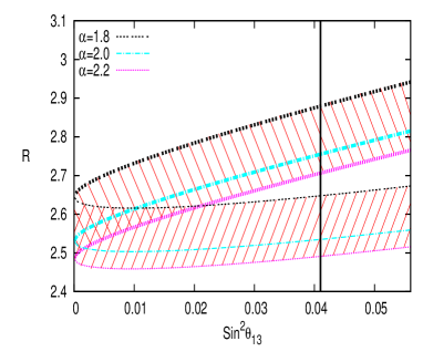
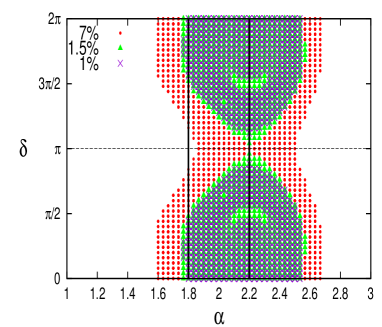
       (a)                                                                             (b)

Figure 1: (a) The dependence of $R$ on $\sin^{2}\theta_{13}$ for different values of the spectral index, $\alpha$. The thicker lines correspond to $\delta=\pi$ and the thinner ones correspond to $\delta=0$. In drawing this figure we have set $\mathcal{N}_{\bar{\nu}_{e}}/\mathcal{N}_{\nu_{e}}=0.5$ and $(\mathcal{N}_{\bar{\nu}_{\mu}}+\mathcal{N}_{\nu_{\mu}})/(\mathcal{N}_{\bar{\nu}_{e}}+\mathcal{N}_{\nu_{e}})=2$. The input for $\theta_{12}$ and $\theta_{23}$ are set equal to the best fit in [6]. The vertical line at 0.041 shows the present bound at 3$\sigma$ [6] (b) Points in the $(\alpha,\delta)$ space consistent with $R=2.53\pm\Delta R$. True values of the $(\alpha,\delta)$ pair are $(2,\pi/2)$. Points displayed by dots, triangles and crosses respectively correspond to $\Delta R/\bar{R}=7\%$, $\Delta R/\bar{R}=1.5\%$ and $\Delta R/\bar{R}=1\%$. To draw this figure we have varied $\sin^{2}\theta_{13}\in(0.028,0.032)$, $\sin^{2}\theta_{12}\in(0.30,0.34)$, $\sin^{2}\theta_{23}\in(0.47,0.53)$ and $\mathcal{N}_{\bar{\nu}_{e}}/\mathcal{N}_{{\nu}_{e}}\in(0,1)$.

Several input parameters enter the calculation of $R$ and their uncertainties induce imprecision in the calculated value of $R$. We consider the following uncertainties in the calculation of $R$: i) for the energy spectrum of neutrinos we assume a power-law spectrum $dF_{\nu_{\beta}}/dE_{\nu_{\beta}}=\mathcal{N}_{\nu_{\beta}}E^{-\alpha}_{\nu_{\beta}}$. Neutrino production through the Fermi acceleration mechanism of particles in the source predict the value of the spectral index equal to $\alpha=2$, but taking into account non-linear effects in the acceleration mechanism results in spectral index values $\alpha\in(1,3)$. It is shown in [4] by assuming the flux $E_{\nu}^{2}dF_{\nu}/dE_{\nu}=0.25$ GeV cm^-2 sr^-1 yr^-1, after one year of data-taking $\alpha$ can be determined with 10% uncertainty. For the normalization factor $\mathcal{N}_{\nu_{\beta}}$ it can be shown that: $\mathcal{N}_{\bar{\nu}_{\mu}}=\mathcal{N}_{\nu_{\mu}}$ and $\mathcal{N}_{\bar{\nu}_{e}}/\mathcal{N}_{\nu_{e}}\in(0,1)$.

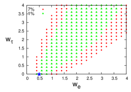
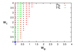
       (a)                                                           (b)

Figure 2: Points in the $(w_{e},w_{\tau})$ plane consistent with $R=\bar{R}\pm\Delta R$. The ratios are normalized such that $w_{\mu}=1$. The true values of $(w_{e},w_{\tau})$ are denoted by $\bigstar$. Points displayed by dots and triangles respectively correspond to $\Delta R/\bar{R}=7\%$ and $\Delta R/\bar{R}=1\%$. In drawing this figure we have varied $\sin^{2}\theta_{13}\in(0,0.003)$, $\delta\in(0,2\pi)$, $\alpha\in(1.8,2.2)$, and $\mathcal{N}_{\bar{\nu}_{e}}/\mathcal{N}_{{\nu}_{e}}\in(0,1)$. Drawing Fig. (a), we have taken $\bar{R}=2.53$ which corresponds to the standard picture with $w_{e}=1/2$ and $w_{\tau}=0$. In case Fig. (b), we have set $\bar{R}=3.2$ which corresponds to the stopped muon scenario with $w_{e}=w_{\tau}=0$.

Fig. (1-a) shows $R$ versus $\sin^{2}\theta_{13}$ for $\cos\delta=\pm 1$ and various values of $\alpha$. As seen from the figure when $\delta=0$, the sensitivity of $R$ to $s_{13}^{2}$ is very mild and less than 2 %. That is while for $\cos\delta=-1$, the sensitivity to $s_{13}^{2}$ is about 10 %. As seen from the figure, even for $\cos\delta=-1$, the sensitivity to $s_{13}^{2}$ can be obscured by the 10 % uncertainty in $\alpha$. However, for $s_{13}^{2}>0.02$, the bands between $\alpha=2.2$ and $1.8$ for $\cos\delta=1$ and $\cos\delta=-1$ have no overlap. This means that for $s_{13}^{2}>0.02$, 10 % precision in $\alpha$ is enough to distinguish $\cos\delta=1$ from $\cos\delta=-1$.

Fig. (1-b) addresses the question that whether it will be possible to extract the value of $\delta$. Drawing the plot, we have assumed that $\bar{R}$ will be found to have a typical value of 2.53 with an uncertainty of $\Delta R/\bar{R}$. This value of $\bar{R}$ can be obtained by taking maximal CP-violation $(\delta=\pi/2)$, $\sin^{2}\theta_{13}=0.03$, $w_{e}:w_{\mu}:w_{\tau}=1:2:0$, $\alpha=2$ and $\mathcal{N}_{\bar{\nu}_{e}}/\mathcal{N}_{{\nu}_{e}}=0.5\$. We have looked for solutions in the $\delta-\alpha$ plane for which $R=2.53(1\pm\Delta R/\bar{R})$, varying the rest of the relevant parameters in the ranges indicated in the caption of Fig. (1-b). The regions covered with dots, little triangles and crosses respectively correspond to 7%, 1.5% and 1% precision in the measurement of $R$. As seen from the figure, with $\Delta R/\bar{R}=7\%$, $\delta$ cannot be constrained. In fact, any point between the vertical lines can be a solution. The figure shows that reducing $\Delta R/\bar{R}$ to 1% (but keeping the rest of the uncertainties as before), some parts of the solutions can be excluded. In particular, the region around $\delta=\pi$ will not be a solution anymore. Notice that along with $\delta=\pi/2$, $\delta=0$ is also a solution. This means that despite maximal CP-violation, the CP-violation cannot still be established.

Taking into account the relevant uncertainties in the input parameters, we look for values of $w_{e}:w_{\mu}:w_{\tau}$ that are consistent with $R=\bar{R}\pm\Delta R$. To perform this analysis, we take $\theta_{13}=0$. In Fig. (2), we consider two possibilities: (i) the standard case with $w_{e}:w_{\mu}:w_{\tau}=0.5:1:0$ leading to $\bar{R}=2.53$ (see Fig. 2-a); (ii) the case of stopped muons with $w_{e}:w_{\mu}:w_{\tau}=0:1:0$ yielding $\bar{R}=3.20$ (see Fig. 2-b). From these figures we observe that with a precision of $\Delta R/\bar{R}=7\%$, these two scenarios can be easily discriminated. These two can also be discriminated from the scenario in which the neutrino production mechanism is $n\to pe\bar{\nu}_{e}$ (i.e., $w_{e}:w_{\mu}:w_{\tau}=1:0:0$). When we restrict the analysis to $w_{\tau}=0$ (i.e., the case without exotic neutrino properties) from these figures we observe that the measurement of $R$ stringently constrains $w_{e}:w_{\tau}$ which in turn sheds light on the production mechanism. However, once the assumption of $w_{\tau}$ is relaxed, a wide range of $w_{e}:w_{\mu}:w_{\tau}$ can be a solution. For example, the exotic case of $w_{e}:w_{\mu}:w_{\tau}=0:0:1$ leads to the same value of $\bar{R}$ as the stopped muon scenario.

I am grateful Y. Farzan for useful discussions and comments. I would like to thank “Bonyad-e Melli-e Nokhbegan” for partial financial support.

References

References

[1]
J. F. Beacom et al.
Phys. Rev. D 69 (2004) 017303
[arXiv:hep-ph/0309267];
\nonumY. Farzan and A. Y. Smirnov,
Phys. Rev. D 65 (2002) 113001
[arXiv:hep-ph/0201105].
[2]
J. Ahrens et al. [IceCube Collaboration],
Astropart. Phys. 20 (2004) 507
[arXiv:astro-ph/0305196].
[3]
U. F. Katz,
Nucl. Instrum. Meth. A 567 (2006) 457
[arXiv:astro-ph/0606068].
[4]
J. F. Beacom et al.
Phys. Rev. D 68 (2003) 093005
[Erratum-ibid. D 72 (2005) 019901]
[arXiv:hep-ph/0307025].
[5]
A. Esmaili and Y. Farzan,
Nucl. Phys. B 821 (2009) 197
[arXiv:0905.0259 [hep-ph]].
[6]
T. Schwetz,
Phys. Scripta T127 (2006) 1
[arXiv:hep-ph/0606060].