Measurement of the Pseudoscalar Decay Constant $f_{D_{s}}$ Using $D_{s}^{+}\to\tau^{+}\nu$, $\tau^{+}\to\rho^{+}\overline{\nu}$ Decays

Abstract

Analyzing 600 pb^-1 of $e^{+}e^{-}$ collisions at 4170 MeV center-of-mass energy with the CLEO-c detector, we measure the branching fraction ${\cal B}(D_{s}^{+}\to\tau^{+}\nu)=(5.52\pm 0.57\pm 0.21)$% using the $\tau^{+}\to\rho^{+}\overline{\nu}$ decay mode. Combining with other CLEO measurements of ${\cal B}(D_{s}^{+}\to\tau^{+}\nu)$ we determine the pseudoscalar decay constant $f_{D_{s}}=(259.7\pm 7.8\pm 3.4$) MeV consistent with the value obtained from our $D_{s}^{+}\to\mu^{+}\nu$ measurement of ($257.6\pm 10.3\pm 4.3$) MeV. Combining these measurements we find a value of $f_{D_{s}}=(259.0\pm 6.2\pm 3.0$) MeV, that differs from the most accurate prediction based on unquenched lattice gauge theory of ($241\pm 3)$ MeV by 2.4 standard deviations. We also present the first measurements of ${\cal B}(D_{s}^{+}\to K^{0}\pi^{+}\pi^{0})=(1.00\pm 0.18\pm 0.04)$%, and ${\cal B}(D_{s}^{+}\to\pi^{+}\pi^{0}\pi^{0})=(0.65\pm 0.13\pm 0.03)$%, and measure a new value for ${\cal B}(D_{s}^{+}\to\eta\rho^{+})=(8.9\pm 0.6\pm 0.5)$%.

I Introduction

The purely leptonic decay of the $D_{s}^{+}$ meson occurs in the Standard Model (SM) via the annihilation of the constituent charm quark with the constituent anti-strange quark into a virtual $W^{+}$ boson that subsequently materializes as a lepton-antineutrino pair. The SM decay rate is given by Formula1

$$\Gamma(D_{s}^{+}\to\ell^{+}\nu)={{G_{F}^{2}}\over 8\pi}f_{D_{s}}^{2}m_{\ell}^{2}M_{D_{s}^{+}}\left(1-{m_{\ell}^{2}\over M_{D_{s}^{+}}^{2}}\right)^{2}\left|V_{cs}\right|^{2}~{}~{}~{},$$ (1)

where $M_{D_{s}^{+}}$ is the $D_{s}^{+}$ mass, $m_{\ell}$ is the mass of the charged final state lepton, $G_{F}$ is the Fermi coupling constant, $|V_{cs}|$ is a Cabibbo-Kobayashi-Maskawa matrix element, and $f_{D_{s}}$ is the “decay constant,” a parameter related to the overlap of the heavy and light quark wave-functions at zero spatial separation.

Measurements of $D_{s}^{+}\to\mu^{+}\nu$ and $D_{s}^{+}\to\tau^{+}\nu$ have been made with increasing precision recently, and a disagreement has emerged between the theoretical value of $f_{D_{s}}$ computed by Follana et al. Lat:Foll , and the average of these measurements Rosner-Stone ; PDG . It has been pointed out by Akeroyd and Mahmoudi AkeroydM that physics beyond the SM could contribute differently to $\mu^{+}\nu$ and $\tau^{+}\nu$ final states, so increased precision on each of these is important.

We report here on a new measurement of ${\cal{B}}(D_{s}^{+}\to\tau^{+}\nu)$ using the $\tau^{+}\to\rho^{+}\overline{\nu}$ decay mode. Previously CLEO has reported on this rate using the $\tau^{+}\to\pi^{+}\overline{\nu}$ and $\tau^{+}\to e^{+}\nu\overline{\nu}$ modes.

II Experimental Method

II.1 Selection of $D_{s}$ Candidates

The CLEO-c detector CLEODR is equipped to measure the momenta and directions of charged particles, identify them using specific ionization ($dE/dx$) and Cherenkov light (RICH) RICH , detect photons and determine their directions and energies.

In this study we use 600 pb^-1 of data produced in $e^{+}e^{-}$ collisions using the Cornell Electron Storage Ring (CESR) and recorded near a center-of-mass energy ($E_{\rm CM}$) of 4.170 GeV. At this energy the $e^{+}e^{-}$ annihilation cross-section into $D_{s}^{-}D_{s}^{*+}$ + $D_{s}^{*-}D_{s}^{+}$ is approximately 1 nb poling .

In this analysis we fully reconstruct a sample of $D_{s}^{-}$ in nine “tag” modes and then find candidate $\rho^{+}\to\pi^{+}\pi^{0}$ decays in this sample. (Mention of any specific decay implies the use of its charge-conjugate as well.) The tag selection is identical to that used in our $D_{s}^{+}\to\mu^{+}\nu$ paper that can be consulted for details Dstomunu . Briefly, we select candidates using their invariant masses. We require that the candidate energies are consistent with those expected of a $D_{s}$ or $D_{s}^{*}$ in $D_{s}D_{s}^{*}$ events. The invariant mass distribution for all tag candidates is shown in Fig. 1(a). Then we detect an additional photon candidate from the $D_{s}^{*}$ decay, and construct

$${\rm MM}^{*2}=\left(E_{\rm CM}-E_{D_{s}}-E_{\gamma}\right)^{2}-\left({\bf p}_{\rm CM}-{\bf p}_{D_{s}}-{\bf p}_{\gamma}\right)^{2},$$ (2)

where $E_{\rm CM}$ (${\bf p}_{\rm CM}$) is the center-of-mass energy (momentum), $E_{D_{s}}$ (${\bf p}_{D_{s}}$) is the energy (momentum) of the fully reconstructed $D_{s}^{-}$ tag, and $E_{\gamma}$ (${\bf p}_{\gamma}$) is the energy (momentum) of the additional photon. In performing this calculation we use a kinematic fit that constrains the decay products of the $D_{s}^{-}$ to the known $D_{s}$ mass and conserves overall momentum and energy. All photon candidates in the event are tried, except for those that are decay products of the $D_{s}^{-}$ tag candidate. Regardless of whether or not the photon forms a $D_{s}^{*}$ with the tag, for real $D_{s}^{*}D_{s}$ events the missing mass-squared MM^∗2, recoiling against the photon and the $D_{s}^{-}$ tag should peak at the $D_{s}^{+}$ mass-squared.

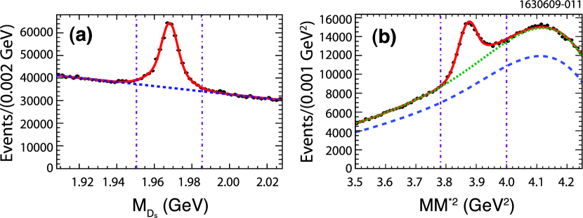
Figure 1: (a) Invariant mass of $D_{s}^{-}$ candidates summed over all decay modes and fit to a two-Gaussian signal shape plus a straight line for the background. The vertical dot-dashed lines indicate the $\pm$17.5 MeV definition of the signal region. No MM^∗2 cut has been applied. (b) The MM^∗2 distribution summed over all modes. The curves are fits to the number of signal events using the Crystal Ball function and two 5th order Chebyshev background functions; the dashed curve shows the background from fake $D_{s}^{-}$ tags, while the dotted curve in (b) shows the sum of the backgrounds from multiple photon combinations and fake $D_{s}^{-}$ tags. The vertical dashed lines show the region of events selected for further analysis.

The MM^∗2 distributions for events in the $D_{s}^{-}$ invariant mass signal region ($\pm$17.5 MeV from the $D_{s}$ mass) are shown in Fig. 1(b). In order to find the number of tags used for further analysis we perform a two-dimensional binned maximum liklihood fit of the MM^∗2 distribution and the invariant mass distribution in the interval $\pm$60 MeV from the $D_{s}$ mass and $3.50<{\rm MM}^{*2}<4.25$ GeV². The background has two components, both described by 5th order Chebyshev polynomials; the first comes from the background under the invariant mass peak, defined by the sidebands, and the second is due to multiple photon combinations. In both cases we allow the parameters to float.

We find a total of 43859$\pm$936$\pm$877 events within the interval $3.782<{\rm MM}^{*2}<4.000$ GeV² and having an invariant mass within $\pm$17.5 MeV of the $D_{s}$ mass, where the first uncertainty is statistical and the second is systematic.

II.2 Signal Reconstruction

We select events with one and only one charged track with opposite sign of charge to the tag, that is positively identified as a pion. The event also must contain at least one $\pi^{0}\to\gamma\gamma$ candidate with an invariant mass divided by the error on the invariant mass (Pull) $<$ 3; if there is more than one such candidate we choose the one with the minimum Pull. Tracks or photons that are used as part of the $D_{s}^{-}$ tag are not considered. Unfortunately, hadron tracks can and do interact in the detector material, and deposit additional energy in the electromagnetic calorimeter. Thus we do not reject events with more than one $\pi^{0}$ candidate. Photon candidates must have an energy deposition in the calorimeter consistent with that expected for an electromagnetic shower and deposit more than 30 MeV in the barrel or more than 50 MeV in the endcap. In principle for $D_{s}^{+}\to\tau^{+}\nu,~{}\tau^{+}\to\rho^{+}\overline{\nu}$ decays all the energy should be accounted for in the decay products of the tag and and the $\rho^{+}$. We sum up any energy in the calorimeter not matched with tag or the $\rho^{+}$ and call this parameter $E_{\rm extra}$.

We also compute the MM² as

$${\rm MM}^{2}=\left(E_{\rm CM}-E_{D_{s}}-E_{\gamma}-E_{\rho}\right)^{2}-\left({\bf p}_{\rm CM}-{\bf p}_{D_{s}}-{\bf p}_{\gamma}-{\bf p}_{\rho}\right)^{2},$$ (3)

where $E_{\rho}$ (${\bf p}_{\rho}$) are the energy (momentum) of the candidate $\rho^{+}$ and all other variables are the same as defined in Eq. (2). While the MM² does not peak at zero, because there are two missing neutrinos, it is still a useful variable as two-body $D_{s}^{+}$ decay backgrounds will peak; e.g., $D_{s}^{+}\to\rho^{+}\eta$ peaks at the $\eta$ mass-squared.

We proceed by defining a $\pi^{+}\pi^{0}$ mass window consistent with the $\rho^{+}$ mass. Fortunately, the mass distribution and the branching ratio for $\tau^{+}\to\rho^{+}\overline{\nu}$ decays are well measured Belle-tau-rhonu . We select events within $\pm$250 MeV of the $\rho^{+}$ mass. This selection is chosen to maximize efficiency while still not including too much background. This mass selection is 89.3% efficient for $\tau^{+}\to\rho^{+}\overline{\nu}$ events.

The expected MM² and $E_{\rm extra}$ distributions from signal Monte Carlo simulation of $D_{s}^{-}$ tag and $D_{s}^{+}\to\tau^{+}\nu$ events are shown in Fig. 2. Here we have included the above mentioned selection window on the $\pi^{+}\pi^{0}$ mass. The MM² signal shape is fit to a function that is the sum of two bifurcated-Gaussian functions. (A bifurcated-Gaussian shape has different widths below and above the mean.)

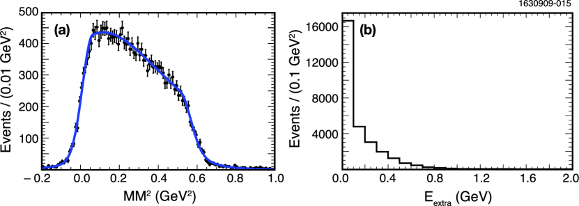
Figure 2: Monte Carlo generated distributions for signal $D_{s}^{+}\to\tau^{+}\nu$, $\tau^{+}\to\rho^{+}\overline{\nu}$ (a) MM², and (b) $E_{\rm extra}$. The curve in (a) is a fit to the data points with the sum of two bifurcated-Gaussian functions.

II.3 Background Expectations

There are two general sources of background expected arising from either combinatoric background in the reconstructed $D_{s}^{-}$ tag sample, or specific decay modes of the $D_{s}^{+}$. The former are determined by using sidebands of the candidate $D_{s}^{-}$ invariant mass distribution. The latter could arise from modes involving $\rho^{+}$ decays such as $\eta\rho^{+}$, but could also come from any mode that includes a $\pi^{+}$ and a $\pi^{0}$, or a $\pi^{+}$ and extra energy that is called a $\pi^{0}$. Previous studies have shown that requiring the $\pi^{+}$ candidate to project to the primary event vertex eliminates fake charged tracks as a background source oldDp . Our first look at the background from $D_{s}^{+}$ decays uses Monte Carlo simulation. The background MM² and $E_{\rm extra}$ distributions are shown in Fig. 3. The specific background modes are enumerated in Appendix A for three different intervals of extra energy, $E_{\rm extra}$ $<$ 0.1 GeV, which we expect is dominated by signal, $0.1~{}<E_{\rm extra}<$ 0.2 GeV, which we expect has similar amounts of signal and background, and 0.8 GeV$\,<E_{\rm extra}$, where the signal is absent. We separate into these three intervals in order to test our understanding of the background.

Figure 3: Distributions for generic Monte Carlo backgrounds from $D_{s}^{+}$ decays (solid line) in (a) MM² for $E_{\rm extra}~{}<$ 0.1 GeV, and (b) $E_{\rm extra}$ for $-0.2<{\rm MM}^{2}<0.6$ GeV². The expected signal (dashed line) and total (dotted line) are also shown. The distributions are normalized to the Monte Carlo expectations.

Three final states cause narrow peaks in MM²: (i) $K^{0}\pi^{+}\pi^{0}$ peaks at the $K^{0}$ mass-squared and has not been previously measured, (ii) $\pi^{+}\pi^{0}\pi^{0}$ peaks at the $\pi^{0}$ mass-squared and is also unmeasured, and (iii) $\eta\rho^{+}$ peaks at the $\eta$ mass-squared, and is poorly determined. In order to properly treat the background we measure the branching fractions of these modes using a double tag technique as described in Appendix B.

II.4 MM² Resolution

While the MM² resolution of the signal is not an issue because the signal does not form a narrow peak, several of the backgrounds do have narrow structures and it is necessary to model their shapes properly. In Fig. 4 we compare the MM² distribution for $D_{s}^{+}\to\eta\rho^{+}$ signal from the Monte Carlo simulation with the one found in the data where the $\eta\to\gamma\gamma$ decay was detected. We also require that $\gamma\gamma\pi^{+}\pi^{0}$ mass be between 1.85 and 2.10 GeV, in order to have a relatively clean sample but not distort the MM² shape. The MM² is computed using Eq. 3 while ignoring the two photons in the $\eta$ decay.

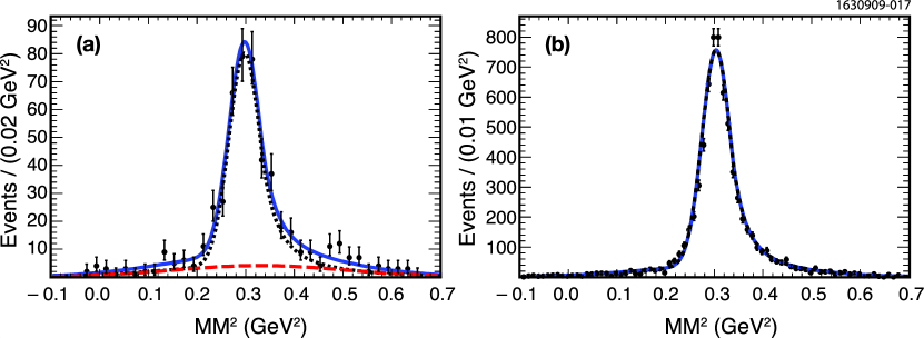
Figure 4: MM² spectrum of $\eta\pi^{+}\pi^{0}$, where $\eta\to\gamma\gamma$ was detected, but ignored in the calculation for both (a) data and (b) Monte Carlo events. The dotted line in (a) is the signal and the dashed line the background determined from the fit to the $D_{s}^{-}$ candidate invariant mass sidebands. The signal shapes are the sum of a Crystal Ball and Gaussian functions (see text).

In both the case of the Monte Carlo simulation and the data we fit the signal with the sum of Crystal Ball (CB) CBL and Gaussian functions. We fix some fit parameters that we find from the Monte Carlo simulation including the ratio of the r.m.s. widths ($\sigma$’s) for the Gaussian and CB functions, set to a value of 6, and the area of the Gaussian function with respect to the CB function to be 20%. In the data fit we also include the background given by the $D_{s}^{-}$ invariant mass sidebands. The CB function parameters $\alpha$ and $N$ are taken from the Monte Carlo simulation as 1 and 4.5, respectively. We find

$$\sigma_{\rm MC} = (0.0289\pm 0.0006)~{}{\rm GeV}^{2}~{}{\rm for~{}the~{}Monte~{}Carlo~{}CB~{}function,}$$ (4)

$$\sigma_{\rm Data} = (0.0320\pm 0.0020)~{}{\rm GeV}^{2}~{}{\rm for~{}the~{}data~{}CB~{}function,}$$

$$\sqrt{\sigma_{\rm Data}^{2}-\sigma_{\rm MC}^{2}} = (0.014\pm 0.005)~{}{\rm GeV}^{2}~{}.$$

We use the resolution as found in the data above when fitting the data for the $\eta\rho^{+}$ component and increase the width of the other narrow components.

III Signal Extraction

We proceed by preforming a simultaneous fit to the $D_{s}^{-}$ invariant mass, using a mass range within $\pm$70 MeV of the nominal mass and the MM². The procedure is similar to that used in Ref. Dstomunu . We first check our procedures by fitting the data MM² distribution in the $E_{\rm extra}$ interval above 0.8 GeV, where we have only background. We include the following decay modes as individual probability density functions (PDFs) in the fit: $K^{0}\pi^{+}\pi^{0}$, $\pi^{+}\pi^{0}\pi^{0}$, $\phi\pi^{+}$, $\eta\pi^{+}$, $\eta\rho^{+}$, $\eta^{\prime}\pi^{+}$, $\eta^{\prime}\pi^{+}\pi^{0}$, $\omega\pi^{+}\pi^{0}$. All narrow resonance structures are smeared by an additional r.m.s. resolution of 0.014 GeV², as determined by our $\eta\rho^{+}$ study (see section II.4). The other modes are lumped together into one other PDF. In the likelihood fit we add Gaussian constraints on the expected yields based on the known branching ratios and their errors.

The resulting fit to the data for 0.8 GeV $<~{}E_{\rm{extra}}$ is shown in Fig. 5. The fake $D_{s}^{-}$ background has been accounted for by simultaneously fitting the sidebands in $D_{s}^{-}$ invariant mass. The two-body modes show evident peaks and are well described by the fit, demonstrating that our understanding of the backgrounds appears to be adequate.

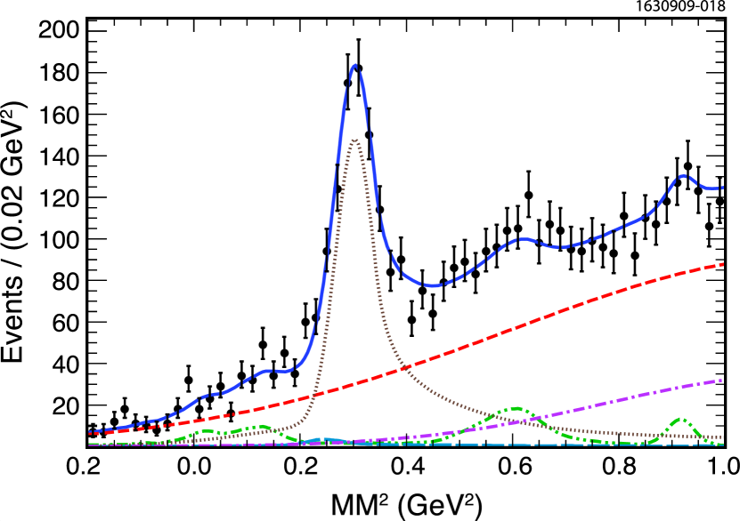
Figure 5: Fit to the data (points) for 0.8 GeV $<E_{\rm extra}$. The various components are $\eta\rho^{+}$ (dotted), fake $D_{s}^{-}$ (dashed), $K^{0}\pi^{+}\pi^{0}$ (long dash), sum of $\pi^{+}\pi^{0}\pi^{0}$, $\eta\pi^{+}$, $\omega\pi^{+}\pi^{0}$, $\phi\pi^{+}$, $\eta^{\prime}\pi^{+}$, and $\eta^{\prime}\pi^{+}\pi^{0}$ (dash-dot-dot), and other backgrounds (dashed-dot). The solid curve shows the total.

We next fit the two bins $E_{\rm extra}<0.1$ GeV and $0.1<E_{\rm extra}<0.2$ GeV separately. The background PDFs are shown in Figs. 6 and 7 for each interval. Note that they now include a separate PDF for $D_{s}^{+}\to\tau^{+}\nu$, where the $\tau^{+}$ decays into either $\pi^{+}\overline{\nu},~{}{\rm or}~{}\pi^{+}\pi^{0}\pi^{0}\overline{\nu}$. The fit projections for both intervals are shown in Figs. 8 and 9. For the first interval, $E_{\rm extra}<0.1$ GeV, the background level from all $D_{s}^{+}$ decays is about the same as that from fake $D_{s}^{-}$, and both are considerably smaller than the signal. For the second interval the signal and background levels are about equal. Table 1 summarizes the signal and background yields. (The notation “$\tau^{+}\to(\pi^{+}+\pi^{+}\pi^{0}\pi^{0})\overline{\nu}$” denotes the sum of two modes where $D_{s}^{+}\to\tau^{+}\nu$, and the $\tau^{+}$ decays to either $\pi^{+}\overline{\nu}$ or $\pi^{+}\pi^{0}\pi^{0}\overline{\nu}$.)

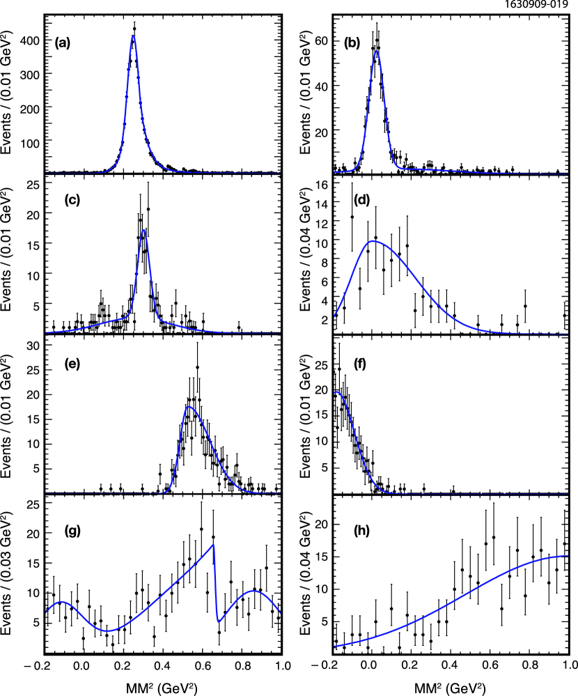
Figure 6: Fits to Monte Carlo simulation for the individual background PDFs for $E_{\rm extra}<$ 0.1 GeV, for the modes (a) $K^{0}\pi^{+}\pi^{0}$, (b) $\pi^{+}\pi^{0}\pi^{0}$, (c) $\eta\rho^{+}$, (d) $\eta\pi^{+}$, (e) $\phi\pi^{+}$, (f) $\mu^{+}\nu$, (g) $D_{s}^{+}\to\tau^{+}\nu$, $\tau^{+}\to(\pi^{+}+\pi^{+}\pi^{0}\pi^{0})\overline{\nu}$, (h) sum of the other small modes.

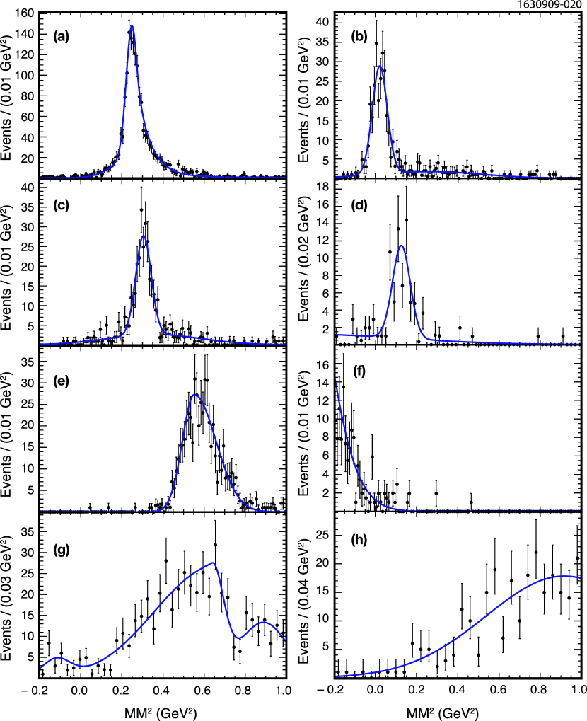
Figure 7: Fits to Monte Carlo simulation for the individual background PDFs for 0.1 $<E_{\rm extra}<$ 0.2 GeV, for the modes (a) $K^{0}\pi^{+}\pi^{0}$, (b) $\pi^{+}\pi^{0}\pi^{0}$, (c) $\eta\rho^{+}$, (d) $\eta\pi^{+}$, (e) $\phi\pi^{+}$, (f) $\mu^{+}\nu$, (g) $D_{s}^{+}\to\tau^{+}\nu$, $\tau^{+}\to(\pi^{+}+\pi^{+}\pi^{0}\pi^{0})\overline{\nu}$, (h) sum of the other small modes.

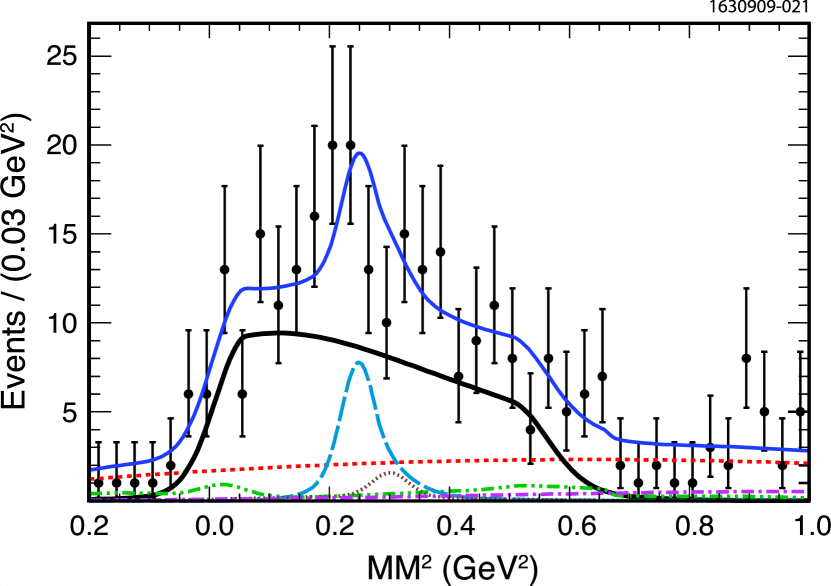
Figure 8: Fit to the data (points) for $E_{\rm extra}<$ 0.1 GeV. The various components are signal (thick solid line), $\eta\rho^{+}$ (dotted), fake $D_{s}^{-}$ (dashed), $K^{0}\pi^{+}\pi^{0}$ (long dash), sum of $\pi^{+}\pi^{0}\pi^{0}$, $\eta\pi^{+}$, $\phi\pi^{+}$, $\tau^{+}\to(\pi^{+}+\pi^{+}\pi^{0}\pi^{0})\overline{\nu}$, $\mu^{+}\nu$, and $X\mu^{+}\nu$ (dash-dot-dot), and other backgrounds (dashed-dot). The thinner solid curve shows the total.

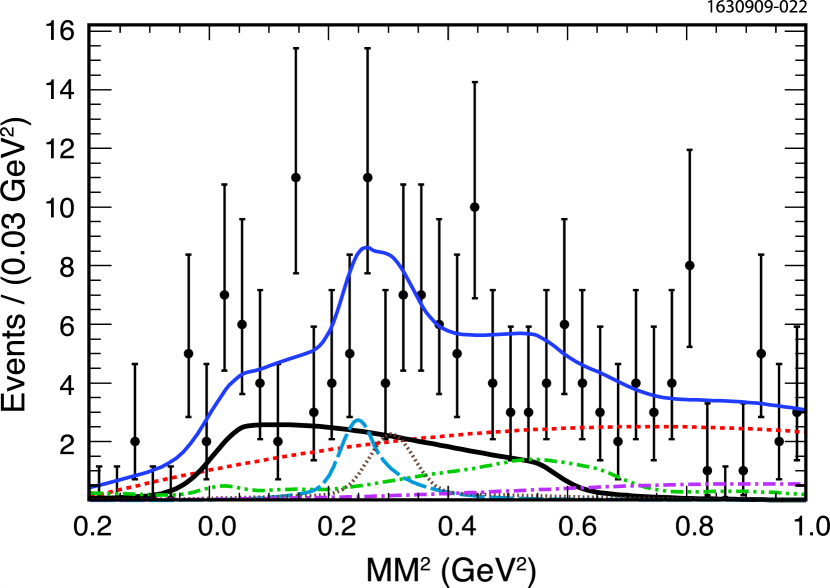
Figure 9: Fit to the data (points) for $0.1~{}<E_{\rm extra}<$ 0.2 GeV. The various components are signal (thick solid line), $\eta\rho^{+}$ (dotted), fake $D_{s}^{-}$ (dashed), $K^{0}\pi^{+}\pi^{0}$ (long dash), sum of $\pi^{+}\pi^{0}\pi^{0}$, $\eta\pi^{+}$, $\phi\pi^{+}$, $\tau^{+}\to(\pi^{+}+\pi^{+}\pi^{0}\pi^{0})\overline{\nu}$, $\mu^{+}\nu$, and $X\mu^{+}\nu$ (dash-dot-dot), and other backgrounds (dashed-dot). The thinner solid curve shows the total.

Table 1: Signal and background yields from the fit in two $E_{\rm extra}$ intervals. We also list the measured or assumed background branching fractions and the r.m.s. error on the fit constraint resulting either from the branching fraction error or other considerations. The # MC indicates the predicted background number of events for the assumed branching ratio input as the starting point of the fit, while # Data gives the number determined by the fit.

Component	${\cal B}$(%)	Constraint	$E_{\rm extra}<0.1$ GeV		$0.1<E_{\rm extra}<0.2$ GeV
		Error (%)	# MC	# Data	# MC	# Data
Signal				155.2$\pm$16.5		43.7$\pm$11.3
$K^{0}\pi^{+}\pi^{0}$	1.0$\pm$0.2	20	26.1	25.2$\pm$4.8	11.0	10.5$\pm$2.1
$\eta\rho^{+}$	$8.9\pm 0.7$	4.2	7.1	7.0$\pm$0.6	10.6	10.5$\pm$0.9
$\pi^{+}\pi^{0}\pi^{0}$	$0.65\pm 0.14$	22	2.8	$2.8\pm 0.6$	1.5	$1.6\pm 0.3$
$\tau^{+}\to(\pi^{+}+\pi^{+}\pi^{0}\pi^{0})\overline{\nu}$	$1.14\pm 0.06$	25†	8.5	$8.4\pm 2.1$	12.2	$10.9\pm 3.0$
$\mu^{+}\nu$	$0.576\pm 0.045$	5.4	1.0	$1.0\pm 0.1$	0.48	$0.5\pm 0.1$
$\eta\pi^{+}$	$1.58\pm 0.21$	13.3	0.9	$0.9\pm 0.1$	0.9	$0.9\pm 0.1$
$\phi\pi^{+}$	$4.35\pm 0.35$	8	1.7	$1.7\pm 0.2$	2.8	$2.8\pm 0.3$
$X\mu^{+}\nu$	5.9	35‡	3.4	$3.4\pm 1.2$	7.4	$6.6\pm 2.6$
Other background		$30^{*}$	11.5	$11.4\pm 3.3$	11.8	$10.5\pm 3.3$
Fake $D_{s}^{-}$ background				$81.8\pm 5.0$		$74.8\pm 4.6$
$\dagger$ The error is based on the uncertainties of the resonant substructure that can alter the efficiency.
$\ddagger$ We assign a 35% uncertainty based upon the error on ${\cal{B}}(D_{s}^{+}\to Xe^{+}\nu)$.
$*$ We assign a 30% uncertainty based on the sample size.

Adding the signal yields in the two $E_{\rm extra}$ intervals, taking into account the efficiency for finding the $\rho^{+}$ in each interval, and dividing by the number of $D_{s}^{-}$ tags (43859$\pm$936$\pm$877) we find

$${\cal B}(D_{s}^{+}\to\tau^{+}\nu)=(5.52\pm 0.57\pm 0.21)\%,$$ (5)

where the first error is statistical and the second systematic. We will discuss the systematic errors in the next section. In the smallest $E_{\rm extra}$ interval the branching fractions is $(5.48\pm 0.59)$%, while in the higher interval it is $(5.65\pm 1.47)$%. The numbers are consistent. We note the data including the background components is well-modeled in all three $E_{\rm extra}$ intervals, confirming our understanding of the background.

III.1 Systematic Errors

The sources of systematic errors in the branching fraction are listed in Table 2. As we have let the branching fractions of the background components float in the fit by their known errors, there is no additional contribution from this source. The systematic error in the background is estimated using two different techniques. First of all, if we remove the Gaussian constraint on the sum of the other small mode background fractions we observe a 1.1% increase in the signal yield. Secondly, if we change the parameters of the background shape containing the sum of the other small modes the yield decreases by 0.5%. A separate source of error is the efficiency on the detection of background events; if we change the $E_{\rm extra}$ efficiency and the $\pi^{0}$ efficiency by their errors, and thus change the background yields, we observe a combined error of $\pm$1.1%. An additional systematic error could arise from Cabibbo suppressed $\tau^{+}\to K^{+}\pi^{0}\overline{\nu}$ decays. The measured branching fraction for these decays is 1.6% of that of $\pi^{+}\pi^{0}\overline{\nu}$. The combination of $dE/dx$ and RICH particle identification reduces the kaon yield by more than 95%, resulting in a negligible $<0.1$% contamination.

Table 2: Systematic errors on determination of the branching fraction.

Error Source	Size (%)
Finding the $\pi^{+}$ track from the $\rho^{+}$ decay	0.3
Hadron identification	1.0
Finding the $\pi^{0}$ from the $\rho^{+}$ decay	1.3
$E_{\rm extra}<$ 0.2 GeV & $\pi^{0}$ efficiencies on background	1.1
$E_{\rm extra}<$ 0.2 GeV signal efficiency	2.0
Background modeling	1.1
Number of tags	2.0
Tag bias	1.0
Total	3.8

Since we are requiring that $E_{\rm extra}$ be below either 0.1 or 0.2 GeV, it is necessary to check this efficiency in the data. Our procedure is to use the fully reconstructed sample of $e^{+}e^{-}\to D_{s}D_{s}^{*}$ events selected the same way as described in Ref. Dstomunu . The $E_{\rm extra}$ distributions from Monte Carlo simulation and data for this sample are shown in Fig. 10. The agreement with the simulation is excellent. Table 3 gives the efficiency from Monte Carlo simulation for our double tag sample and the efficiency measured in the data for specific ranges in $E_{\rm extra}$. The situation here corresponds to the extra energy deposited by two tags. We need to translate these numbers to the case of one tag plus a signal $\rho^{+}$. A cut at $E_{\rm extra}=0.3$ GeV in the double tag data corresponds to the same efficiency as a cut of 0.2 GeV in the single tag plus $\rho^{+}$ data. The difference between Monte Carlo simulation and data then is $(-1.2\pm 1.6)$%, which implies a systematic error of $\pm$2.0% in this efficiency.

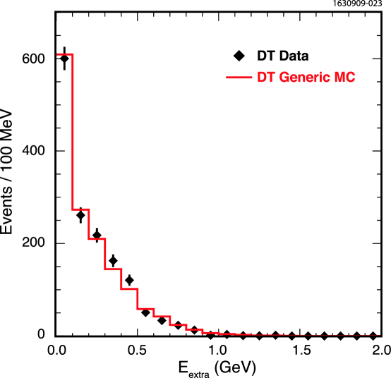
Figure 10: The $E_{\rm extra}$ distributions from $e^{+}e^{-}\to D_{s}^{*}D_{s}$ events with both $D_{s}$ decays fully reconstructed (DT) for data (diamond) and Monte Carlo simulation (histogram).

Table 3: The efficiencies ($\epsilon$) for Data and Monte Carlo simulation for different requirements on $E_{\rm extra}$, and the corresponding fractional differences.

$E_{\rm extra}$ (GeV)	$\epsilon_{\rm Data}$(%)	$\epsilon_{\rm MC}$(%)	$\epsilon_{\rm Data}/\epsilon_{\rm MC}-1$ (%)
$<$0.1	$40.24\pm 1.27$	$40.81\pm 0.31$	$-1.4\pm 3.2$
$<$0.2	$57.75\pm 1.28$	$59.12\pm 0.31$	$-2.3\pm 2.2$
$<$0.3	$72.35\pm 1.16$	$73.21\pm 0.28$	$-1.2\pm 1.6$
$<$0.4	$83.27\pm 0.97$	$82.91\pm 0.24$	$0.4\pm 1.2$

We note that if we fix the background branching fractions to their nominal values, and refit the data, the statistical error in the $E_{\rm extra}<$ 0.1 GeV bin decreases from 16.5 to 15.9 events, and in the 0.1 $<E_{\rm extra}<$ 0.2 GeV bin decreases from 11.3 to 11.1 events. Thus, our statistical error contains a significant component from the background estimates.

III.2 Cross Checks Using $\pi^{+}\pi^{0}$ Helicity and Mass Distributions

In principle the best way to view the $\rho^{+}$ polarization is to look at the angle $\theta$ of the $\pi^{+}$ with respect to the $\rho^{+}$ direction in the $\tau^{+}$ rest frame. Since we cannot reconstruct the $\tau^{+}$, we use the laboratory frame. We consider all events in the $E_{\rm extra}$ interval below 0.2 GeV and having $-0.05~{}<$MM${}^{2}~{}<$ 0.60 GeV². Fig. 11 shows $\cos\theta$ from the data with sidebands subtracted compared with the sum of expected signal and backgrounds from Monte Carlo simulation, normalized by yields from the data fit. The predicted total is in good agreement with the shape and data yield.

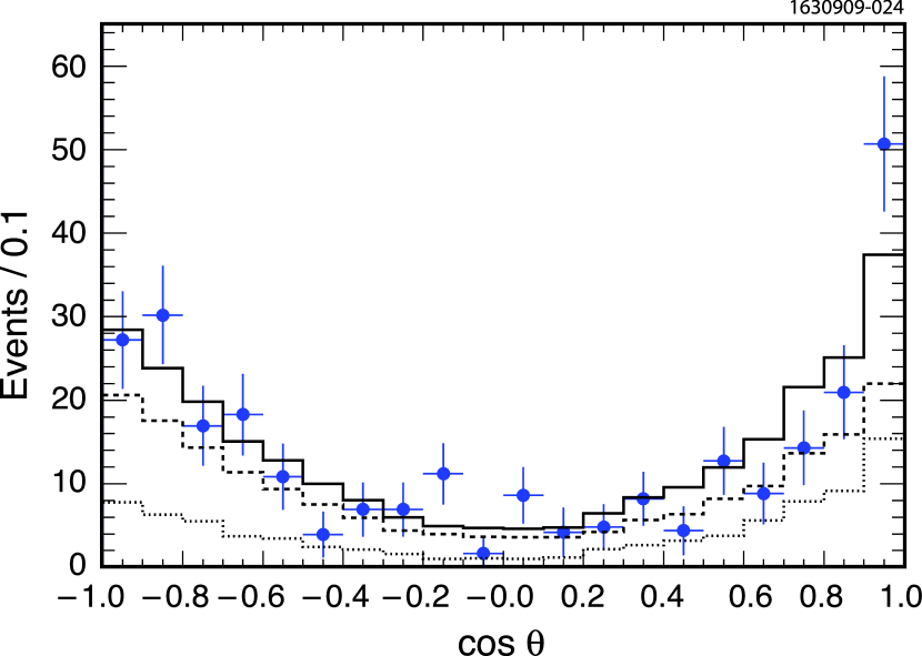
Figure 11: Helicity distribution from the $\rho^{+}$ decay as measured in the laboratory frame. The points with error bars are the sideband subtracted data. The dashed line represents the predicted signal shape and the dotted line the predicted background shape from real $D_{s}^{+}$ decays. The Monte Carlo predictions are normalized by the fitted yields to the data. The predicted total is given by the solid line. We require that $E_{\rm extra}~{}<$ 0.2 GeV, and $-0.05~{}<$MM${}^{2}~{}<$ 0.60 GeV².

We also show the $\pi^{+}\pi^{0}$ mass distribution in Fig. 12. Again the predicted sum has good agreement with the shape and data yield.

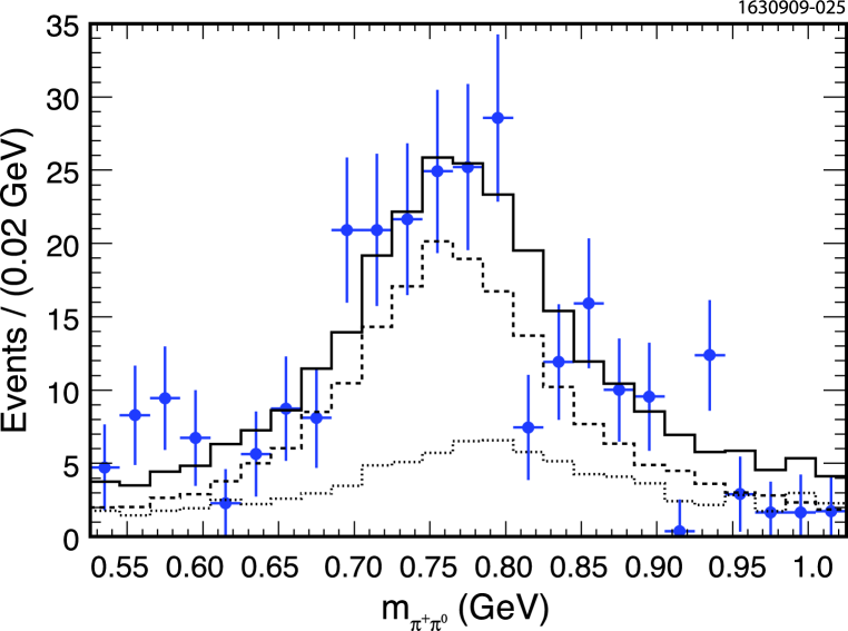
Figure 12: Distribution of $\pi^{+}\pi^{0}$ mass. The points with error bars are the sideband subtracted data. The dashed line represents the Monte Carlo predicted signal shape and the dotted line the Monte Carlo predicted background shape from real $D_{s}^{+}$ decays. The Monte Carlo predictions are normalized by the fitted yields to the data. The predicted total is given by the solid line. We require that $E_{\rm extra}~{}<$ 0.2 GeV, and $-0.05~{}<$MM${}^{2}~{}<$ 0.60 GeV².

IV Conclusions

We list the CLEO-c measurements of leptonic branching ratios and $f_{D_{s}}$ in Table 4. To extract the decay constant we use $M_{D_{s}^{+}}=1.96849(34)$ GeV, a $D_{s}^{+}$ lifetime of 0.500(7) ps, and 1.77684(17) GeV for the $\tau^{+}$ mass PDG . While it has been customary to take $|V_{cs}|=|V_{ud}|$, the expansion of the Wolfenstein parametrization of the CKM matrix to order $\lambda^{4}$ Charles implies that $|V_{cs}|=|V_{ud}|-|V_{cb}|^{2}/2$. We use $|V_{ud}|=0.97418(26)$ as derived in Ref. Towner-Hardy . For $|V_{cb}|$ we use a value of 0.04 from an average of exclusive and inclusive semileptonic $B$ decay results as discussed in Ref. ABS . Thus, we find $|V_{cs}|=0.97338(26)$. The resulting value of $f_{D_{s}}$ is 0.2 MeV larger than taking $|V_{cs}|=|V_{ud}|$.

Previously reported values of $f_{D_{s}}$ have been corrected to corresponded to the above numbers. These quantities contribute additional small amounts to the systematic error of $\pm$1.8 MeV (lifetime), $\pm$0.1 MeV ($V_{cs}$), and for the $\tau^{+}\nu$ mode only $\pm$0.4 MeV ($M_{D_{s}^{+}}$) and $\pm 0.2$ MeV ($\tau^{+}$ mass), that are included in the quoted values. A theoretical upper bound on $f_{D_{s}}$ of 270 MeV has been calculated using two-point correlation functions by Khodjamirian Kho . The CLEO-c values for both the $\tau^{+}\nu$ and $\mu^{+}\nu$ modes are below this limit.

Table 4: Recent absolute measurements of $f_{D_{s}}$ from CLEO-c

. Experiment Mode ${\cal B}$ (%) $f_{D_{s}}$ (MeV) This result $\tau^{+}\nu~{}(\rho^{+}\overline{\nu})$ $(5.52\pm 0.57\pm 0.21)$ $257.8\pm 13.3\pm 5.2$ CLEO-c Dstomunu $\tau^{+}\nu,~{}(\pi^{+}\overline{\nu})$ $(6.42\pm 0.81\pm 0.18)$ $278.0\pm 17.5\pm 4.4$ CLEO-c CLEO-CSP $\tau^{+}\nu~{}(e^{+}\nu\overline{\nu})$ $(5.30\pm 0.47\pm 0.22)$ $252.6\pm 11.2\pm 5.6$ Average $\tau^{+}\nu$ $(5.58\pm 0.33\pm 0.13)$ $259.7\pm 7.8\pm 3.4$ CLEO-c Dstomunu $\mu^{+}\nu$ $(0.565\pm 0.045\pm 0.017)$ $257.6\pm 10.3\pm 4.3$ Average $\tau^{+}\nu$+$\mu^{+}\nu$ $259.0\pm 6.2\pm 3.0$

The ratio of decay constants from CLEO for the two leptonic decay modes is

$$\frac{f_{D_{s}}\left(D_{s}^{+}\to\tau^{+}\nu\right)}{f_{D_{s}}\left(D_{s}^{+}\to\mu^{+}\nu\right)}=1.01\pm 0.05,$$ (6)

consistent with lepton universality. The average value of the pseudoscalar decay constant using both leptonic decay modes is

$$f_{D_{s}}=(259.0\pm 6.2\pm 3.0){\rm~{}MeV}.$$ (7)

There are two SM based theoretical predictions for $f_{D_{s}}$ in the literature based on Lattice QCD calculations, where all three light quark loops are included. The values predicted are ($241\pm 3$) MeV from the HPQCD+UKQCD collaboration Lat:Foll , and ($249\pm 11$) MeV from the FNAL+MILC+HPQCD collaboration Lat:Milc . We choose to compare with the more precise Follana et al. result, realizing that it needs confirmation, especially with respect to the rather small error. The difference between the experimental average of $f_{D_{s}}$ and the HPQCD+UKQCD prediction is 2.4 standard deviations. Other theoretical predictions are given in Ref. Rosner-Stone .

Belle has also measured the absolute branching fraction for $D_{s}^{+}\to\mu^{+}\nu$ and found a value $f_{D_{s}}=(275\pm 16\pm 12)$ MeV Belle-munu ; Otherfds . Combining with the CLEO measurements we find $f_{D_{s}}=(260.7\pm 6.5$) MeV, which differs from the HPQCD+UKQCD prediction by 2.8 standard deviations. We emphasize that this difference is qualitatively different than looking for new physics as a bump in mass spectrum where any values of the mass and width can be entertained. Here we are dealing with a theoretical number that was predicted before the measurements were available. Thus, although we cannot claim to have definitely seen an important discrepancy pointing to physics beyond the standard model, it is important to pay attention to this difference and to see what it may imply.

In fact this possible discrepancy has motivated several new beyond the SM theories. These include leptoquark models of Dobrescu and Kronfeld Dobrescu-Kronfeld , R parity violating models of Akeroyd and Recksiegel Rviolating , and Kundu and Nandi who relate this discrepancy with preliminary indications of a large phase in $B_{s}-\overline{B}_{s}$ mixing, and explain both with a specific supersymmetry model KN . Dosner et al. Dosner show however, that scalar leptoquark and R-parity violating models would have different effects on $\tau^{+}\nu$ and $\mu^{+}\nu$ final states. Gninenko and Gorbunov argue that the neutrino in the $D_{s}$ decay mixes with a sterile neutrino, which enhances the rate and also explains the excess number of low energy electron like events in the MiniBooNE data GG .

We also have measured the following branching fractions:

$${\cal B}(D_{s}^{+}\to K^{0}\pi^{+}\pi^{0}) = (1.00\pm 0.18\pm 0.04)\%,$$ (8)

$${\cal B}(D_{s}^{+}\to\pi^{+}\pi^{0}\pi^{0}) = (0.65\pm 0.13\pm 0.03)\%,$$

$${\cal B}(D_{s}^{+}\to\eta\rho^{+}) = (8.9\pm 0.6\pm 0.5)\%.$$

The first two modes have not been measured previously.

V Acknowledgments

We thank Nabil Menaa for useful discussions. We gratefully acknowledge the effort of the CESR staff in providing us with excellent luminosity and running conditions. D. Cronin-Hennessy and A. Ryd thank the A.P. Sloan Foundation. This work was supported by the National Science Foundation, the U.S. Department of Energy, the Natural Sciences and Engineering Research Council of Canada, and the U.K. Science and Technology Facilities Council.

Appendix A: Monte Carlo Generated Background Modes

We list the different modes that populate the MM² distribution for the three $E_{\rm extra}$ intervals as given by the generic Monte Carlo simulation in Table 5.

Table 5: Assumed branching fractions, Numbers of events (#) and fractions resulting from a generic Monte Carlo simulation of the $D_{s}^{+}$ backgrounds for twenty times the data in the interval $-0.2<$ MM${}^{2}<1.0$ GeV².

Mode	${\cal B}$(%)	$0<E_{\rm extra}<0.1$ GeV		$0.1<E_{\rm extra}<0.2$ GeV		0.8 GeV $<E_{\rm extra}$
		#	Fraction (%)	#	Fraction (%)	#	Fraction (%)
$K^{0}\pi^{+}\pi^{0}$	0.85	348	29.3	128	10.3	548	1.61
$\eta\rho^{+}$	7.58	114	9.6	215	17.4	17797	52.4
$\pi^{+}\pi^{0}\pi^{0}$	0.58	48	4.1	27	2.2	991	2.9
$\tau^{+}\nu$, $\tau^{+}\to\pi^{+}\pi^{0}\pi^{0}\bar{\nu}$	0.55	159	13.4	266	21.5	99	0.3
$\tau^{+}\nu$, $\tau^{+}\to\pi^{+}\bar{\nu}$	0.66	63	5.3	18	1.5	2	0.01
$\tau^{+}\nu$, $\tau^{+}\to$ other	3.27	81	6.8	43	3.5	12	0.04
$\phi\pi^{+}$, $\phi\to K_{L}^{0}K_{S}^{0}$	1.38	70	5.9	114	9.2	560	1.7
$X\mu^{+}\nu$	5.87	91	7.7	158	12.8	653	1.9
$\eta\pi^{+}$	1.54	15	1.3	32	2.6	1250	3.7
$\mu^{+}\nu$	0.61	19	1.6	15	1.2	9	0.03
$\eta^{\prime}\pi^{+}$	3.67	10	0.84	15	1.2	2610	7.7
$K^{0}K^{+}\pi^{0}$	2.50	20	1.7	7	0.6	32	0.09
$K^{0}K^{+}$	2.93	11	0.9	6	0.5	31	0.09
$K^{0}\pi^{+}$	0.24	9	0.8	9	0.7	59	0.17
$K_{S}^{0}K_{S}^{0}\pi^{+}$	0.70	0	0	1	0.1	156	0.46
$K_{S}^{0}K_{L}^{0}\pi^{+}$	1.25	29	2.5	62	5.0	144	0.42
$K_{L}^{0}K_{L}^{0}\pi^{+}$	0.70	18	1.5	8	0.7	31	0.09
$Xe^{+}\nu$	6.19	8	0.7	5	0.4	16	0.05
$K^{0}\pi^{+}\pi^{0}\pi^{0}$	0.65	24	2.0	47	3.8	457	1.34
$\eta\pi^{+}\pi^{0}\pi^{0}$	3.25	5	0.4	12	1.0	4357	12.82
$\eta^{\prime}\pi^{+}\pi^{0}$	3.87	2	0.2	6	0.5	2041	6.00
$\omega\pi^{+}$	0.25	1	0.1	0	0	18	0.05
$\pi^{+}\pi^{0}\pi^{0}\pi^{0}\pi^{0}$	0.85	1	0.1	3	0.2	1684	4.95
$\phi\pi^{+}\pi^{0}$	7.35	4	0.3	14	1.1	340	1.00
Other		36	3.0	27	2.2	97	0.29

Appendix B: Measurements of $D_{s}^{+}$ Branching Fractions for Selected Background Modes

The $K^{0}\pi^{+}\pi^{0}$ mode has not been previously measured. We select events opposite our $D_{s}^{-}$ tag candidates with a single charged track consistent with being a $\pi^{+}$ in conjunction with a $\pi^{0}$ candidate as described above, and a $K_{S}^{0}\to\pi^{+}\pi^{-}$ candidate where the invariant $\pi^{+}\pi^{-}$ mass is within 12 MeV of the known $K_{S}^{0}$ mass and the flight significance, the distance that the $K_{S}$ travels divided by the error in the distance, is greater than 2. The invariant mass of $K_{S}^{0}\pi^{+}\pi^{0}$ combinations is shown in Fig. 13. The data are fit with a signal CB function with all parameters except the area fixed to those given by the Monte Carlo simulation of this mode, and a second order Chebyshev background polynomial. The fit yields 44$\pm$8 events.

We proceed by performing an unbinned liklihood fit to the Daltiz plot shown in Fig. 14, using the isobar model formalism as described in Ref. isobar . The fit results are that the $K_{S}^{0}\rho^{+}$ fraction is (88$\pm$8)% with only (17$\pm$8)% of $K^{*+}\pi^{0}$; the relative phase is (21$\pm$25) degrees. The efficiency is determined to be 21% by Monte Carlo simulation which uses a $K\rho$ resonance structure, resulting in a branching fraction

$${\cal B}(D_{s}^{+}\to K^{0}\pi^{+}\pi^{0})=(1.00\pm 0.18\pm 0.04)\%,$$ (9)

where the systematic error arises from several sources shown in Table 6. The error due to the Dalitz plot structure is is 0.7%, found by evaluating the relative efficiency difference between pure $K_{S}\rho^{+}$ and the model resulting from our Dalitz plot fit; this is negligible compared to the other sources. Note that for our purposes some of the systematic error cancels because we are using the same $D_{s}^{-}$ tag sample and the same $\pi^{+}$ and $\pi^{0}$ detection efficiencies as for signal $\tau^{+}\to\rho^{+}\overline{\nu}$.

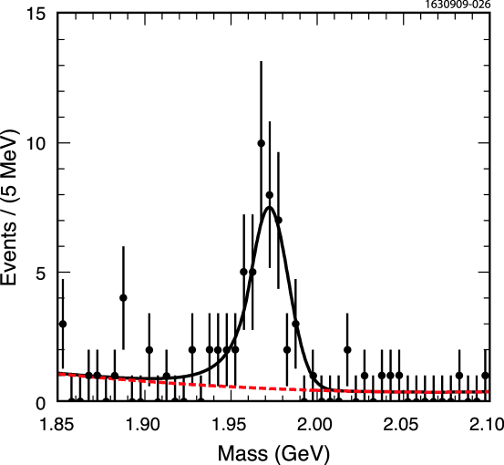
Figure 13: The invariant mass spectrum of $K_{S}^{0}\pi^{+}\pi^{0}$. The curves show a second order Chebyshev polynomial function that describes the background summed with a signal CB function whose width is fixed (solid line).

Figure 14: (a) Dalitz plot of $K_{S}^{0}\pi^{+}\pi^{0}$, where the invariant mass of the three particles is selected within $\pm$20 MeV of the $D_{s}^{+}$ mass. (b)–(d) show the mass projections, the solid curves show the overall fit and the dashed curve the background from sidebands.

Table 6: Systematic errors on determination of the branching fractions of several background modes. We give two errors, one for the branching fraction to be used as an independent measurement (Ext), and the second is the one to be used internally (Int) for the lepton branching fraction analysis where some of the errors cancel.

	$D_{s}^{+}\to K^{0}\pi^{+}\pi^{0}$		$D_{s}^{+}\to\eta\rho^{+}$		$D_{s}^{+}\to\pi^{+}\pi^{0}\pi^{0}$
Error Source	(Ext)(%)	(Int)(%)	(Ext)(%)	(Int)(%)	(Ext)(%)	(Int)(%)
Hadron identification	1.0	0	1.0	0	1.0	0
Finding $\pi^{0}$ from ($\rho^{+}$)	1.3	0	1.3	0	1.3	0
Background modeling	2.0	2.0	1.9	1.9	2.0	2.0
$\pi^{0}$ efficiency	1.3	0	1.3	0	2.6	1.3
$K^{0}$ efficiency	2.0	2.0	0	0	0	0
$\eta$ efficiency	0	0	4.0	4.0	0	0
Number of tags	2.0	0	2.0	0	2.0	0
Tag bias	1.0	0	1.0	0	1.0	0
Total	3.8	2.8	5.1	4.4	4.0	2.4

The $\pi^{+}\pi^{0}\pi^{0}$ mode also has not previously been measured, though the analogous isospin related mode $\pi^{+}\pi^{+}\pi^{-}$ has been. Here we require that the invariant $\pi^{0}\pi^{0}$ mass be more than 50 MeV from the $K_{S}^{0}$ mass in order to reject $K_{S}^{0}$. The invariant mass plot is shown in Fig. 15. The signal CB function is fixed to the Monte Carlo predicted shape, and we use a second order Chebyshev polynomial function to model the background shape. We find a signal of $72\pm 16$ events.

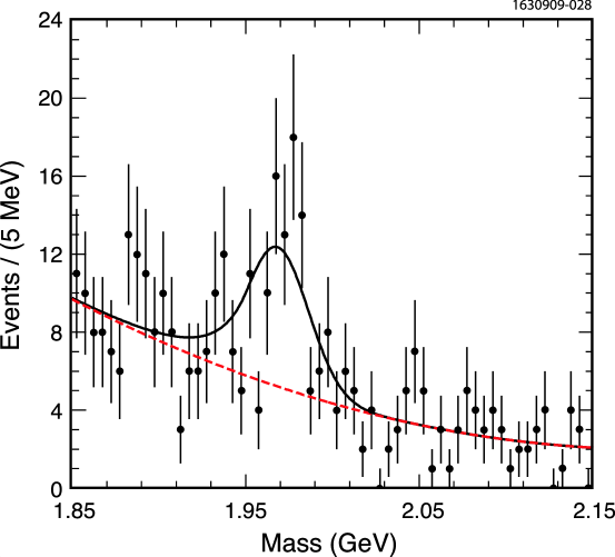
Figure 15: The invariant mass spectrum of $\pi^{+}\pi^{0}\pi^{0}$ candidates. The curves show a second order Chebyshev polynomial function that describes the background (dashed line) summed with signal CB function (solid line) whose width is fixed to the Monte Carlo predicted shape plus the measured Gaussian smearing.

We also perform an unbinned liklihood fit to the Daltiz plot shown in Fig. 16, again using the isobar model formalism. There is no evidence for $\rho^{+}\pi^{0}$. We find that the fractions of $f_{0}(980)\pi^{+}$, $f_{2}(1270)\pi^{+}$ and $f_{0}(1370)\pi^{+}$ are (56.5$\pm$9.1)%, (20.5$\pm$7.3)%, and (38.1$\pm$8.6)%, respectively. Fixing the $f_{0}(980)\pi^{+}$ phase at zero degrees, the relative phases of the $f_{2}(1270)\pi^{+}$ and $f_{0}(1370)\pi^{+}$ with respect to zero are (243$\pm$29) degrees and (299$\pm$24) degrees, respectively.

Figure 16: (a) Dalitz plot of $\pi^{+}\pi^{0}\pi^{0}$, where the invariant mass of the three particles is selected within $\pm$24 MeV of the $D_{s}^{+}$ mass. There are two entries per event. (b)–(d) show the mass projections, the solid curves show the overall fit and the shaded region the background from sidebands. The zero at 0.25 GeV² in (d) results from the $K_{S}$ rejection criteria.

The Monte Carlo simulated efficiency is 28.1%, yielding

$${\cal B}(D_{s}^{+}\to\pi^{+}\pi^{0}\pi^{0})=(0.65\pm 0.13\pm 0.03)\%.$$ (10)

The systematic errors are listed in Table 6. This number is consistent with ${\cal B}(\pi^{+}\pi^{+}\pi^{-})/2=(0.56\pm 0.04)$% PDG , which is what is expected if the neutral dipion system final state dominates both modes.

The $\eta\rho^{+}$ branching fraction has been previously measured as ($13.1\pm 2.2)$% PDG ; we wish to improve on this accuracy. We look for events with only one charged track consistent with being a $\pi^{+}$ The $\eta$ is looked for in the $\gamma\gamma$ decay mode only; mass combinations are used if they are within 3 standard deviations of the $\eta$ mass. We insist that the $\pi^{+}\pi^{0}$ invariant mass be within 250 MeV of the $\rho^{+}$ mass. The resulting $\gamma\gamma\pi^{+}\pi^{0}$ invariant mass spectrum is shown in Fig. 17. Here we have enough data to let the r.m.s. width of the CB function vary in the fit. The background is again described by a second order Chebyshev function. We find a total of $328\pm 22$ events. We use a Monte Carlo determined efficiency of 22.4%. We find that

$${\cal B}(D_{s}^{+}\to\eta\rho^{+})=(8.9\pm 0.6\pm 0.5)\%.$$ (11)

The systematic errors are listed in Table 6. Our new measurement is lower by about 1.8 standard deviations than the PDG average PDG .

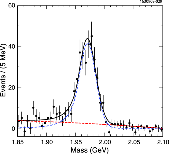
Figure 17: The invariant mass spectrum of $\eta\pi^{+}\pi^{0}$ candidates, where $\eta\to\gamma\gamma$. The curves show a signal CB function whose width is allowed to float (dotted line), a second order Chebyshev polynomial function that describes the background (dashed line), and the sum (solid line).

References

(1)
D. Silverman and H. Yao, Phys. Rev. D 38, 214 (1988).
(2)
E. Follana, C. T. H. Davies, G. P. Lepage, and J. Shigemitsu (HPQCD and UKQCD Collaborations), Phys. Rev. Lett. 100, 062002 (2008), arXiv:0706.1726 [hep-lat].
(3)
J. L. Rosner and S. Stone in Ref. PDG , see also arXiv:0802.1043 [hep-ex].
(4)
C. Amsler et al. (Particle Data Group), Physics Letters B 667, 1 (2008).
(5)
A.G. Akeroyd and F. Mahmoudi, JHEP 0904, 121 (2009), arXiv:0902.2393 [hep-ph].
(6)
D. Peterson et al., Nucl. Instrum. and Methods A 478, 142 (2002);
Y. Kubota et al. (CLEO Collaboration), Nucl. Instrum. and Methods A 320, 66 (1992).
(7)
M. Artuso et al., Nucl. Instrum. Methods A 554, 147 (2005)
[physics/0506132].
(8)
D. Cronin-Hennessy et al. (CLEO Collaboration), Phys. Rev. D 80, 072001, (2009),
arXiv:0801.3418 [hep-ex].
(9)
J. P. Alexander et al. (CLEO Collaboration), Phys. Rev. D 79, 052001 (2009), arXiv:0901.1216 [hep-ex].
(10)
M. Fujikawa et al. (Belle Collaboration), Phys. Rev. D 78, 072006 (2008), arXiv:0805.3773 [hep-ex].
(11)
G. Bonvicini et al. (CLEO Collaboration), Phys. Rev. D 70, 112004 (2004), arXiv:hep-ex/0411050.
(12)
T. Skwarnicki, DESY F31-86-02
(thesis, unpublished) (1986).
(13)
J. Charles et al. Eur. Phys. J. C 41, 1 (2005), arXiv:hep-ph/0406184.
(14)
I. S. Towner and J. C. Hardy, Phys. Rev. C 77, 025501 (2008) arXiv:0710.3181 [nucl-th].
(15)
M. Artuso, E. Barberio and S. Stone, PMC Physics A, 3:3 (2009) arXiv:0902.3743 [hep-ph].
(16) P.U.E. Onyisi et al. (CLEO Collaboration),
Phys. Rev. D 79, 052002 (2009), arXiv:0901.1147 [hep-ex].
(17)
A. Khodjamirian, Phys. Rev. D 79, 031503(R) (2009) arXiv:0812.3747 [hep-ph].
(18)
C. Bernard et al. (Fermilab Lattice, MILC and HPQCD Collaborations),
arXiv:904.1895 [hep-lat] (2009); C. Aubin et al., Phys. Rev. Lett. 95, 122002 (2005), arXiv:hep-lat/0506030.
(19) L. Widhalm et al. (Belle Collaboration),
Phys. Rev. Lett. 100, 241801 (2008), arXiv:0709.1340 [hep-ex].
(20)
We have not included other measurements of in the average that are based on measuring the
leptonic branching fractions with respect to a hadronic decay mode due to the relatively large uncertainities
in the determination of the relevant hadronic branching fraction. See Ref. Rosner-Stone for a compilation
of these results.
(21)
B. A. Dobrescu and A. S. Kronfeld, Phys. Rev. Lett. 100, 241802 (2008), arXiv:0803.0512 [hep-ph].
(22)
An example of such a model is R-parity violating SUSY; see
A. G. Akeroyd and S. Recksiegel, Phys. Lett. B. 554, 38 (2003),
hep-ph/0210376.
(23)
A. Kundu and S. Nandi, Phys. Rev. D 78, 015009 (2008), arXiv:0803.1898 [hep-ph].
(24)
I. Dorsner, S. Fajfer, J. F. Kamenik, and N. Kosnik, arXiv:0906.5585 [hep-ph].
(25)
S. N. Gninenko and D. S. Gorbunov, arXiv:0907.4666 [hep-ph] (2009).
(26)
S. Kopp et al. (CLEO Collaboration), Phys. Rev. D 63, 092001 (2001); P. Rubin etal (CLEO Collaboration), Phys. Rev. D 78, 072003 (2008).