Nitrogen K-shell photoabsorption

Abstract

Reliable atomic data have been computed for the spectral modeling of the nitrogen K lines, which may lead to useful astrophysical diagnostics. Data sets comprise valence and K-vacancy level energies, wavelengths, Einstein $A$-coefficients, radiative and Auger widths and K-edge photoionization cross sections. An important issue is the lack of measurements which are usually employed to fine-tune calculations so as to attain spectroscopic accuracy. In order to estimate data quality, several atomic structure codes are used and extensive comparisons with previous theoretical data have been carried out. In the calculation of K photoabsorption with the Breit–Pauli $R$-matrix method, both radiation and Auger damping, which cause the smearing of the K edge, are taken into account. This work is part of a wider project to compute atomic data in the X-ray regime to be included in the database of the popular xstar modeling code.

1 Introduction

The improved resolution and sensitivity of current satellite-borne X-ray observatories (Chandra and XMM Newton) are allowing the study of previously inaccessible weak spectral features of astrophysical interest. In the early stages of these missions, it was realized that absorption by near-neutral species was common, and the fact that all charge states (except the fully ionized) left identifiable imprints in the X-ray spectrum has proven to be a powerful diagnostic. Inner-shell absorption is important in the outflows of Seyfert galaxies in terms of both Fe L$\alpha$ (Sako et al., 2001; Behar et al., 2001) and K$\alpha$ lines of high-Z elements (Behar & Netzer, 2002), and also of elements in the first row of the periodic table such as oxygen (Pradhan, 2000; Behar et al., 2003; García et al., 2005). Furthermore, inner-shell absorption of continuum X-rays from bright galactic sources is a useful diagnostic of the interstellar medium (Yao et al., 2009; Kaastra et al., 2009).

Nitrogen K-shell absorption and emission are detected in X-ray spectra, mostly due to the H- and He-like charge states. For instance, observations of the emission lines of N VI and N VII in the ejecta of $\eta$ Carinae by Leutenegger et al. (2003) have resulted in the lower bound ${\rm N/O}>9$ for its nitrogen abundance. This result puts a constraint in the evolution of $\eta$ Car and is a signature of CNO-cycle processing. The N VI triplet is observed in the spectrum of the magnetic B star $\beta$ Cep where it has been used to test magnetically confined wind shock models (Favata et al., 2009). It is found that the plasma is not heated by magnetic reconnection and there is no evidence for an optically thick disk at the magnetic equator. Highly ionized emission lines of nitrogen have been observed by Miyata et al. (2008) on the north-eastern rim of the Cygnus Loop supernova remnant which can be used to determine nitrogen abundances, which turn out to be 23% solar. Seyfert galaxy outflows also can have super-solar N abundances (Brinkman et al., 2002; Arav et al., 2007).

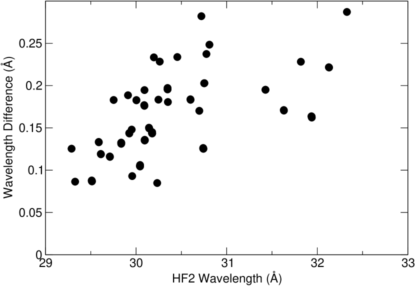
Figure 3: Wavelength differences between MCDF (Chen & Crasemann, 1987) and HF2 for N IV. An average difference of $155\pm 45$ mÅ is observed.

Narrow absorption K$\alpha$ and K$\beta$ lines of N VI have been identified in the warm absorber of the MR 2251-178 quasar, which point to a complex velocity field with an outflow of ionized material (Ramírez et al., 2008). K-shell absorption by Li-like N V, which has prominent UV lines, or by lower charge states at wavelengths $\lambda>29$ Å  is difficult to detect due to the reduced sensitivity of current X-ray instruments towards these longer wavelengths. Notable exceptions include : K$\alpha$ absorption by N V at 29.42 Å has been reported by Steenbrugge et al. (2005) in the outflow of NGC 5548; and N absorption by a white dwarf outflow has been observed following the outburst of nova V4743 Sagittarii (Ness et al., 2003). In the latter case, only the H- and He-lines are discussed, but lower charge states of N are clearly seen in the spectrum longward of 29 Å (see Fig. 3b in Ness et al., 2003).

The current proliferation of X-ray spectra with high signal-to-noise ratio in astronomical archives makes the computation of nitrogen K-shell photoabsorption particularly timely. This is also an additional and important step in the ongoing effort to compute reliable atomic data by García et al. (2005); Palmeri et al. (2008a, b); Witthoeft et al. (2009) for K-line analysis within the context of the xstar spectral modeling code (Kallman & Bautista, 2001). Available spectroscopic data for K-vacancy levels of the N isonuclear sequence are notably scarce, mainly limited to N V and N VI for which a few levels are listed in the NIST database (Ralchenko et al., 2008) and four measured wavelengths have been reported by Beiersdorfer et al. (1999). This shortage of reliable measurements precludes empirical corrections to calculated level energies. On the other hand, several relativistic methods have been previously used to generate atomic data for nitrogen K-vacancy states: the saddle-point complex-rotation method (Davis & Chung, 1989; Chung, 1990; Shiu et al., 2001; Lin et al., 2001, 2002; Zhang et al., 2005); the Raleigh–Ritz variational method (Hsu et al., 1991; Yang & Chung, 1995; Wang & Gou, 2006); and multiconfiguration Dirac–Fock (MCDF) approaches such as those by Hata & Grant (1983); Hardis et al. (1984); Chen (1986); Chen & Crasemann (1987, 1988); Chen et al. (1997). Photoabsorption cross sections in the near K-edge region of N ions have been obtained by Hartree–Slater central-field computations (Reilman & Manson, 1979), where the resonance structure due to quasibound states as well as configuration correlations are neglected. The net effect of the resonance structure is to fill in the photoionization cross section below the inner-shell threshold altering the shape of the K edge.

In this paper we report on calculations of energy level structure and bound-bound and bound-free transition probabilities for the K-shell of nitrogen. The outline of the present report is as follows. The numerical methods are briefly described in § 2 while an analysis of the results based on comparisons with previous experimental and theoretical values is carried out in § 3. The two supplementary electronic tables are explained in § 4 while some conclusions are finally discussed in § 5.

2 Numerical methods

The numerical approach used here has been fully described in Bautista et al. (2003). Level energies, wavelengths, $A$-coefficients, and radiative and Auger rates are computed with the codes autostructure (Eissner et al., 1974; Badnell, 1986, 1997) and hfr (Cowan, 1981). For consistency, configuration-interaction (CI) wave functions of the type

$$\Psi=\sum c_{i}\phi_{i}$$ (1)

are calculated with the relativistic Breit–Pauli Hamiltonian

$$H_{\rm bp}=H_{\rm nr}+H_{\rm 1b}+H_{\rm 2b}$$ (2)

where $H_{\rm nr}$ is the usual non-relativistic Hamiltonian. The one-body relativistic operators

$$H_{\rm 1b}=\sum_{n=1}^{N}{f_{n}({\rm mass})+f_{n}({\rm d})+f_{n}({\rm so})}$$ (3)

represent the spin–orbit interaction, $f_{n}({\rm so})$, the non-fine-structure mass variation, $f_{n}({\rm mass})$, and the one-body Darwin correction, $f_{n}({\rm d})$. The two-body Breit operators are given by

$$H_{\rm 2b}=\sum_{n<m}g_{nm}({\rm so})+g_{nm}({\rm ss})+g_{nm}({\rm css})+g_{nm}({\rm d})+g_{nm}({\rm oo})$$ (4)

where the fine-structure terms are $g_{nm}(so)$ (spin–other-orbit and mutual spin-orbit), $g_{nm}(ss)$ (spin–spin), and the non-fine-structure counterparts $g_{nm}(css)$ (spin–spin contact), $g_{nm}(d)$ (two-body Darwin), and $g_{nm}(oo)$ (orbit–orbit). It must be pointed out that hfr neglects contributions from the two-body term $H_{\rm 2b}$ of Equation (4).

In hfr, core-relaxation effects (CRE) are always taken into account since each electron configuration is represented with its own set of non-orthogonal orbitals optimized by minimizing the average configuration energy. In autostructure, on the other hand, configurations may be represented with either orthogonal or non-orthogonal orbitals which then enables estimates of the importance these effects. In the present calculation five approximations are considered in order to study the effects of electron correlation, i.e. configuration interaction (CI) and CRE, and thus to estimate data accuracy.

Approximation AS1

Atomic data are computed with autostructure including CI from only the $n=2$ complex. CRE are neglected.

Approximation AS2

Atomic data are computed with autostructure including both $n=2$ CI and CRE.

Approximation AS3

Atomic data are computed with autostructure including CI from both the $n=2$ and $n=3$ complexes. CRE are neglected.

Approximation HF1

Atomic data are computed with hfr including CI only from the $n=2$ complex.

Approximation HF2

Atomic data are computed with hfr including CI from both the $n=2$ and $n=3$ complexes.

Photoabsorption cross sections are obtained with the codes Breit-Pauli R-Matrix bprm (Berrington et al., 1987; Seaton, 1987) and hullac (Bar-Shalom et al., 2001). In bprm, wave functions for states of an $N$-electron target and a colliding electron with total angular momentum and parity $J\pi$ are expanded in terms of the target eigenfunctions

$$\Psi^{J\pi}={\cal A}\sum_{i}\chi_{i}{F_{i}(r)\over r}+\sum_{j}c_{j}\Phi_{j}\ .$$ (5)

The $\chi_{i}$ functions are vector coupled products of the target eigenfunctions and the angular components of the incident-electron functions; $F_{i}(r)$ are the radial part of the continuum wave functions that describe the motion of the scattered electron; and $\mathcal{A}$ is an antisymmetrization operator. The functions $\Phi_{j}$ are bound-type functions of the total system constructed with target orbitals. The Breit–Pauli relativistic version has been developed by Scott & Burke (1980) and Scott & Taylor (1982), but the inclusion of the two-body terms (see Equation 4) is currently in progress, and thus not included. Auger and radiative damping are taken into account by means of an optical potential (Robicheaux et al., 1995; Gorczyca & Badnell, 1996; Gorczyca & McLaughlin, 2000) where the resonance energy with respect to the threshold acquires an imaginary component. In the present work, the $N$-electron targets are represented with all the fine structure levels within the $n=2$ complex. It is important to mention that the bprm approach does not allow the inclusion of CRE in the photoionization calculations; therefore, both the initial and final states correspond to configurations represented with orthogonal orbitals. Thus, the wave functions for the target states are those produced with approximation AS1.

hullac (Hebrew University Lawrence Livermore Atomic Code, Bar-Shalom et al., 2001) is a multiconfiguration, relativistic computing package that is based on the relativistic version of the parametric potential method by Klapisch et al. (1977), and employs a factorization-interpolation method within the framework of the distorted wave approximation (Bar-Shalom et al., 1988). It includes the Breit interaction for relativistic configuration averages and can take into account part of the correlation effects by allowing different potentials for each group of configurations. Its newest version (Klapisch & Busquet, 2009), which is used here, incorporates a number of improvements such as important corrections to the photoionization subroutines. For the present work we calculated only transition energies and direct photoionization cross sections, but hullac can also efficiently compute photo-autoionization resonances by means of the isolated resonance approximation (Oreg et al., 1991), which are subsequently superimposed on the continuum photoionization cross section. Moreover, attempts have been made to adapt hullac to calculate the quantum interference of resonances with the continuum that leads to Fano-type asymmetric profiles (Behar et al., 2000, 2004). However, these calculations with hullac are beyond the scope of the present paper.

3 Energy levels

Energies have been computed for both valence and K-vacancy levels in the five approximations delineated in Section 2 and with hullac. A comparison of approximations AS1 with AS2 provides an estimate of CRE while those of AS1 with AS3 and HF1 with HF2 give measures of out-of-complex CI. Also, level energy accuracy can be bound with a comparison of AS2 and HF1, that is, from two physically comparable approximations but calculated with two independent numerical codes.

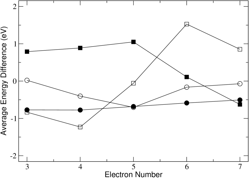
Figure 1: Average level energy differences with respect to approximation AS1 for ions of the nitrogen isonuclear sequence with electron number $3\leq N\leq 7$. Filled circles: valence level energies computed with AS2. Open circles: valence level energies computed with AS3. Filled squares: K-vacancy level energies computed with AS2. Open squares: K-vacancy level energies computed with AS3.

In Figure 1, average energy differences for AS1 vs. AS2 and AS1 vs. AS3 are plotted for each ionic species, $3\leq N\leq 7$. It may be seen that while core relaxation effects lowers the valence-level energies by around 0.5–0.8 eV, it raises by a similar amount those for the K-vacancy levels in species with electron number $3\leq N\leq 5$; as a consequence, transition wavelengths for these ions are expected to be shorter due to this effect. Although $n=3$ CI also causes a lowering (less than 0.7 eV) of the valence level energies (see Figure 1), the impact on the K-vacancy level energies is more pronounced (as large as 1.5 eV): it mainly lowers levels for species with $N<5$ and raises those for $N>5$. The latter result is mostly due to K-vacancy levels from the $n=2$ and $n=3$ complexes intermixing in the lowly ionized members.

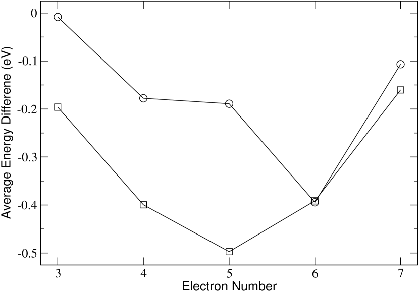
Figure 2: Average level energy differences with respect to approximation HF1 for ions of the nitrogen isonuclear sequence with electron number $3\leq N\leq 7$. Open circles: valence level energies computed with HF2. Open squares: K-vacancy level energies computed with HF2.

Figure 2 shows the corresponding quantities for HF1 and HF2. As shown in Figure 2, the effect of CI on the energies computed with hfr is somewhat different as they are decreased (less than 0.5 eV) for both valence and K-vacancy levels, the minimum occurring in ions with $N=5$ and $N=6$. Level energy differences between the AS2 and HF1 data sets are within 0.5 eV which is a reliable accuracy ranking of the present level energies.

Computed level energies are compared with the few spectroscopic measurements available ($2\leq N\leq 3$) in Table 1. It may be seen that CRE in autostructure (approximation AS2) in general reduce differences with experiment. Furthermore, hfr and hullac seem to provide better energies than autostructure; differences of hfr (hullac) with experiment not being larger than 1.53 eV (1.19 eV). In the He-like system, hullac is particularly accurate for triplet states and less so for singlet states. The accurate approximation of HF2 is compared with previously computed term energies in Table 2. Although we would not quote present term energies with the same number of significant figures as previous results, HF2 values are consistently lower.

Fine-structure level splittings in HF2 can be problematic as shown in Table 3. It may be seen that HF2 gives a value in good accord (1%) with beam-foil measurements for the $\Delta E(^{5}{\rm P}_{2},^{5}{\rm P}_{1})$ splitting of the ${\rm 1s2s2p^{2}\ {}^{5}P}$ K-vacancy term of N iv but an intolerably discrepant one (factor of 2) for $\Delta E(^{5}{\rm P}_{3},^{5}{\rm P}_{2})$. On the other hand, both AS2 splittings are in reasonable agreement (10%) with experiment and with results obtained with the relativistic Raleigh–Ritz variational method (Yang & Chung, 1995; Wang & Gou, 2006) and MCDF (Hata & Grant, 1983; Hardis et al., 1984). This problem has been shown by Hata & Grant (1983) to be due to the neglect of the Breit interaction which is the case in HF2.

The most stringent accuracy requirements for the energies come from the capabilities of the astronomical instruments which can observe these transitions. Current instruments, the Chandra and XMM-Newton gratings, have a resolving power which is nominally $\varepsilon/\Delta\varepsilon\leq$ 1000, which imposes a resolution of $0.4-0.5$ eV in the energy region of the nitrogen K lines ($400-500$ eV), essentially the same accuracy we have achieved in the present calculations. However, in spectra with good statistical signal-to-noise it is possible to determine line centroids to a factor $\sim$3 more accurately than this. Future instruments, principally the grating instruments considered for the International X-ray Observatory (IXO), may also have resolving power as high as 3000. Knowledge of transition wavelengths and energy levels with this precision is needed for truly unambiguous identification of observed features and comparison with models. Clearly, precise laboratory measurements are irreplaceable requisites in the theoretical fine-tuning of these calculations in order to reduce the current uncertainties.

4 Wavelengths

The accuracy of computed wavelengths must be determined without a comparison with measurements due to the scarcity of the latter. CRE and $n=3$ CI in autostructure impact wavelengths in an opposite manner to that displayed for the K-vacancy levels in Figure 1. Specifically, core relaxation on average shortens wavelengths by as much as 150 mÅ in ions with $2\leq N\leq 5$ while the effect is less pronounced on the higher members. CI increases wavelengths by $\sim$50 mÅ for $N\leq 4$ and decreases them by as much as 150 mÅ for $N\geq 5$. CI in hfr in general increases wavelengths with a maximum of 25 mÅ at $N=5$.

Wavelengths computed with AS2 are on average $7\pm 21$ mÅ greater than HF1. This finding can be further appreciated in a comparison with the few available measured wavelengths (see Table 4) where computed values are always greater. HF1 differences with experiment are the smallest (less than 37 mÅ) while CRE in autostructure (AS2) also reduces discrepancies.

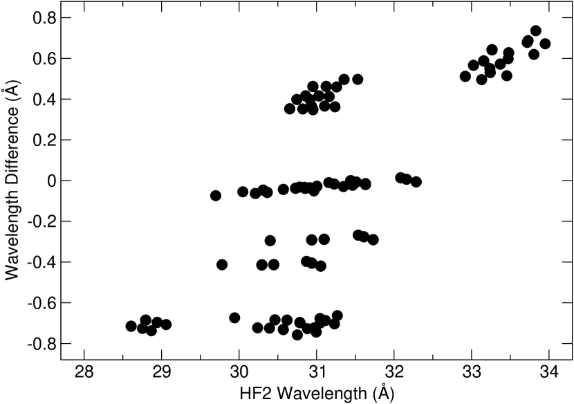
Figure 4: Wavelength differences between MCDF (Chen et al., 1997) and HF2 for N II. Differences as large as 800 mÅ are observed.

Wavelengths for K transitions in nitrogen ions have been previously computed with the MCDF method by Chen (1986); Chen & Crasemann (1987, 1988); Chen et al. (1997). While reasonable agreement is found with HF2 for species with $N=3$ (average difference of $13\pm 25$ mÅ) and $N=5$ (average difference of $-4\pm 33$ mÅ), puzzling discrepancies are found for those with $N=4$ and $N=6$. As shown in Figure 3, the MCDF wavelengths of Chen & Crasemann (1987) show the large average difference with respect to HF2 of $155\pm 45$ mÅ; i.e., on average, they are significantly longer. The inconsistent situation in the C-like ion is somewhat different (see Figure 4) where the average difference with HF2 is now $-45\pm 449$ mÅ showing a very wide and clustered scatter with questionable deviations as large as 800 mÅ. These comparisons lead us to conclude that the wavelengths computed with HF2, our best approximation, are accurate to better than 100 mÅ.

5 $A$-coefficients

By comparing $A$-coefficients computed with approximations AS1 and AS2, CRE on the K radiative decay process may be estimated. Discarding transitions subject to cancellation which always display large differences, it is found that, for $\log A\geq 10$, CRE generally causes differences not greater than 20%. However, larger discrepancies (54%) are found for transitions undergoing multiple electron jumps such as those tabulated in Table 5. $A$-coefficients for these peculiar transitions computed with HF1, which should be comparable to AS2, are also included in Table 5 finding good agreement (within 15%); in fact, differences between $A$-coefficients computed with approximations AS2 and HF1 are in general within 22%. Furthermore, CI from the $n=3$ complex tends to decrease $A$-coefficients with $\log A\geq 10$, AS3 being on average 16% lower than AS1 and HF2 6% lower than HF1.

MCDF $A$-coefficients by Chen (1986); Chen & Crasemann (1987, 1988); Chen et al. (1997) agree with HF2 to around 25% except for $N=6$ where they are found to be, on average, higher by a factor of 4 (see Figure 5). This outcome certainly questions the accuracy of the MCDF $A$-coefficients by Chen et al. (1997) for C-like nitrogen. We find that for $\log A\geq 10$ present $A$-coefficients are accurate to within 20% for transitions not affected by cancellation.

6 Radiative widths

A comparison of AS1 and AS2 radiative widths for the K-vacancy levels indicates that CRE are mainly noticeable in the highly ionized species, namely those with $N\leq 4$, where on average the radiative widths are increased by around 10%. On the other hand, the inclusion of levels from the $n=3$ complex in the CI expansion (AS3) leads to slightly reduced radiative widths (less than 7%) with respect to AS1 for the lowly ionized members ($N\geq 5$). Larger reductions ($\sim$20%) are also observed for the lowly ionized species between HF2 (which contains CI from the $n=3$ complex) and HF1 (which contains CI only from the $n=2$ complex).

A remarkable exception is the radiative width of the ${\rm 1s2s^{2}2p^{3}\ {}^{5}S^{o}_{2}}$ level in the C-like ion. For this level, AS2 gives $A_{j}=\sum_{i}A_{ji}=7.09\times 10^{6}$ s^-1 in good agreement with HF1 ($7.65\times 10^{6}$ s^-1); however, the AS3 and HF2 radiative widths are respectively $A_{j}=5.31\times 10^{8}$ s^-1 and $A_{j}=3.77\times 10^{9}$ s^-1, i.e. around two orders of magnitude larger. The reason for this huge increase when levels from $n=3$ complex are included in the CI expansion may be appreciated in Table 6. Within the $n=2$ complex, the ${\rm 1s2s^{2}2p^{3}\ {}^{5}S^{o}_{2}}$ decays radiatively to the ${\rm 1s^{2}2s^{2}2p^{2}\ {}^{3}P_{j}}$ ground levels via two spin-forbidden K$\alpha$ transitions which have small $A$-coefficients ($\lesssim 10^{7}$ s^-1). When the $n=3$ complex is taken into account, $3\rightarrow 2$ spin-allowed channels appear which exhibit considerably larger $A$-coefficients that add up to the quoted enhancement. The observed discrepancy between AS3 and HF2 (a factor of 7) are due to severe cancellation in the $\Delta n\neq 0$ transitions.

Radiative widths computed for ions with electron number $3\leq N\leq 6$ with the MCDF method (Chen, 1986; Chen & Crasemann, 1987, 1988; Chen et al., 1997) agree with HF2 to around 20% except for the C-like species where MCDF is a factor of 4.6 higher.

7 Auger widths

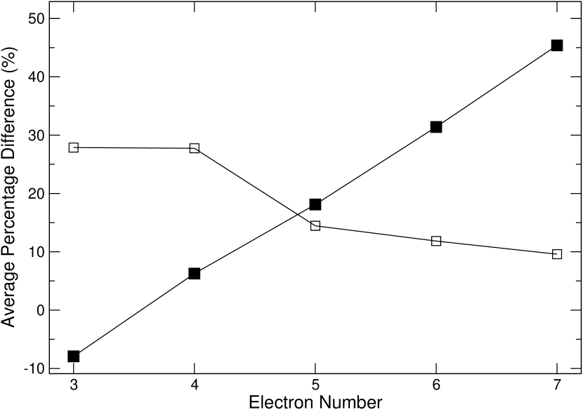
Figure 6: Average percentage difference between Auger widths ($\log A_{\rm a}\geq 12$) computed with the AS2 and AS1 approximations (filled squares) and with AS3 and AS1 (open squares).

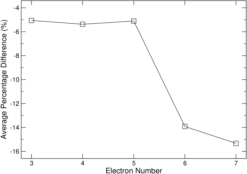
Figure 7: Average percentage difference between Auger widths ($\log A_{\rm a}\geq 12$) computed with the HF2 and HF1.

Auger widths computed with AS2 and HF1 agree to within 20% but are sensitive to both CRE and CI as depicted in Figures 6–7. A comparison of AS1 and AS2 shows that, on average, CRE effects increase Auger widths with $\log A_{\rm a}\geq 12$ linearly as a function of the ion electron number $N$. In autostructure CI also increases Auger widths, particularly for highly ionized species (around 28% for ions with $3\leq N\leq 4$) while in hfr Auger widths are decreased (up to 15% for the lowly ionized members). We believe these contrasting outcomes are due to the way orbitals have been optimized in autostructure.

Excluding the C-like ion, MCDF Auger widths by Chen (1986); Chen & Crasemann (1987, 1988); Chen et al. (1997) with $\log A_{\rm a}\geq 12$ in general agree with HF2 to around 20%. Larger discrepancies are encountered for a handful of K-vacancy levels listed in Table 7 which are mainly caused by level admixture. It may be seen therein that Auger widths computed with our different approximations also display a wide scatter thus supporting this diagnostic. For the C-like ion, the MCDF Auger widths are, on average, a factor of 3 higher than HF2 and thus believed to be of poor quality.

In Table 8, Auger widths for the 1s2s2p levels of N V computed with the Breit–Pauli saddle-point complex-rotation method (Davis & Chung, 1989) are compared with AS2, HF2, and the MCDF values of Chen (1986). The agreement with AS2 is within 15% while very large differences are found for the HF2 ${\rm{}^{4}P^{o}_{j}}$ levels which are most surely due to the neglect of the two-body Breit interaction in hfr. The accord with MCDF is around 25% except for the ${\rm 1s2s2p\ ^{2}P^{o}}$ term where a discrepancy of a factor of 2 is encountered. The latter is difficult to explain.

Auger widths for K-vacancy terms in N IV computed with the Breit–Pauli saddle-point complex-rotation method (Lin et al., 2001, 2002; Zhang et al., 2005) are compared with AS2, HF2, and MCDF (Chen & Crasemann, 1987) in Table 9. The level of agreement with AS2 and HF2 is around 20% except for the values quoted by Zhang et al. (2005) for the ${\rm 1s2p^{3}\ {}^{3}P^{o}}$ and ${\rm{}^{3}D^{o}}$ terms which are discrepant by about 50%, in contrast with the MCDF Auger widths for these two terms which agree with AS2 and HF2 to within 10%. The rest of the MCDF Auger widths are in good agreement except for the ${\rm 1s2s2p^{2}\ {}^{3}P}$ term which has already been singled out in Table 7 as being sensitive to level mixing.

8 Photoabsorption cross sections

In Figure 8, we show the high-energy photoabsorption cross sections of N I – N V computed with the bprm package. Intermediate coupling has been used by implementing the AS1 approximation to describe the target wave functions. In order to resolve accurately the K-threshold region, radiative and Auger damping are taken into account as described by Gorczyca & McLaughlin (2000) using the Auger widths calculated with the HF2 approximation. For comparison, we have included the photoionization cross sections obtained with the hullac code and those by Reilman & Manson (1979), the latter calculated in a central-field potential. This comparison shows that the K-threshold energies of bprm and hullac are in very good accord (within 1 eV) and the background cross sections to within $\sim 10\%$. Note that for the sake of comparison, we have used hullac only to compute the direct bound-free photoionization cross section and not the resonances. Background cross sections by Reilman & Manson (1979) are in excellent agreement with bprm for all ions, but K-edge positions and structures are clearly discrepant. The present bprm calculations result in smeared K edges due to the dominance of the Auger spectator (KLL) channels over the participator (KL$n$) channels. This overall behavior is similar to that reported in previous calculations (Kallman et al., 2004; Witthoeft et al., 2009), and in particular to that displayed by the corresponding oxygen ions (see Figure 5 in García et al., 2005).

9 Machine-readable tables

We include two machine readable tables. For nitrogen ions with electron occupancy $N=1-7$ and for both valence and Auger levels, Table 10 tabulates the spin multiplicity, total orbital angular momentum and total angular momentum quantum numbers, configuration assignment, energy, and radiative and Auger widths. Fields not applicable or not computed are labeled with the identifier “$-9.99$E$+2$”. For K transitions, Table 11 tabulates the wavelength, $A$-coefficient, and $gf$-value. The printed stub versions list the corresponding data only for the Li-like ion ($N=3$). The photoionization curves may be requested from the corresponding author.

10 Discussion and conclusions

Detailed calculations have been carried out on the atomic properties of K-vacancy states in ions of the nitrogen isonuclear sequence. Data sets containing energy levels, wavelengths, $A$-coefficients and radiative and Auger widths for K-vacancy levels have been computed with the atomic structure codes hfr and autostructure. High-energy photoionization and photoabsorption cross sections for members with electron occupancies $N\geq 3$ have been calculated with the bprm and hullac codes.

Our best approximation (HF2) takes into account both core-relaxation effects and configuration interaction from the $n=3$ complex. By comparing results from different approximations with previous theoretical work and the few spectroscopic measurements available, we conclude that level energies and wavelengths for all the nitrogen ions considered in the present calculations can be quoted to be accurate to within 0.5 eV and 100 mÅ, respectively. The accuracy of $A$-coefficients and radiative and Auger widths is estimated at approximately 20% for transitions neither affected by cancelation nor strong level admixture. Outstanding discrepancies are found with some MCDF data, in particular wavelengths and $A$-coefficients for the C-like ion which are believed to be due to numerical error by Chen et al. (1997).

We have also presented detailed photoabsorption cross sections of nitrogen ions in the near K-threshold region. Due to the lack of previous experimental and theoretical results, we have also performed simpler calculations using the hullac code in order to check for consistency and to estimate accuracy. Comparison of bprm and hullac indicates that present K-threshold energies are accurate to within 1 eV. However, background cross sections are in better agreement with those computed by Reilman & Manson (1979) in a central-field potential for all ions except the Li-like system. These photoabsorption cross sections and their structures are similar to those displayed by ions in the same isoelectronic sequence (Witthoeft et al., 2009), especially to the corresponding oxygen ions (García et al., 2005).

The present atomic data sets are available on request and will be incorporated in the xstar modeling code in order to generate improved opacities in the nitrogen K-edge region, which will lead to useful astrophysical diagnostics such as those mentioned in § 1.

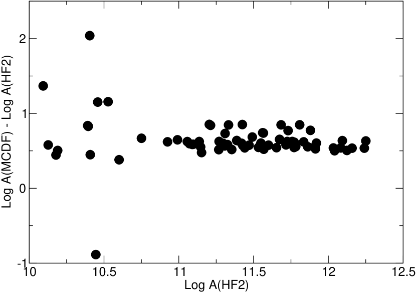
Figure 5: $A$-coefficient differences (s^-1) between MCDF (Chen et al., 1997) and HF2 for N II. It is found that MCDF is on average higher by a factor of 4.

Figure 8: High-energy photoabsorption cross sections for nitrogen ions in the K-edge region. Solid curve: bprm. Dotted curve: hullac. Dashed curve: Reilman & Manson (1979).

Table 1: Measured and computed $K$-vacancy level energies (eV)

$N$	Level	$E$	$E({\rm Th})-E({\rm Expt})$
		Expt	AS1	AS2	AS3	HF1	HF2	hullac
2	${\rm 1s2s\ ^{3}S_{1}}$	419.80	$-$1.76	$-$1.34	$-$2.35	$-$0.59		0.01
2	${\rm 1s2p\ ^{3}P^{o}_{0}}$	426.30	$-$1.85	$-$0.93	$-$2.36	$-$0.56		0.09
2	${\rm 1s2p\ ^{3}P^{o}_{1}}$	426.30	$-$1.85	$-$0.93	$-$2.36	$-$0.54		0.11
2	${\rm 1s2p\ ^{3}P^{o}_{2}}$	426.33	$-$1.86	$-$0.94	$-$2.37	$-$0.53		0.13
2	${\rm 1s2s\ ^{1}S_{0}}$	426.42	$-$1.61	$-$0.21	$-$2.15	0.03		0.69
2	${\rm 1s2p\ ^{1}P^{o}_{1}}$	430.70	$-$1.64	$-$0.85	$-$2.24	$-$0.24		0.67
3	${\rm 1s(^{2}S)2s2p(^{3}P^{o})\ ^{4}P^{o}_{5/2}}$	414.61	$-$2.49	$-$1.97	$-$3.64	$-$1.48	$-$1.53	0.42
3	${\rm 1s(^{2}S)2s2p(^{3}P^{o})\ ^{2}P^{o}_{3/2}}$	421.52	$-$1.72	$-$0.80	$-$2.18	$-$0.51	$-$0.62	0.83
3	${\rm 1s(^{2}S)2p^{2}(^{3}P)\ ^{4}P_{5/2}}$	425.70	$-$2.54	$-$1.64	$-$3.37	$-$1.31	$-$1.33	1.19

Note. — Experimental level energies (relative to the ion ground state) from the NIST database (Ralchenko et al., 2008).

Table 2: Computed total energies (au) for $K$-vacancy terms

$N$	Term	HF2	Other theory
3	${\rm 1s2s2p\ ^{4}P^{o}}$	$-$33.240	$-$33.192008, $-$33.192204
3	${\rm 1s(^{2}S)2s2p(^{3}P^{o})\ ^{2}P^{o}}$	$-$32.952	$-$32.919222
3	${\rm 1s(^{2}S)2s2p(^{1}P^{o})\ ^{2}P^{o}}$	$-$32.777	$-$32.768550
4	${\rm 1s2s^{2}2p\ ^{3}P^{o}}$	$-$36.219	$-$36.171232, $-$36.173064
4	${\rm 1s2s2p^{2}\ {}^{3}S}$	$-$35.646	$-$35.615357
4	${\rm 1s2s2p^{2}\ {}^{3}P}$	$-$35.842	$-$35.788866
4	${\rm 1s2s2p^{2}\ {}^{3}P}$	$-$35.542	$-$35.536868
4	${\rm 1s2s2p^{2}\ {}^{3}D}$	$-$35.815	$-$35.785042
4	${\rm 1s2s^{2}2p\ ^{1}P^{o}}$	$-$36.081	$-$36.036967
4	${\rm 1s2p^{3}\ {}^{1}P^{o}}$	$-$35.086	$-$35.082958
4	${\rm 1s2s2p^{2}\ {}^{1}D}$	$-$35.594	$-$35.583448
4	${\rm 1s2s2p^{2}\ {}^{1}P}$	$-$35.445	$-$35.435017
4	${\rm 1s2s2p^{2}\ {}^{1}S}$	$-$35.425	$-$35.415017
4	${\rm 1s2s2p^{2}\ {}^{5}P}$	$-$36.160	$-$36.0934586, $-$36.0934407
4	${\rm 1s2p^{3}\ {}^{5}S^{o}}$	$-$35.596	$-$35.5414665, $-$35.5413248
4	${\rm 1s2p^{3}\ {}^{3}P^{o}}$	$-$35.214	$-$35.204065
4	${\rm 1s2p^{3}\ {}^{3}D^{o}}$	$-$35.387	$-$35.366601

Table 3: Level splittings (cm^-1) for the ${\rm 1s2s2p^{2}\ {}^{5}P}$ K-vacancy term of N IV

Level splitting	Expt	HF2	AS2	Other theory
$\Delta E(^{5}{\rm P}_{2},^{5}{\rm P}_{1})$	127$\pm$ 1	126	119	127.07, 126.9, 129.19, 128.94
$\Delta E(^{5}{\rm P}_{3},^{5}{\rm P}_{2})$	79.5$\pm$ 0.8	188	70	78.49, 78.45, 86.72, 86.58

Table 4: Experimental and theoretical wavelengths (Å) for nitrogen ions

$N$	Lower level	Upper level	$\lambda$(Expt)	$\lambda({\rm Th})-\lambda({\rm Expt})$
				HF1	AS1	AS2	AS3	hullac
2	${\rm 1s^{2}\ {}^{1}S_{0}}$	${\rm 1s2s\ ^{3}S_{1}}$	$29.5321(26)$		0.1266	0.0971	0.1683	0.0012
2	${\rm 1s^{2}\ {}^{1}S_{0}}$	${\rm 1s2p\ ^{3}P^{o}_{1}}$	$29.0835(26)$	0.0374	0.1274	0.0642	0.1627	–0.0074
2	${\rm 1s^{2}\ {}^{1}S_{0}}$	${\rm 1s2p\ ^{1}P^{o}_{1}}$	$28.7861(22)$	0.0167	0.1108	0.0576	0.1515	–0.0444
3	${\rm 1s^{2}2s\ ^{2}S_{1/2}}$	${\rm 1s2s2p\ ^{2}P^{o}_{3/2}}$	$29.4135(37)$	0.0353	0.1208	0.0560	0.1550	–0.0573

Table 5: Core relaxation effects on K radiative decay

$N$	$j$	$i$	$A_{ji}$ (s${}^{-1})$
			AS1	AS2	HF1
3	${\rm 1s2s^{2}\ {}^{2}S_{1/2}}$	${\rm 1s^{2}2p\ ^{2}P^{o}_{1/2}}$	3.85E$+$10	5.36E$+$10	4.63E$+$10
3	${\rm 1s2s^{2}\ {}^{2}S_{1/2}}$	${\rm 1s^{2}2p\ ^{2}P^{o}_{3/2}}$	7.62E$+$10	1.06E$+$11	9.18E$+$10
4	${\rm 1s2s^{2}2p\ ^{1}P^{o}_{1}}$	${\rm 1s^{2}2p^{2}\ {}^{1}D_{2}}$	9.72E$+$10	1.36E$+$11	1.24E$+$11
5	${\rm 1s2s^{2}2p^{2}\ {}^{2}P_{1/2}}$	${\rm 1s^{2}2p^{3}\ {}^{2}P^{o}_{1/2}}$	1.17E$+$10	1.80E$+$10	1.78E$+$10
5	${\rm 1s2s^{2}2p^{2}\ {}^{2}P_{3/2}}$	${\rm 1s^{2}2p^{3}\ {}^{2}P^{o}_{3/2}}$	1.54E$+$10	2.36E$+$10	2.32E$+$10

Table 6: Radiative decay routes of ${\rm 1s2s^{2}2p^{3}\ {}^{5}S^{o}_{2}}$ in N II

$j$	$i$	$A_{ji}$ (s${}^{-1})$
		AS3	HF2
${\rm 1s2s^{2}2p^{3}\ {}^{5}S^{o}_{2}}$	${\rm 1s^{2}2s^{2}2p^{2}\ {}^{3}P_{1}}$	2.04E$+$6	8.57E$+$6
	${\rm 1s^{2}2s^{2}2p^{2}\ {}^{3}P_{2}}$	2.97E$+$6	2.53E$+$7
	${\rm 1s^{2}2s2p^{2}3d\ ^{5}P_{1}}$	5.07E$+$7	3.43E$+$8
	${\rm 1s^{2}2s2p^{2}3d\ ^{5}P_{2}}$	8.36E$+$7	5.70E$+$8
	${\rm 1s^{2}2s2p^{2}3d\ ^{5}P_{3}}$	1.17E$+$8	7.97E$+$8
	${\rm 1s^{2}2p^{3}3p\ ^{5}P_{1}}$	7.85E$+$7	6.99E$+$8
	${\rm 1s^{2}2p^{3}3p\ ^{5}P_{2}}$	1.31E$+$7	1.16E$+$9
	${\rm 1s^{2}2p^{3}3p\ ^{5}P_{3}}$	1.83E$+$8	1.63E$+$8
$\sum_{i}A_{ji}$		5.31E$+$8	3.77E$+$9

Table 7: Discrepant Auger rates (s^-1)

$N$	Level	AS1	AS2	AS3	HF1	HF2	MCDF
3	${\rm 1s(^{2}S)2s2p(^{3}P^{o})\ ^{2}P^{o}_{1/2}}$	1.51E+13	5.81E+12	2.15E+13	8.61E+12	7.63E+12	1.41E+13
3	${\rm 1s(^{2}S)2s2p(^{3}P^{o})\ ^{2}P^{o}_{3/2}}$	1.43E+13	5.27E+12	2.02E+13	8.29E+12	7.30E+12	1.35E+13
4	${\rm 1s(^{2}S)2s2p^{2}(^{4}P)\ ^{3}P_{0}}$	3.09E+13	1.99E+13	4.41E+13	1.86E+13	1.77E+13	3.73E+13
4	${\rm 1s(^{2}S)2s2p^{2}(^{4}P)\ ^{3}P_{1}}$	3.08E+13	1.98E+13	4.40E+13	1.86E+13	1.76E+13	3.68E+13
4	${\rm 1s(^{2}S)2s2p^{2}(^{4}P)\ ^{3}P_{2}}$	3.04E+13	1.95E+13	4.36E+13	1.85E+13	1.75E+13	3.55E+13
4	${\rm 1s(^{2}S)2s2p^{2}(^{2}P)\ ^{1}P_{1}}$	2.26E+13	2.88E+13	2.62E+13	2.46E+13	2.34E+13	1.43E+14
4	${\rm 1s(^{2}S)2s2p^{2}(^{2}S)\ ^{1}S_{0}}$	1.34E+14	1.33E+14	1.77E+14	1.28E+14	1.19E+14	1.77E+13
5	${\rm 1s(^{2}S)2s2p^{3}(^{5}S^{o})\ ^{4}S^{o}_{3/2}}$	3.90E+13	2.98E+13	4.10E+13	2.54E+13	2.48E+13	3.89E+13
5	${\rm 1s(^{2}S)2s2p^{3}(^{3}S^{o})\ ^{2}S^{o}_{1/2}}$	2.34E+13	3.09E+13	2.88E+13	5.30E+13	1.31E+14	3.49E+13
5	${\rm 1s(^{2}S)2s2p^{3}(^{1}P^{o})\ ^{2}P^{o}_{1/2}}$	1.37E+14	1.67E+14	1.56E+14	1.27E+14	3.48E+13	1.52E+14

Table 8: Auger energy widths (au) for 1s2s2p levels in N V

Level	AS2	HF2	Other theory
${\rm 1s(^{2}S)2s2p(^{3}P^{o})\ ^{4}P^{o}_{1/2}}$	1.46E$-$08	3.48E$-10$	1.50E$-08$, 1.532E$-$08
${\rm 1s(^{2}S)2s2p(^{3}P^{o})\ ^{4}P^{o}_{3/2}}$	4.53E$-$09	8.83E$-10$	4.98E$-09$, 3.952E$-$09
${\rm 1s(^{2}S)2s2p(^{3}P^{o})\ ^{4}P^{o}_{5/2}}$	4.26E$-$10		4.587E$-$10
${\rm 1s(^{2}S)2s2p(^{3}P^{o})\ ^{2}P^{o}}$	1.32E$-$04	1.79E$-04$	3.31E$-$04, 1.54E$-$04
${\rm 1s(^{2}S)2s2p(^{1}P^{o})\ ^{2}P^{o}}$	1.68E$-$03	1.47E$-03$	1.14E$-$03, 1.53E$-$03

Table 9: Auger widths (meV) for $K$-vacancy terms in N IV

Term	AS2	HF2	Other theory
${\rm 1s2s^{2}2p\ ^{3}P^{o}}$	84.1	71.8	77.4, 79.0
${\rm 1s(^{2}S)2s2p^{2}(^{4}P)\ ^{3}P}$	12.9	11.6	23.8, 10.8
${\rm 1s(^{2}S)2s2p^{2}(^{2}D)\ ^{3}D}$	66.9	62.6	53.4, 57.7
${\rm 1s(^{2}S)2s2p^{2}(^{2}S)\ ^{3}S}$	31.2	29.7	26.7, 28.6
${\rm 1s(^{2}S)2s2p^{2}(^{2}P)\ ^{3}P}$	66.4	55.5	58.5, 55.0
${\rm 1s2s^{2}2p\ ^{1}P^{o}}$	55.2	48.3	53.8, 58
${\rm 1s2p^{3}\ {}^{1}P^{o}}$	44.9	47.0	43.8, 43
${\rm 1s2p^{3}\ {}^{3}D^{o}}$	80.7	80.3	75.0, 53.87
${\rm 1s2p^{3}\ {}^{3}P^{o}}$	47.4	47.5	45.5, 34.16

Table 10: Valence and Auger levels for nitrogen ions

$N$	$i$	$2S+1$	$L$	$2J$	Configuration	Energy	$A$r	$A$a
						eV	s-1	s-1
3	1	2	0	1	1s22s 2S1/2	0.0000	$-$9.99E+02	$-$9.99E+02
3	2	2	1	1	1s22p 2Po1/2	9.9459	3.32E+08	$-$9.99E+02
3	3	2	1	3	1s22p 2Po3/2	9.9774	3.35E+08	$-$9.99E+02
3	4	2	0	1	1s2s2 2S1/2	410.1562	1.22E+11	9.79E+13
3	5	4	1	1	1s(2S)2s2p(3Po) 4Po1/2	413.0288	5.05E+06	1.44E+07
3	6	4	1	3	1s(2S)2s2p(3Po) 4Po3/2	413.0471	1.27E+07	3.65E+07
3	7	4	1	5	1s(2S)2s2p(3Po) 4Po5/2	413.0778	0.00E+00	1.76E+07
3	8	2	1	1	1s(2S)2s2p(3Po) 2Po1/2	420.8755	1.65E+12	7.63E+12
3	9	2	1	3	1s(2S)2s2p(3Po) 2Po3/2	420.8968	1.65E+12	7.30E+12
3	10	4	1	1	1s(2S)2p2(3P) 4P1/2	424.3267	7.99E+08	5.54E+06
3	11	4	1	3	1s(2S)2p2(3P) 4P3/2	424.3446	8.06E+08	4.65E+08
3	12	4	1	5	1s(2S)2p2(3P) 4P5/2	424.3741	8.15E+08	2.85E+09
3	13	2	1	1	1s(2S)2s2p(1Po) 2Po1/2	425.6391	1.63E+11	6.06E+13
3	14	2	1	3	1s(2S)2s2p(1Po) 2Po3/2	425.6545	1.55E+11	6.10E+13
3	15	2	2	3	1s(2S)2p2(1D) 2D3/2	429.2436	8.33E+11	1.07E+14
3	16	2	2	5	1s(2S)2p2(1D) 2D5/2	429.2442	8.32E+11	1.07E+14
3	17	2	1	1	1s(2S)2p2(3P) 2P1/2	430.3236	2.68E+12	1.20E+08
3	18	2	1	3	1s(2S)2p2(3P) 2P3/2	430.3597	2.68E+12	4.50E+10
3	19	2	0	1	1s(2S)2p2(1S) 2S1/2	437.1874	7.86E+11	1.60E+13

Note. — A complete machine-readable version of this table may be accessed on-line.

Table 11: Radiative K-transition data nitrogen ions

$N$	$j$	$i$	Wavelength	$A$-coefficient	$gf$-value
			0.1 nm	s-1
3	4	2	30.9798	4.08E$+$10	1.17E$-$02
3	4	3	30.9822	8.08E$+$10	2.33E$-$02
3	5	1	30.0183	5.05E$+$06	1.36E$-$06
3	6	1	30.0170	1.27E$+$07	6.87E$-$06
3	8	1	29.4586	1.65E$+$12	4.29E$-$01
3	9	1	29.4571	1.65E$+$12	8.61E$-$01
3	10	2	29.9203	9.70E$+$06	2.61E$-$06
3	10	3	29.9226	2.36E$+$05	6.34E$-$08
3	11	2	29.9191	7.01E$+$04	3.77E$-$08
3	11	3	29.9213	1.58E$+$07	8.49E$-$06
3	12	3	29.9192	2.14E$+$07	1.72E$-$05
3	13	1	29.1289	1.62E$+$11	4.12E$-$02
3	14	1	29.1279	1.54E$+$11	7.83E$-$02
3	15	2	29.5695	7.16E$+$11	3.76E$-$01
3	15	3	29.5717	1.17E$+$11	6.12E$-$02
3	16	3	29.5717	8.32E$+$11	6.55E$-$01
3	17	2	29.4935	1.79E$+$12	4.68E$-$01
3	17	3	29.4957	8.89E$+$11	2.32E$-$01
3	18	2	29.4910	4.24E$+$11	2.21E$-$01
3	18	3	29.4932	2.26E$+$12	1.18E$+$00
3	19	2	29.0197	2.56E$+$11	6.46E$-$02
3	19	3	29.0218	5.28E$+$11	1.33E$-$01

Note. — A complete machine-readable version of this table may be accessed on-line.

References

- Arav et al. (2007) Arav, N., et al. 2007, ApJ, 658, 829
- Badnell (1986) Badnell, N. R. 1986, J. Phys. B, 19, 3827
- Badnell (1997) —. 1997, J. Phys. B, 30, 1
- Bar-Shalom et al. (1988) Bar-Shalom, A., Klapisch, M., & Oreg, J. 1988, Phys. Rev. A, 38, 1773
- Bar-Shalom et al. (2001) —. 2001, J. Quant. Spectrosc. Radiat. Transfer, 71, 169
- Bautista et al. (2003) Bautista, M. A., Mendoza, C., Kallman, T. R., & Palmeri, P. 2003, A&A, 403, 339
- Behar et al. (2000) Behar, E., Jacobs, V. L., Oreg, J., Bar-Shalom, A., & Haan, S. L. 2000, Phys. Rev. A, 62, 030501
- Behar et al. (2004) —. 2004, Phys. Rev. A, 69, 022704
- Behar & Netzer (2002) Behar, E., & Netzer, H. 2002, ApJ, 570, 165
- Behar et al. (2003) Behar, E., Rasmussen, A. P., Blustin, A. J., Sako, M., Kahn, S. M., Kaastra, J. S., Branduardi-Raymont, G., & Steenbrugge, K. C. 2003, ApJ, 598, 232
- Behar et al. (2001) Behar, E., Sako, M., & Kahn, S. M. 2001, ApJ, 563, 497
- Beiersdorfer et al. (1999) Beiersdorfer, P., López-Urrutia, J. R. C., Springer, P., Utter, S. B., & Wong, K. L. 1999, Rev. Sci. Instrum., 70, 276
- Berrington et al. (1987) Berrington, K. A., Burke, P. G., Butler, K., Seaton, M. J., Storey, P. J., Taylor, K. T., & Yan, Y. 1987, J. Phys. B, 20, 6379
- Berry et al. (1982) Berry, H. G., Brooks, R. L., Cheng, K. T., Hardis, J. E., & Ray, W. 1982, Phys. Scr, 25, 391
- Brinkman et al. (2002) Brinkman, A. C., Kaastra, J. S., van der Meer, R. L. J., Kinkhabwala, A., Behar, E., Kahn, S. M., Paerels, F. B. S., & Sako, M. 2002, A&A, 396, 761
- Chen (1986) Chen, M. H. 1986, At. Data Nucl. Data Tables, 34, 301
- Chen & Crasemann (1987) Chen, M. H., & Crasemann, B. 1987, At. Data Nucl. Data Tables, 37, 419
- Chen & Crasemann (1988) —. 1988, At. Data Nucl. Data Tables, 38, 381
- Chen et al. (1997) Chen, M. H., Reed, K. J., McWilliams, D. M., Guo, D. S., Barlow, L., Lee, M., & Walker, V. 1997, At. Data Nucl. Data Tables, 65, 289
- Chung (1990) Chung, K. T. 1990, Phys. Rev. A, 42, 645
- Cowan (1981) Cowan, R. D. 1981, The Theory of Atomic Structure and Spectra (Berkeley, CA: Univ. California Press)
- Davis & Chung (1989) Davis, B. F., & Chung, K. T. 1989, Phys. Rev. A, 39, 3942
- Eissner et al. (1974) Eissner, W., Jones, M., & Nussbaumer, H. 1974, Comput. Phys. Commun., 8, 270
- Favata et al. (2009) Favata, F., Neiner, C., Testa, P., Hussain, G., & Sanz-Forcada, J. 2009, A&A, 495, 217
- García et al. (2005) García, J., Mendoza, C., Bautista, M. A., Gorczyca, T. W., Kallman, T. R., & Palmeri, P. 2005, ApJS, 158, 68
- Gorczyca & Badnell (1996) Gorczyca, T. W., & Badnell, N. R. 1996, J. Phys. B, 29, L283
- Gorczyca & McLaughlin (2000) Gorczyca, T. W., & McLaughlin, B. M. 2000, J. Phys. B, 33, L859
- Hardis et al. (1984) Hardis, J. E., Berry, H. G., Curtis, L. J., & Livingston, A. E. 1984, Phys. Scr, 30, 189
- Hata & Grant (1983) Hata, J., & Grant, I. P. 1983, J. Phys. B, 16, L125
- Hsu et al. (1991) Hsu, J.-J., Chung, K. T., & Huang, K.-N. 1991, Phys. Rev. A, 44, 5485
- Kaastra et al. (2009) Kaastra, J. S., de Vries, C. P., Costantini, E., & den Herder, J. W. A. 2009, A&A, 497, 291
- Kallman & Bautista (2001) Kallman, T., & Bautista, M. 2001, ApJS, 133, 221
- Kallman et al. (2004) Kallman, T. R., Palmeri, P., Bautista, M. A., Mendoza, C., & Krolik, J. H. 2004, ApJS, 155, 675
- Klapisch & Busquet (2009) Klapisch, M., & Busquet, M. 2009, High Ener. Dens. Phys., 5, 105
- Klapisch et al. (1977) Klapisch, M., Schwob, J. L., Fraenkel, B. S., & Oreg, J. 1977, J. Opt. Soc. Am., 67, 148
- Leutenegger et al. (2003) Leutenegger, M. A., Kahn, S. M., & Ramsay, G. 2003, ApJ, 585, 1015
- Lin et al. (2002) Lin, H., Hsue, C.-S., & Chung, K. T. 2002, Phys. Rev. A, 65, 032706
- Lin et al. (2001) Lin, S.-H., Hsue, C.-S., & Chung, K. T. 2001, Phys. Rev. A, 64, 012709
- Miyata et al. (2008) Miyata, E., Masai, K., & Hughes, J. P. 2008, PASJ, 60, 521
- Ness et al. (2003) Ness, J.-U., et al. 2003, ApJ, 594, L127
- Oreg et al. (1991) Oreg, J., Goldstein, W. H., Klapisch, M., & Bar-Shalom, A. 1991, Phys. Rev. A, 44, 1750
- Palmeri et al. (2008a) Palmeri, P., Quinet, P., Mendoza, C., Bautista, M. A., García, J., & Kallman, T. R. 2008a, ApJS, 177, 408
- Palmeri et al. (2008b) Palmeri, P., Quinet, P., Mendoza, C., Bautista, M. A., García, J., Witthoeft, M. C., & Kallman, T. R. 2008b, ApJS, 179, 542
- Pradhan (2000) Pradhan, A. K. 2000, ApJ, 545, L165
- Ralchenko et al. (2008) Ralchenko, Y., Kramida, A. E., Reader, J., & NIST ADS Team. 2008, NIST Atomic Spectra Database, version 3.1.5 (Gaithersburg: NIST), http://physics.nist.gov/asd3
- Ramírez et al. (2008) Ramírez, J. M., Komossa, S., Burwitz, V., & Mathur, S. 2008, ApJ, 681, 965
- Reilman & Manson (1979) Reilman, R. F., & Manson, S. T. 1979, ApJS, 40, 815
- Robicheaux et al. (1995) Robicheaux, F., Gorczyca, T. W., Pindzola, M. S., & Badnell, N. R. 1995, Phys. Rev. A, 52, 1319
- Sako et al. (2001) Sako, M., et al. 2001, A&A, 365, L168
- Scott & Burke (1980) Scott, N. S., & Burke, P. G. 1980, J. Phys. B, 13, 4299
- Scott & Taylor (1982) Scott, N. S., & Taylor, K. T. 1982, Comput. Phys. Commun., 25, 347
- Seaton (1987) Seaton, M. 1987, J. Phys. B At. Mol. Phys., 20, 6363
- Shiu et al. (2001) Shiu, W. C., Hsue, C.-S., & Chung, K. T. 2001, Phys. Rev. A, 64, 022714
- Steenbrugge et al. (2005) Steenbrugge, K. C., et al. 2005, A&A, 434, 569
- Wang & Gou (2006) Wang, F., & Gou, B. C. 2006, At. Data Nucl. Data Tables, 92, 176
- Witthoeft et al. (2009) Witthoeft, M. C., Bautista, M. A., Mendoza, C., Kallman, T. R., Palmeri, P., & Quinet, P. 2009, ApJS, 182, 127
- Yang & Chung (1995) Yang, H. Y., & Chung, K. T. 1995, Phys. Rev. A, 51, 3621
- Yao et al. (2009) Yao, Y., Schulz, N. S., Gu, M. F., Nowak, M. A., & Canizares, C. R. 2009, ApJ, 696, 1418
- Zhang et al. (2005) Zhang, M., Gou, B. C., & Cui, L. L. 2005, J. Phys. B, 38, 3567