Minimal Curvature Trajectories: Riemannian Geometry Concepts for Model Reduction in Chemical Kinetics

Abstract

In dissipative ordinary differential equation systems different time scales cause anisotropic phase volume contraction along solution trajectories. Model reduction methods exploit this for simplifying chemical kinetics via a time scale separation into fast and slow modes. The aim is to approximate the system dynamics with a dimension-reduced model after eliminating the fast modes by enslaving them to the slow ones via computation of a slow attracting manifold. We present a novel method for computing approximations of such manifolds using trajectory-based optimization. We discuss Riemannian geometry concepts as a basis for suitable optimization criteria characterizing trajectories near slow attracting manifolds and thus provide insight into fundamental geometric properties of multiple time scale chemical kinetics. The optimization criteria correspond to a suitable mathematical formulation of “minimal relaxation” of chemical forces along reaction trajectories under given constraints. We present various geometrically motivated criteria and the results of their application to three test case reaction mechanisms serving as examples. We demonstrate that accurate numerical approximations of slow invariant manifolds can be obtained.

1 Introduction

The need for model reduction in chemical kinetics is mainly motivated by the fact that the computational effort for a full simulation of reactive flows, e.g. of fluid transport involving multiple time scale chemical reaction processes, is extremely high. For detailed chemical reaction mechanisms involving a large number of chemical species and reactions, a simulation in reasonable computing time requires reduced models of chemical kinetics [1].

However, model reduction is often also of general interest for theoretical purposes in mathematical modeling. Reduced models are intended to describe some essential characteristics of dynamical system behavior while fading out other issues. Therefore, they often allow a better insight into complicated reaction pathways, e.g. in biochemical systems [2], and their nonlinear dynamics.

In dissipative ordinary differential equation systems modeling chemical reaction kinetics different time scales cause anisotropic phase volume contraction along solution trajectories. This leads to a bundling of trajectories near “manifolds of slow motion” of successively lower dimension as time progresses, illustrated in Figure 1.

Figure 1: Illustration of trajectories relaxing successively onto a 2-D manifold and a 1-D manifold before converging to equilibrium. Figure courtesy of A.N. Al-Khateeb, J.M. Powers, S. Paolucci (private communication).

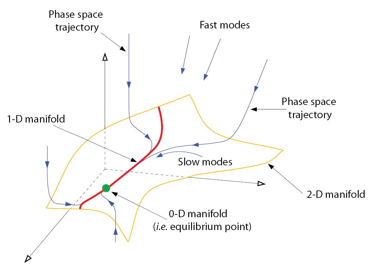
Many model reduction methods exploit this for simplifying chemical kinetics via a time scale separation into fast and slow modes. The aim is to approximate the system dynamics with a dimension-reduced model after eliminating the fast modes by enslaving them to the slow ones via computation of slow attracting manifolds.

Very early model reduction approaches like the quasi steady-state (QSSA) and partial equilibrium assumption (PEA) [1] performed “by hand”, have set the course for modern numerical model reduction methods that automatically compute a reduced model without need for detailed expert knowledge of chemical kinetics by the user. Many of these modern techniques are explicitly or implicitly based on a time-scale analysis of the underlying ordinary differential equation (ODE) system with the purpose to identify a slow attracting manifold in phase space where – after a short initial relaxation period – the system dynamics evolve. For a comprehensive overview see e.g. [3] and references therein.

In 1992 Maas and Pope introduced the ILDM-method [4] which became very popular and widely used in the reactive flow community, in particular in combustion applications. Based on a singular perturbation approach, a local time-scale analysis is performed on the Jacobian of the system of ordinary differential equations modeling chemical kinetics. Fast time scales are assumed to be fully relaxed and after a suitable coordinate transformation fast variables are computed as a function of the slow ones by solving a nonlinear algebraic equation system. For recent developments and extensions of the ILDM method see e.g. [5] and references therein.

Another popular technique is computational singular perturbation (CSP) method proposed by Lam in 1985 [6, 7]. The basic concept of this method is a representation of the dynamical system in a set of “ideal” basis vectors such that fast and slow modes are decoupled. In contrast to ILDM and CSP some iterative methods came into application that are not based on explicit computation of a time scale separation, but rather an evaluation of functional equations suitably describing the central characteristics of a slow attracting manifold, for example invariance and stability. Examples are Fraser’s algorithm [8, 9, 10] and the method of invariant grids [11, 12, 3]. Other widely known and successful methods are the constrained runs algorithm [13, 14], the rate-controlled constrained equilibrium (RCCE) method [15], the invariant constrained equilibrium edge preimage curve (ICE-PIC) method [16, 17], and flamelet-generated manifolds [18, 19]. In [20] finite time Lyapunov exponents and vectors are analyzed for evaluation of timescale information. Mitsos et al. formulated an integer linear programming problem explicitely minimizing the number of species in the reduced model subject to a given error constraint [21].

It is obvious that non-local information on phase space dynamics has to be taken into account to get accurate approximations of slow attracting manifolds in the general case. Reaction trajectories in phase space that are solutions of the ODE system describing chemical kinetics and uniquely determined by their initial values bear such information. Based on Lebiedz’ idea to search for an extremum principle that distinguishes trajectories on or near slow attracting manifolds, we apply an optimization approach for computing such trajectories [22, 23]. Various optimization criteria have been suggested [24], systematically investigated and the trajectory-based approach has been extended to the computation of manifolds of arbitrary dimension via parameterized families of trajectories.

This paper derives and comprehensively discusses various geometrically motivated objective criteria for computing trajectories approximating slow attracting manifolds in chemical kinetics as a solution of an optimization problem. The corresponding objective functionals are supposed to implicitly incorporate essential characteristics of slow attracting manifolds related to a minimal remaining relaxation of chemical forces along trajectories on these manifolds. We consider the picture of abstract “dissipative chemical forces” imagined to drive the single elementary reaction steps [25]. Due to energy dissipation these forces successively relax while the chemical system is approaching equilibrium. The successive relaxation of these forces causes curvature in the reaction trajectories (in the sense of velocity change along the trajectory). A slow 1-D manifold in this picture would correspond to a minimally curved reaction trajectory along which the remaining relaxation of chemical forces is minimal while approaching chemical equilibrium.

In particular, we propose and motivate an optimization criterion suitably measuring curvature which is rooted in a thermodynamically motivated Riemannian geometry specifically defined for chemical reaction kinetics and based on the Second Law of Thermodynamics. This metric provides the phase space of chemical reaction kinetics with a geometry specifically capturing the structure of chemical kinetic systems [26].

The proposed model reduction method is automatic. The user has to provide only the desired dimension of the reduced model and the range of concentrations of the reaction progress variables supposed to parameterize the reduced model. For the application examples presented in this work, the numerical optimization algorithm shows fast convergence independent of the initial values chosen for numerical initialization. The optimization problems seem to be convex for the example systems presented in this paper (see “optimization landscapes” in Section 3.1.2 and 3.3.3) and would then have a unique solution corresponding to a global minimum of the objective functional. An advantage of the presented trajectory optimization approach over local time scale separation methods like QSSA and ILDM is the fact that it produces smooth manifolds and whole 1-D manifolds (trajectories) as a solution of a single run of the optimization algorithm. Methods based on explicit local time scale separation might yield non-smooth manifolds when the fast-slow spectral decomposition changes its structure. Furthermore, the formulation as an optimization problem assures results even under conditions where the time scale separation is small and many common model reduction methods fail or numerical solutions are difficult to obtain.

2 Trajectory-based optimization approach

As described in the introduction, the key of the method presented here is the exploitation of global phase space information contained in the behavior of trajectories on their way towards chemical equilibrium. This information can be used within an optimization framework for identifying suitable reaction trajectories approximating slow invariant and attracting manifolds (SIM). A suitable formulation as the numerical solution of an optimization problem assures the existence of a reduced model irrespective of assumptions on the time scale spectrum, its structure and the dimension of the reduced model and sophisticated optimization software can be used for the numerical solution of the problem. The central idea behind our approach is that the optimization criterion for the identification of suitable trajectories should represent the assumption that chemical forces are – under the given constraints – already maximally relaxed along trajectories on the slow attracting manifold. From the opposite point of view this means that the remaining relaxation of chemical forces along the trajectories is minimal while approaching chemical equilibrium. This means that the velocity change caused by chemical force relaxation is minimal which is intuitively close to the notion of a slow manifold. Various ideas for the formulation of suitable optimization criteria are conceivable.

Mathematically the basic problem can be formulated as

$$\min_{c(t)}\int_{0}^{t_{\textrm{f}}}\Phi\left(c(t)\right)\;\mathrm{d}t$$ (1a)

subject to

$$\frac{\mathrm{d}c(t)}{\mathrm{d}t} =f\left(c(t)\right)$$ (1b)

$$0 =g\left(c(0)\right)$$ (1c)

$$c_{k}(0) =c_{k}^{0},\qquad k\in I_{\text{fixed}}.$$ (1d)

The variables $c_{k}$ denote the concentrations of chemical species, and $I_{\mathrm{fixed}}$ is an index set that contains the indices of variables with fixed initial values (the so-called reaction progress variables) chosen to parameterize the reduced model, i.e. the slow attracting manifold to be computed. Thus, those variables representing the degrees of freedom within the optimization problem are the initial value concentrations of the chemical species $c_{k}(0),k\notin I_{\rm fixed}$. The process of determining $c^{0}_{k},k\notin I_{\rm fixed}$ from $c^{0}_{k},k\in I_{\rm fixed}$ is known as “species reconstruction” and represents a function mapping the reaction progress variables to the full species composition by determining a point on the slow attracting manifold. In our approach, species reconstruction is possible locally, i.e. without being forced to compute the slow attracting manifold as a whole. The system dynamics (chemical kinetics determined by the reaction mechanism) are described by (1b) and enter the optimization problem as equality constraints. Hence an optimal solution of (1) always satisfies the system dynamics of the full ODE system. Chemical element mass conservation relations that have to be obeyed due to the law of mass conservation are collected in the linear function $g$ in (1c). The initial concentrations of the reaction progress variables are fixed via the equality constraint (1d).

When asymptotically approaching the equilibrium point $c^{\mathrm{eq}}$, which is a stable fixed point attractor in a closed chemical system, the system dynamics become infinitely slow and equilibrium will never be reached exactly. By approximating the equilibrium point within a surrounding of small radius $\varepsilon>0$ for the concentration of chemical species (e.g. the reaction progress variables) by an additional constraint $|c_{k}(t_{\textrm{f}})-c_{k}^{\mathrm{eq}}|\leqslant\varepsilon$ (equilibrium composition: $c^{\mathrm{eq}}$), the free final time $t_{\textrm{f}}$ can be automatically determined within the optimization problem assuring that this additional inequality constraint is fulfilled. However, in practical applications it is usually sufficient to choose $t_{\textrm{f}}$ large enough for the final point of the integration to be close to equilibrium. The objective functional $\Phi(c(t))$ in (1a) characterizes the optimization criterion which will be discussed later in detail.

The key idea of our approach to model reduction in chemical kinetics is found in the fact that suitable trajectories can be used to span slow attracting invariant manifolds. The approximated SIM can then be used as a reduced model of the underlying ODE model, for example via a look-up table for points on the slow manifold. This reduced model is parametrized by the reaction progress variables (coordinate axes) which find a fully natural realization in our formulation as trajectory initial concentrations (1d).

2.1 Numerical Methods: Multiple Shooting in a Parametric Optimization Setting

The optimization problem (1) can be solved as a standard nonlinear optimization problems (NLP), for example via the sequential quadratic programming (SQP) method [27]. However, one has to decide how to treat the differential equation constraint and the objective functional. The easiest way is a decoupled iterative approach, a full numerical integration of the ODE model with the current values of the variables subject to optimization. This is called the sequential (or single shooting) approach since it fully decouples simulation of the model and optimization. However, it is often beneficial to have an “all at once” approach that couples simulation and optimization via discretization of the ODE constraint. This simultaneous approach has the advantage of introducing more freedom into the optimization problem since the differential equation model does not have to be solved exactly in each iteration of the optimization. A beneficial approach to couple the ODE constraint to the optimization is the multiple shooting method. Here, the time interval is subdivided into several multiple shooting intervals and additional degrees of freedom are introduced at the initial points of each interval. On each multiple shooting interval an independent initial value problem is solved via numerical integration. Additional “matching condition”-equality constraints at the level of the optimization problem assure continuity of the final solution trajectory between the multiple shooting subintervals. For all results in this paper the multiple shooting approach introduced by Bock and Plitt [28, 29] is used.

The SQP method basically can be interpreted as Newton’s method applied to the Karush–Kuhn–Tucker (KKT) necessary optimality conditions of the NLP (see e.g. [30]) and requires the computation of derivatives. For the numerical approximation of these derivatives by finite difference methods, along with the nominal ODE solution trajectory $n$ perturbed trajectories have to be computed, where $n$ is the dimension of the ODE system. To avoid the dependence of the resulting derivative on the adaptive discretization schemes of these trajectories provided by an automatic step size control in the numerical integration routine, the perturbed trajectories are evaluated on the same grid as the nominal trajectory. This approach is called internal numerical differentiation (IND) [31]. As the systems considered here are chemical reaction systems which are usually stiff systems, the integration itself is performed by DAESOL [32, 33], a multistep backward differentiation formula (BDF) differential algebraic equation (DAE) solver. For all computations presented in the results section of this paper, the software package MUSCOD-II [29, 34, 35] has been used.

For the computation of slow attracting manifolds of dimension larger than one, a sequence of problems of type (1) has to be solved for different initial values of the reaction progress variables in (1d). For this purpose, we use a parametric optimization framework, where neighboring problems are efficiently initialized with the previous optimal solution. Through this continuation method embedding the problem into a parametric family of optimization problems, the computation of a family of optimal trajectories spanning a higher-dimensional manifold can be significantly accelerated. Such embedding strategy was originally developed and implemented into the package MUSCOD-II by Diehl et al. in [36, 37] for fast online optimization, especially real-time optimal control. A variant of this implementation has been used for the results presented in this paper.

2.2 Optimization criteria

Naturally, the choice of the criterion $\Phi(c(t))$ crucially affects both success and degree of accuracy of the computed approximations of the slow attracting manifold. A useful criterion $\Phi(c(t))$ should at least fulfill the following three requirements:

1. $\Phi$ should be physically motivated and describe in a suitable sense the extent of relaxation of “chemical forces” or “dynamical modes” in the evolution of reaction trajectories towards equilibrium.

2. $\Phi$ should be computable from easily accessible data contained in standard models of chemical reaction mechanisms (e.g. reaction rates, chemical source terms and their derivatives, thermodynamic data).

3. $\Phi$ should be twice continuously differentiable along reaction trajectories.

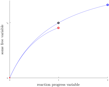
Another desirable but not necessary property, which is related to the invariance of a manifold is the following consistency property. If a criterion is consistent in the sense of the following definition, the manifold computed as a solution of the optimization problem is positively invariant which means that trajectories starting on the manifold at time $t_{0}$ will stay on the manifold for all $t\geqslant t_{0}$.

Definition 1 (Consistency property)

Suppose an optimal trajectory $\tilde{c}(t)$ has been computed as a solution of (1). Take the concentrations of the progress variables $\tilde{c}(t_{1})$ at some time $t_{1}>0$ as new initial concentrations for (1d) and solve (1) again. If $\hat{c}(t)=\tilde{c}(t+t_{1})$ holds for the resulting optimal trajectory $\hat{c}(t)$, we call the optimization criterion $\Phi$ consistent.

The consistency property, illustrated in Fig. 2, can be used as an accuracy test for the computed manifold, because the correct attracting SIM should be invariant by definition. However, it poses a strong demand that is not a priori incorporated into the problem formulation (1) and will not be fulfilled in general for solutions of the optimization problem. Nevertheless, an invariant manifold can in principle be constructed in our approach even without a consistent criterion by solving (1) for initial values $c_{k}^{0},\;k\in I_{\mathrm{fixed}}$ on the boundary of a desired domain and spanning the low-dimensional manifold by the resulting trajectories.

Figure 2: Illustration of the consistency property: An optimization problem has been solved for a fixed value (=$2.0$ here) for the progress variable. Its solution is the trajectory $\tilde{c}(t)$ starting from the blue circle and converging towards equilibrium (here the coordinate origin, red dot). At a later point in time $t_{1}>0$, the progress variable is fixed to the value on the trajectory $\tilde{c}_{k}(t)$ (=$1.0$ here), $k\in I_{\rm fixed}$, and the optimization problem is solved again. If the new solution $\hat{c}(t)$ coincides with the remaining part of the previous one such as the trajectory starting at the black circle, we call the criterion (1a) consistent, otherwise (e.g. the trajectory starting at the red circle) it is called inconsistent.

2.2.1 Curvature-based Relaxation Criteria

As pointed out before, a suitable optimization criterion $\Phi(c(t))$ should characterize the extent of relaxation of “chemical forces”. Fundamentally rooted criteria of this type can be derived on the basis of the concept of curvature of trajectories in phase space measured in a suitable metric. From a physical point of view curvature is closely related to the geometric interpretation of a force and its action on the system dynamics. This picture has a long historical tradition.

One of the most popular examples is Einstein’s general theory of relativity [38] which proposes the idea that gravitational force is replaced by a “geometric picture”. Einstein’s general theory of relativity relates the special theory of relativity and Newton’s law of universal gravitation with the insight that gravitation can be described by curvature of space-time. Space-time is treated as a four-dimensional manifold whose curvature is due to the presence of mass, energy, and momentum.

But even long before Einstein, the concept of curvature has already been related to the concept of force in physics. In 1687 Sir Isaac Newton published the laws of motion in his work “Philosophiae Naturalis Principia Mathematica”. In a differential formulation Newton’s second law can be stated as $F=m\cdot a,$ where $m$ is mass, $a$ is acceleration, and $F$ is force. Since the acceleration $a$ is the second derivative of the state variable $x(t)$ with respect to time, $a=\ddot{x}$, and thus contains information about the curvature of $x$; Newton’s law is the first one to directly relate force to curvature.

In this context it is important to remark that equations of motion in classical mechanics can also be described by a variational principle, Hamilton’s principle of least action. In Lagrange-Hamilton mechanics [39], the trajectory of an object is determined in such a way that the action (which is defined as the integral of the Lagrangian over time, where the Lagrangian is the difference of kinetic energy and potential energy) is minimal.

A central issue in this paper is to transfer the principle of “force = curvature” to the field of chemical systems and look for a corresponding variational principle characterizing the kinetics along a slow attracting manifold. In chemical systems dissipative forces are active. The different time scales of dynamic modes result in an anisotropic force relaxation in phase space. This force relaxation changes the reaction velocity. Inspired by an analogy observation with Newton’s geometric interpretation of a force as a second derivative of a trajectory with respect to time, we regard the second time-derivative of the chemical composition $c(t)$ characterizing the rate of change of reaction velocity through relaxation (dissipation) of chemical forces:

$$\dot{c}=f(c),\quad\ddot{c}=\frac{\mathrm{d}\dot{c}}{\mathrm{d}t}=\frac{\mathrm{d}\dot{c}}{\mathrm{d}c}\cdot\frac{\mathrm{d}c}{\mathrm{d}t}=J_{f}(c)\cdot f.$$ (2)

We consider the tangent (reaction velocity) vectors $\dot{c}(t)=f(c(t))$ of reaction trajectories. The relaxation of chemical forces results in a change of $\dot{c}(t)$ along a trajectory on its way towards chemical equilibrium. This change along the trajectory may be characterized by taking the directional derivative of the tangent vector of the curve $c(t)$ with respect to its own direction $v\coloneqq\frac{\dot{c}}{\|\dot{c}\|_{2}}=\frac{f}{\|f\|_{2}}$. Mathematically this can be formulated as

$$D_{v}\dot{c}(t)\coloneqq\frac{\mathrm{d}}{\mathrm{d}\alpha}f(c(t)+\alpha v)\Big{|}_{\alpha=0}=J_{f}(c)\cdot\frac{f}{\|f\|_{2}},$$

with $J_{f}(c)$ being the Jacobian of the right hand side $f$ evaluated at $c(t)$ and $\|\cdot\|_{2}$ denoting the Euclidian norm. Hence, we may choose the optimization criterion

$$\Phi_{\textrm{A}}(c)=\frac{\|J_{f}(c)\;f\|_{2}}{\|f\|_{2}}$$ (3)

in the formulation (1a). This criterion bears some resemblance to the recently published method of stretching-based diagnostics [40] and its application for model reduction (SBR-method). The authors use an expression closely related to criterion (3) which measures the stretching of vector fields in the tangent bundle of manifolds.

The natural way for the evaluation of criterion (3) in the formulation of the objective functional (1a) would be a path integral along the trajectory towards equilibrium

$$\int_{l(0)}^{l(t_{\textrm{f}})}\Phi(c(l(t)))\;\mathrm{d}l(t),$$

where $l(t)$ is the Euclidian length of the curve $c(t)$ at time $t$ given by

$$l(t)=\int_{0}^{t}\|\dot{c}(\tau)\|_{2}\;\mathrm{d}\tau.$$

This results in the reparametrization

$$\mathrm{d}l(t)=\|\dot{c}(t)\|_{2}\;\mathrm{d}t.$$ (4)

The objective used in (1a) would be (using (2)):

$$\int_{0}^{t_{\textrm{f}}}\|J_{f}(c)\;f\|_{2}\;\mathrm{d}t=\int_{0}^{t_{\textrm{f}}}\|\ddot{c}\|_{2}\;\mathrm{d}t.$$ (5)

However, an alternative norm for the evaluation of $\|J_{f}(c)\;f\|$ might be taken into account, which has already been used by Weinhold in [41] and is motivated from thermodynamics. This norm is also known as Shashahani norm [42] and is employed for model reduction purposes in [26]. In this norm the criterion adapted from (3) can be written as

$$\Phi_{\textrm{B}}(c)=\frac{\|J_{f}(c)\;f\|_{W}}{\|f\|_{W}}=\frac{(f^{\textrm{T}}J_{f}^{\textrm{T}}(c)\cdot\mathrm{diag}(1/c_{i})\cdot J_{f}(c)f)^{1/2}}{(f^{\textrm{T}}\cdot\mathrm{diag}(1/c_{i})\cdot f)^{1/2}}$$ (6)

with $W=\mathrm{diag}(1/c_{i})$ being the diagonal matrix with diagonal elements $1/c_{i}$. This criterion brings thermodynamic considerations into play and represents the Riemannian geometry induced by the second differential of Gibbs free enthalpy $G$

$$G=\sum_{i=1}^{n}c_{i}[\ln(c_{i}/c_{i}^{\mathrm{eq}})-1],\ \ W=\mbox{Hess}(G).$$

It measures the thermodynamic anisotropy of the phase space by weighting the coordinate axis corresponding to species $i$ with the gradient $\frac{\partial\mu_{i}}{\partial c_{i}}=\mbox{Hess}(G)_{i,i}$ of the chemical potential $\mu_{i}=\frac{\partial G}{\partial c_{i}}$ of species $i$ in that direction. The corresponding metric has been discussed in the context of an entropic scalar product [26]. The corresponding objective function in the general optimization problem (1) for the $W$-norm would be

$$\int_{0}^{t_{\textrm{f}}}\|J_{f}(c)\;f\|_{W}\;\mathrm{d}t.$$ (7)

Interestingly, from a different point of view the objective functionals (5) and (7) can also be interpreted as minimizing the length of a trajectory in a suitable Riemannian metric. For any continuously differentiable curve $\gamma(t)$ on a Riemannian manifold, the length $L$ of $\gamma$ is defined as

$$L(\gamma)=\int_{\gamma}\sqrt{g_{\gamma(t)}(\dot{\gamma}(t),\dot{\gamma}(t))}\;{\rm d}t$$ (8)

with $g_{\gamma(t)}$ being a scalar product defined on the tangent space of the curve in each point. The Riemannian metric $g_{\gamma(t)}$ might be chosen as

$$g_{\gamma(t)}(f,f)\coloneqq f^{\textrm{T}}\;{J^{\textrm{T}}_{f}(c)\cdot A\cdot J_{f}(c)}\;f\;=\;\|J_{f}(c)\;f\|_{A}^{2},$$ (9)

for a positive definite matrix $A$. The “length-minimizing” objective functional equivalent to criterion (1a) is now

$$\min\;L(\gamma)$$ (10)

subject to constraints (1b)–(1d). With the solution trajectory of this problem, the “minimum distance from equilibrium in a kinetic sense” can be formulated in an explicit mathematical form based on concepts from differential geometry. In [24], a heuristic choice for a matrix $A$ was made based on the entropy production rate. However, the results achieved using the norm proposed in (6) yield more accurate results for the computation of slow attracting manifolds in chemical kinetics. Another heuristic interpretation of (5) is possible based on the fact that the time-integral over a rate of change of velocity is time-averaged velocity whose minimum is intuitively related to the notion of a slow manifold.

2.2.2 Geometric curvature of curves in space

In the face of our central aim to relate the principle “force equals curvature” to model reduction for chemical kinetics we refer to some mathematical definitions and properties of curvature in this section. Various concepts and corresponding definitions of curvature of manifolds and curves in $\mathbb{R}^{n}$ can bee found in general literature on differential geometry as e.g. [43, 44, 45].

Let $\bar{c}:J=(0,L)\rightarrow\mathbb{R}^{n}$ be a curve defined on an open interval $J\subset\mathbb{R}$ and parameterized by arc length $s$, meaning $\left\|\frac{\mathrm{d}}{\mathrm{d}s}\bar{c}(s)\right\|_{2}=1$ ($\|\cdot\|_{2}$ denoting the Euclidian norm). The value of $\left\|\frac{\mathrm{d}^{2}}{\mathrm{d}s^{2}}\bar{c}(s)\right\|_{2}$ is a measure for the rate, how rapidly the curve pulls away from its tangent in a neighborhood of $\bar{c}(s)$. That leads directly to the following definition.

Definition 2 (Curvature)

Let $\bar{c}:J\rightarrow\mathbb{R}^{n}$ be a curve parametrized by arc length $s\in J$. The number

$$\kappa(s)\coloneqq\left\|\frac{\mathrm{d}^{2}}{\mathrm{d}s^{2}}\bar{c}(s)\right\|_{2}$$

is called curvature of a curve $\bar{c}$ at $s$ (or at $\bar{c}(s)$).

However, in general trajectories in chemical composition space regarded as curves in vector space are not parameterized in arc-length, but e.g. time $t$. We want to compute the curvature for the case of an arbitrary parametrization $t$. Let $c:I\rightarrow\mathbb{R}^{n}$ be a regular curve, $I,J\subset\mathbb{R}$ open, $\varphi:J\rightarrow I$ the diffeomorphism resulting in $\bar{c}\coloneqq c\circ\varphi$ being parametrized in arc length with w.l.o.g. $\varphi(s)>0\ \forall s\in J$. Then

$$\frac{\mathrm{d}}{\mathrm{d}s}\bar{c}(s)=\frac{\mathrm{d}}{\mathrm{d}\varphi(s)}c(\varphi(s))\frac{\mathrm{d}}{\mathrm{d}s}\varphi(s)$$ (11)

and

$$\frac{\mathrm{d}^{2}}{\mathrm{d}s^{2}}\bar{c}(s)=\frac{\mathrm{d}^{2}}{\mathrm{d}\varphi(s)^{2}}c(\varphi(s))\left(\frac{\mathrm{d}}{\mathrm{d}s}\varphi(s)\right)^{2}+\frac{\mathrm{d}}{\mathrm{d}\varphi(s)}c(\varphi(s))\frac{\mathrm{d}^{2}}{\mathrm{d}s^{2}}\varphi(s)$$ (12)

hold. As $\bar{c}$ is parametrized in arc length (11) leads to

$$\frac{\mathrm{d}}{\mathrm{d}s}\varphi(s)=\frac{1}{\left\|\frac{\mathrm{d}}{\mathrm{d}\varphi(s)}c(\varphi(s))\right\|_{2}}.$$

For the second derivative of $\varphi$, that appears in (12), the application of the chain rule yields (with $\langle\cdot,\cdot\rangle_{2}$ being the Euclidian scalar product)

$$\frac{\mathrm{d}^{2}}{\mathrm{d}s^{2}}\varphi(s)=-\frac{\left\langle\frac{\mathrm{d}}{\mathrm{d}\varphi(s)}c(\varphi(s)),\frac{\mathrm{d}^{2}}{\mathrm{d}\varphi(s)^{2}}c(\varphi(s))\right\rangle_{2}}{\left\|\frac{\mathrm{d}}{\mathrm{d}\varphi(s)}c(\varphi(s))\right\|_{2}^{4}}.$$

Bringing the last two formulae together with (12) and $t=\varphi(s)$ we arrive at the formula for the curvature of $c(t)$:

$$\kappa(t)\coloneqq\Phi_{\textrm{C}}(c(t))\coloneqq\left\|\frac{\ddot{c}(t)}{\|\dot{c}(t)\|_{2}^{2}}-\langle\dot{c}(t),\ddot{c}(t)\rangle_{2}\frac{\dot{c}(t)}{\|\dot{c}(t)\|_{2}^{4}}\right\|_{2}.$$ (13)

Recalling the discussions in the last section, an alternative optimization criterion for (1a) could be the curvature (13). In this context the total (integrated) curvature should be the objective function in (1):

$$\kappa_{\rm tot}\coloneqq\int_{l(0)}^{l(t_{\text{f}})}\kappa(s)\mathrm{d}s,$$

which can be expressed in time-parameterization as

$$\kappa_{\rm tot}=\int_{0}^{t_{\mathrm{f}}}\kappa(t)\|\dot{c}(t)\|_{2}\;\mathrm{d}t=\int_{0}^{t_{\mathrm{f}}}\left\|\frac{\ddot{c}(t)}{\|\dot{c}(t)\|_{2}}-\langle\dot{c}(t),\ddot{c}(t)\rangle_{2}\frac{\dot{c}(t)}{\|\dot{c}(t)\|_{2}^{3}}\right\|_{2}\mathrm{d}t$$ (14)

with $\kappa(t)$ as in equation (13).

Intuitively, the local curvature of a trajectory on its way to equilibrium in phase space should have a peak each time it relaxes onto a lower dimensional manifold. Therefore, also this criterion is related to the relaxation of chemical forces in some sense.

2.2.3 Evaluation of the Objective Functional

From a practical perspective, the computation of the Jacobian for the expression of the different criteria is not necessary, as $\ddot{c}(t)=J_{f}(c(t))\;f(c(t))$ simply is a directional derivative of the ODE vector field with respect to its own direction. This directional derivative could be evaluated using classical difference quotients [46], but a more appealing alternative is found in [47]. Instead of using the central difference formula

$$F^{\prime}(x_{0})\approx\frac{F(x_{0}+\delta)-F(x_{0}-\delta)}{2\delta}$$ (15)

for the approximation of the derivative of the real valued function $F(x)$, Squire and Trapp [47] suggest replacing $\delta$ with $\mathrm{i}\delta$ ($\mathrm{i}=\sqrt{-1}$). If $F$ is an analytic function, (15) then reads

$$F^{\prime}\approx\frac{\Im[{F(x_{0}+\mathrm{i}\delta)}]}{\delta},$$ (16)

with $\Im(z)$ being the imaginary part of $z$. This is called complex-step derivative approximation. This result is especially appealing, as (16) does not contain a subtraction and hence eliminates cancellation errors. Therefore $\delta$ can be chosen very small, hence making higher-order terms in the Taylor expansion negligible. For the directional derivative $\ddot{c}$ at a point $c_{0}$ with $c$ from $\dot{c}=f(c)$, (16) reads

$$\ddot{c}|_{c_{0}}\approx\frac{\Im[f(c+\mathrm{i}\delta f(c))]}{\delta}.$$ (17)

Compared to the use of the full Jacobian, the complexity for the evaluation of $\ddot{c}$ can be reduced from $\mathcal{O}(n^{2})$ to $\mathcal{O}(n)$ using this complex variable approach. At the same time a high accuracy is guaranteed by the possibility of using an extremely small $\delta$.

However, a numerical difficulty occurs for the evaluation of the objectives (7) and (14). In case of (7) the weights for the $W$-norm are obtained as inverted species concentrations. Especially for radical species the denominator becomes generally very small near chemical equilibrium resulting in numerical instabilities. The case of (14) is even more difficult, as negative exponents $>1$ occur for the norm of the reaction rates. Near the equilibrium point the reaction rates become infinitesimally small and this results in severe numerical problems. A remedy for this problem is an additional equality constraint. Instead of fixing the final time $t_{\textrm{f}}$ at a large value, it can be left free in the optimization determined by an end point constraint

$$\|f(c(t_{\textrm{f}}))\|_{2}=\epsilon$$ (18)

with a sufficiently large $\epsilon$ keeping the end point of the trajectory away from equilibrium.

3 Results

In this section, results for our model reduction method based on trajectory optimization are presented. We choose three different chemical reaction mechanisms to demonstrate its application: the Davis–Skodje model system, a simplified reaction mechanism for the combustion of H₂, and a realistic temperature dependent mechanism for ozone decomposition. For these three mechanisms all previously discussed objective functionals (5), (7), and (14) in the general problem (1) are tested for the purpose of numerically computing approximations of slow attracting manifolds. The results are compared and discussed.

3.1 The Davis–Skodje Test Problem

The well-known Davis–Skodje mechanism is our first test case [8, 48].

$$\frac{\mathrm{d}y_{1}}{\mathrm{d}t}=-y_{1},\quad\frac{\mathrm{d}y_{2}}{\mathrm{d}t}=-\gamma y_{2}+\frac{(\gamma-1)y_{1}+\gamma y_{1}^{2}}{(1+y_{1})^{2}},$$

where $\gamma>1$ is a measure for the spectral gap or stiffness of the system. Typically model reduction algorithms show a good performance for large values of $\gamma$, which represent a large gap between the time scales of fast and slow modes. Small values of $\gamma$ impose a significantly harder challenge on the computation of slow attracting manifolds. For reasons of adjustable time scale separation and analytically computable slow invariant manifold and ILDM, the Davis–Skodje model is widely used for testing numerical model reduction approaches.

3.1.1 Results for Different Optimization Criteria

In Figures 3, 4, and 5 results for criteria (5), (7), and (14) respectively are depicted.

Figure 3: Results for the Davis–Skodje problem with (5) as objective functional. Results for different values of $\gamma$ are shown. The red curve is the analytically computed SIM. The black dashed curve represents the analytic Maas–Pope-ILDM. The blue curves are trajectories numerically integrated from those initial points that are solutions of our optimization problem.

Figure 4: Results for the Davis–Skodje problem with (7) as objective functional. Again, results for different values of $\gamma$ are shown together with the SIM (red) and the Maas–Pope-ILDM (black, dashed).

Figure 5: Results for the Davis–Skodje problem with (14) as objective function. Only results for $\gamma=6.0$ are shown, cf. the discussion in Section 3.1.2 including Figures 6(a) and 6(b).

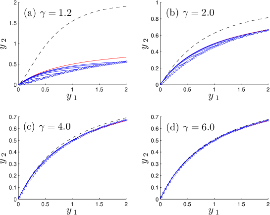
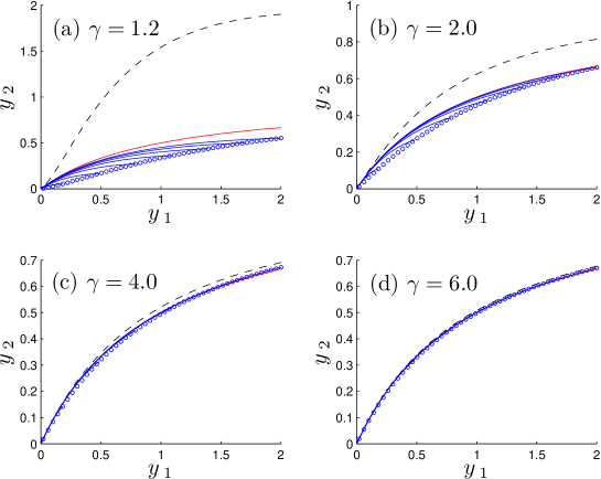
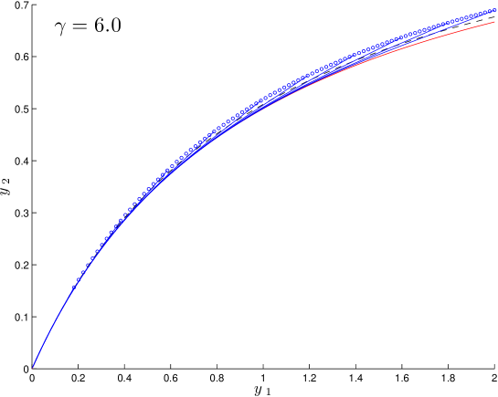
We will refer to criterion (3) as criterion A in the following. The dependence of the accuracy of the computed slow attracting manifold on the stiffness parameter $\gamma$ becomes obvious. In all cases, the value of $y_{1}$ is fixed as reaction progress variable. The optimization problem is solved repeatedly for different values for $y_{1}$. For large and moderate values of the stiffness parameter, good approximations of the SIM (red) are achieved. For $\gamma=1.2$ the results become more inaccurate. For comparison the Maas–Pope-ILDM is plotted as dashed black line, it can be computed analytically for the Davis–Skodje model [8]. The computational effort for one solution of the optimization problem is on average about twelve SQP-iterations (cf. Section 2.1) which takes about ten seconds in total on a single core Intel^® Pentium^® 4 (3 GHz)-machine with 2 GB memory. Of course, the convergence time (not the result) depends on the initial values chosen to start the numerical algorithm. We use a non-equidistant multiple shooting grid with twenty intervals. The number of evaluations of the function $f$ is of order $10^{5}$, the order of the number of matrix factorizations is $10^{4}$. Due to the parametric optimization strategy and application of initial value embedding [36, 37] pointed out in Section 2.1, every follow-up solution of a neighboring problem with slightly different values for the reaction progress variables needs only three to five SQP-iterations.

For the second criterion (7) – denoted B in the following – the results look very similar (see Fig. 4). As in the Davis–Skodje model the values for the variables $y_{1}$ and $y_{2}$ are of the same order, this is obvious considering the scaling in criterion (6). Results for criterion C (14), the total curvature, are shown in Figure 5. With this criterion, we could not obtain reasonable results for values of $\gamma<6.0$ which will be further explained in the next section.

3.1.2 Optimization Landscapes

Since the Davis–Skodje test problem consists of only two variables, the structure of optimization landscapes can easily be visualized. To compute these landscapes, the initial values of both variables are varied over a fixed range and for the trajectories starting in each of these pairs of initial values, the values of (5), (7), or (14) respectively are calculated. These objective functional values are depicted as a function of the initial values of the corresponding trajectories. Calculations are performed and plots are generated using MATLAB^®.

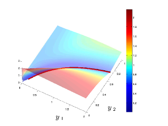
For the Davis–Skodje problem, we restrict ourselves to the illustration of criterion C, where we did not achieve satisfying results for small values of $\gamma$ (see previous subsection). In Figure 6(a) the results for $\gamma=6.0$ are shown. Additionally the SIM (red) and the ILDM (black) are projected onto the optimization landscape. Remember, that in our approach for a fixed value of $y_{1}$ the minimum of the objective value identifies the corresponding initial value of $y_{2}$.

(a) Results with $\gamma=6.0$ corresponding to results depicted in Fig. 5.

(b) Results with $\gamma=2.0$. No minimum near the SIM can be found.

Figure 6: Optimization landscape for the Davis–Skodje-model. The integrated (total) curvature (14) is plotted on the $z$-axis and coded in color for illustration reasons. The analytically computed SIM (red) and the analytically given Maas–Pope-ILDM (black) are projected onto the landscape.

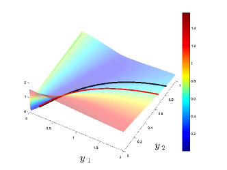
An optimization landscape for $\gamma=2.0$ and criterion C is shown in Figure 6(b). In this case, the criterion fails. No minimum can be found in the neighborhood of the SIM. The reason for this is that obviously for small time scale separation the relation between geometric and kinetic properties of the trajectories pointed out in Section 2.2.2 becomes weaker and linear segments of trajectories are preferred in the optimization objective functional against a slow attracting manifold (see “valley” in Fig. 6(b)). As explained in Section 2.2.2, criterion C measures the curvature generated through relaxation of a trajectory onto a slow attracting manifold. Thus, if relaxation is weak, the criterion becomes inaccurate.

3.2 Model Hydrogen Combustion Reaction Mechanism

In this section we consider a small test mechanism, which has been used for model reduction purposes in [49, 26, 24]. It consists of six chemical species involved in six (in each case forward and backward) elementary reactions involving two element mass conservation relations for hydrogen and oxygen (cf. Table 1).

Table 1: Simple hydrogen combustion test mechanism from [26]. Forward and backward rate constants are given temperature-independently.

Reaction $k_{+}$ $k_{-}$ $\mathrm{H_{2}}$ $\rightleftharpoons$ $\mathrm{2}\,\mathrm{H}$ $2.0$ $216.0$ $\mathrm{O_{2}}$ $\rightleftharpoons$ $\mathrm{2}\,\mathrm{O}$ $1.0$ $337.5$ $\mathrm{H_{2}O}$ $\rightleftharpoons$ $\mathrm{H}+\mathrm{OH}$ $1.0$ $1400.0$ $\mathrm{H_{2}}+\mathrm{O}$ $\rightleftharpoons$ $\mathrm{H}+\mathrm{OH}$ $1000.0$ $10800.0$ $\mathrm{O_{2}}+\mathrm{H}$ $\rightleftharpoons$ $\mathrm{O}+\mathrm{OH}$ $1000.0$ $33750.0$ $\mathrm{H_{2}}+\mathrm{O}$ $\rightleftharpoons$ $\mathrm{H_{2}O}$ $100.0$ $0.7714$

With the mass conservation relations

$$\begin{split}2\>c_{\text{H}_{2}}+2\>c_{\text{H}_{2}\text{O}}+c_{\text{H}}+c_{\text{OH}}&=C_{1}\\ 2\>c_{\text{O}_{2}}+c_{\text{H}_{2}\text{O}}+c_{\text{O}}+c_{\text{OH}}&=C_{2}\end{split}$$

this mechanism yields a system with four degrees of freedom. For our computations $C_{1}=2.0$ and $C_{2}=1.0$ were chosen.

3.2.1 One-dimensional Manifolds

We first present results for the computation of one-dimensional manifolds in composition space. The value of $c_{\text{H}_{2}\text{O}}$ serves as reaction progress variable. It is varied between 0.05 and 0.65. We present and compare results for the three different optimization criteria introduced in Section 2.2.1. In general, for testing accuracy of model reduction approaches it is very difficult to provide qualitative and quantitative measures of accuracy of numerical results. The reason for this is the nonavailability of (analytical) expressions for a SIM. Commonly we consider “eye inspection” of trajectory bundling behavior as well as consistency (invariance) as a qualitative measure of accuracy.

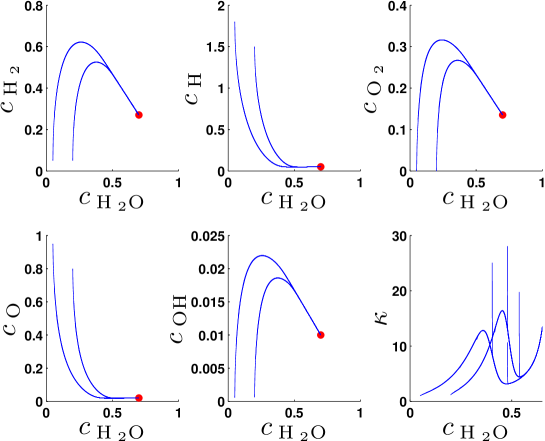
In Figure 7, results for criterion A are shown. The values of the free variables computed in the optimization are plotted versus the value of $c_{\text{H}_{2}\text{O}}$. Especially for the radical species concentrations $c_{\text{H}}$ and $c_{\text{O}}$ criterion A turns out to be inconsistent to some extent in the sense of Definition 1.

Figure 7: Results for the hydrogen combustion mechanism with criterion A. The free variables and the integrand of the objective functional are plotted versus the reaction progress variable $c_{\mathrm{H}_{2}\mathrm{O}}$. For different values of $c_{\mathrm{H}_{2}\mathrm{O}}$ the optimization problem is solved and the evolution of the resulting trajectories (blue curves) towards equilibrium (red dot) is shown. Especially for the radical species concentrations $c_{\mathrm{H}}$ and $c_{\mathrm{O}}$ criterion A turns out to be inconsistent.

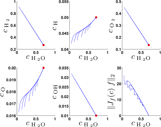
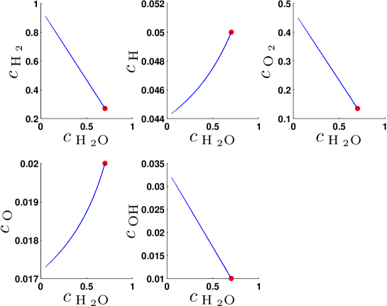
Figure 8 shows the results for the weighted criterion B. A significant improvement towards better consistency is achieved.

Figure 8: Results for the hydrogen combustion mechanism with criterion B.

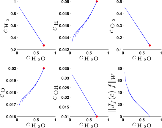
The third criterion C which failed in case of the Davis–Skodje test problem here performs best, cf. Figure 9. The results are nearly consistent. For criterion C the additional equality constraint (18), proposed in Section 2.2.3 has been used to prevent numerical instabilities near the equilibrium point. The computational effort for a 1-D manifold is in the order of seconds.

Figure 9: Results for the hydrogen combustion mechanism with criterion C.

3.2.2 Two-dimensional Manifolds

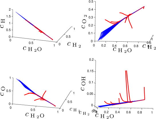
As the hydrogen combustion model has four degrees of freedom, also two-dimensional manifolds can be constructed. In the presented examples, $c_{\text{H}_{2}\text{O}}$ and $c_{\text{H}_{2}}$ serve as reaction progress variables. We present consistency tests plotted in two dimensions and finally show three-dimensional plots of the computed two-dimensional manifold and the relaxation of trajectories started from arbitrary initial values onto this 2-D manifold.

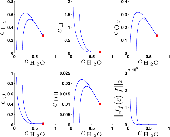
Figure 10 refers to criterion A. The resulting trajectories are plotted. After some time $t_{1}$ the values of the progress variables are fixed and the problem is solved again for testing consistency by eye inspection which turns out to be quite accurate. For criterion B (see Fig. 11), comparably good consistency is observed.

Figure 10: Results for a two-dimensional manifold for the hydrogen combustion mechanism with criterion A. The values of the progress variables are fixed to $0.05$ and $0.2$ in case of $c_{\mathrm{H}_{2}\mathrm{O}}$ and to $0.05$ in case of $c_{\mathrm{H}_{2}}$. Consistency tests are performed.

Figure 11: Results for a two-dimensional manifold for the hydrogen combustion mechanism with criterion B. The results are comparable to the results for criterion A, cf. Figure 10.

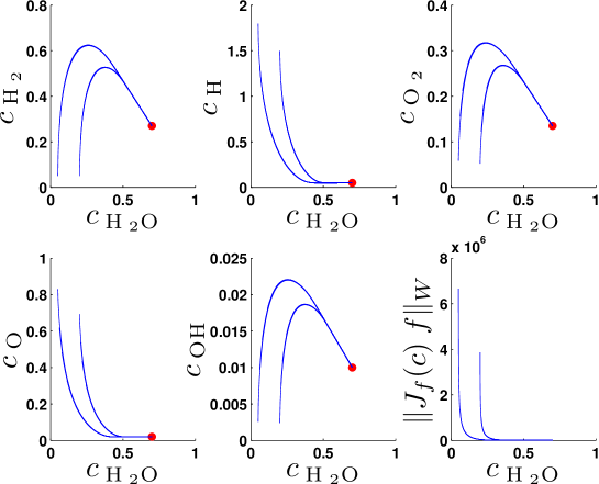
Results for the third criterion C are depicted in Figure 12. Here the peaks in the curvature during relaxation onto a lower-dimensional manifold mentioned in Section 2.2.2 become obvious.

Figure 12: Results of the two-dimensional manifold for the hydrogen combustion mechanism using criterion C.

For visualization of the two-dimensional manifold, three-dimensional cuts of six-dimensional composition space are plotted in Figure 13. The remaining free variables are plotted versus the reaction progress variables. Arbitrary trajectories relax on the 2-D manifold spanned by the computed trajectories. The computational effort for a 2-D manifold is in the order of some minutes.

Figure 13: Three-dimensional plots of the two-dimensional manifold for the hydrogen combustion mechanism. The free variables are plotted versus the progress variables. The manifold is spanned by trajectories (blue) computed for initial fixed values $c_{k}^{0}$ with criterion C as objective functional. Arbitrary trajectories (red) fulfilling the element mass conservation are computed to visualize their relaxation onto the manifold.

3.3 Ozone Decomposition Reaction Mechanism

Our last test case is a three component ozone decomposition mechanism (see Table 2) taken from [50]. It has been chosen to demonstrate the performance of our method taking temperature dependence via Arrhenius kinetics into account. Many model reduction approaches explicitly based on time scale separation fail when the spectral gap between fast and slow modes becomes too small which is often the case for low temperatures.

Table 2: Ozone decomposition mechanism from [50]. Rate coefficient $k=AT^{b}\exp(-E_{\mathrm{a}}/RT)$. Collision efficiencies in reactions including $\mathrm{M}$: $f_{\rm O}=1.14,f_{{\rm O}_{2}}=0.40,f_{{\rm O}_{3}}=0.92$.

Reaction $A$ / $\text{cm},\text{mol},\text{s}$ $b$ $E_{\mathrm{a}}$ / $\frac{\text{kJ}}{\text{mol}}$ O + O + M $\rightarrow$ O₂ + M $2.90\times 10^{17}$ $-1.0$ $0.0$ O₂ + M $\rightarrow$ O + O + M $6.81\times 10^{18}$ $-1.0$ $496.0$ O₃ + M $\rightarrow$ O + O₂ + M $9.50\times 10^{14}$ $0.0$ $95.0$ O + O₂ + M $\rightarrow$ O₃ + M $3.32\times 10^{13}$ $0.0$ $-4.9$ O + O₃ $\rightarrow$ O₂ + O₂ $5.20\times 10^{12}$ $0.0$ $17.4$ O₂ + O₂ $\rightarrow$ O + O₃ $4.27\times 10^{12}$ $0.0$ $413.9$

The ozone decomposition mechanism involves the element mass conservation relation

$$c_{\text{O}}+2\>c_{\text{O}_{2}}+3\>c_{\text{O}_{3}}=C$$

leaving a system with two degrees of freedom. We choose without loss of generality $C=1$.

3.3.1 Results for Different Optimization Criteria

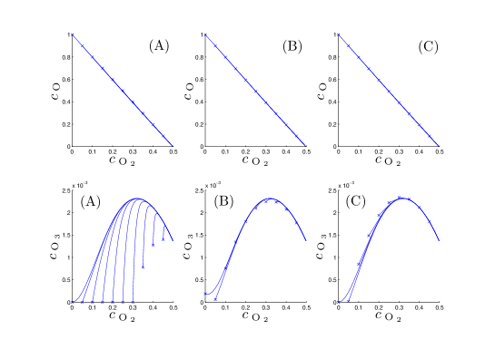
The ozone decomposition model has two degrees of freedom and we compute one-dimensional manifolds. The results for different temperatures are compared. Consistency tests are performed as in the previous sections. For criterion A at $T=1000~{}{\textrm{K}}$ (Fig. 14), a short relaxation phase of the computed trajectories can be observed, indicating inconsistency. The other criteria yield more consistent results and seem to be of comparable quality for approximation of a slow attracting manifold.

Figure 14: Results for the ozone decomposition mechanism at a temperature of $T=1000~{}{\mathrm{K}}$ with the three different criteria A (left), B (middle), and C (right). The free variables are plotted versus $c_{\mathrm{O}_{2}}$ as reaction progress variable. The optimization problem is solved several times with different values of $c_{\mathrm{O}_{2}}(0)$ (x-marks depicting the initial values of the optimal solution trajectories). The solution trajectories starting at the blue x-marks are shown on their way to equilibrium ($c_{\mathrm{O}_{2}}^{\mathrm{eq}}=0.5$). All criteria work reasonably well, but criterion A is worse concerning consistency.

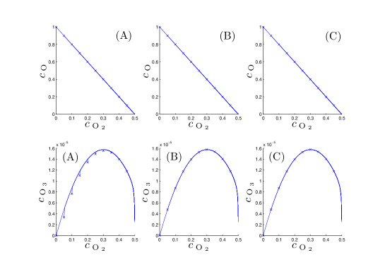
For a lower temperature of $T=500~{}{\textrm{K}}$ (Figure 15), criterion A obviously fails for the “relatively small” absolute values of $c_{\text{O}_{3}}$, whereas criteria B and C yield good approximations of the SIM.

Figure 15: Results for the ozone decomposition mechanism at a temperature of $T=500~{}{\mathrm{K}}$ with the three different criteria arranged as in Figure 14. Criteria B and C perform well, whereas criterion A obviously fails.

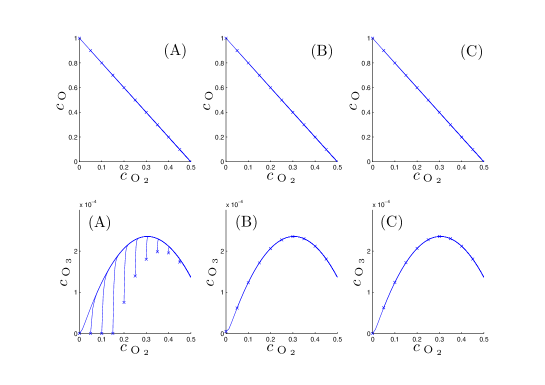
For $T=350~{}{\textrm{K}}$, the effects observed in Figure 15 amplify. However, according to the results shown in Figure 16 criteria B and C still perform reasonably well in this low-temperature region.

Figure 16: Results for the ozone decomposition mechanism at a temperature of $T=350~{}{\mathrm{K}}$.

3.3.2 Comparison with ILDM

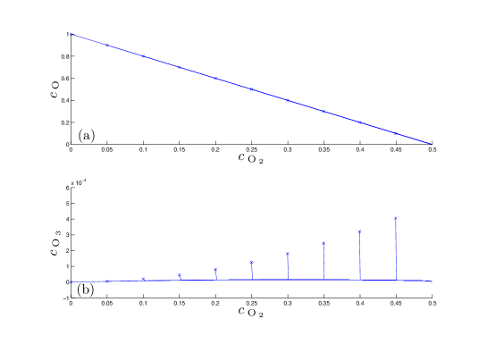
For the ozone decomposition mechanism we make a comparison of our results at $T=1000~{}{\mathrm{K}}$ with the ILDM method [4]. We numerically compute ILDM-points for a range of $c_{\mathrm{O}_{2}}$ values. Figure 17 depicts the results. A comparison of Figure 17(b) with the lower row of Figure 14 demonstrates a significantly better performance of our trajectory optimization method. The ILDM points do not lie close to the slow attracting manifold.

Figure 17: Results of the ILDM computation for the ozone decomposition mechanism at a temperature of $T=1000~{}{\mathrm{K}}$. The x-marks depict the ILDM-points. They have been computed with the code used in [2], accuracy tolerance $10^{-9}$ for the solution of the ILDM-equation via Newton’s method. The computation of ILDM points is initialized with the solution points of the optimization method using criterion B, cf. Fig. 14. Blue lines: trajectories started in the x-marks.

3.3.3 Optimization Landscapes

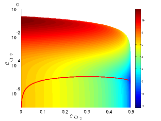
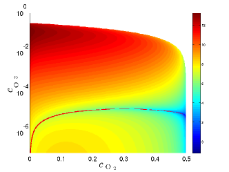
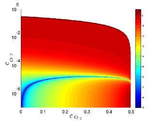
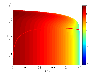
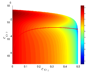
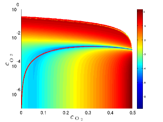
We compute optimization landscapes for the ozone decomposition model which has two degrees of freedom. Initial values for $c_{\mathrm{O}_{2}}$ and $c_{\mathrm{O}_{3}}$ are varied within the physically allowed range. The value of the objective function is computed for trajectories corresponding to tuples of initial values and depicted via color coding in a logarithmic scale. We compare these optimization landscapes for $T=1000~{}{\mathrm{K}}$ and $T=350~{}{\mathrm{K}}$.

Figure 18(a) shows the optimization landscape computed for criterion A ($T=1000~{}{\mathrm{K}}$). The other criteria, B and C, give rise to a much more distinct minimum of the objective function, cf. Figure 18(b) and 18(c). In the case of $T=350~{}{\mathrm{K}}$ criterion A fails, cf. Fig. 18(d), no minimum near the SIM is found. The distinct minima for criteria B and C become shallow but still allow for an optimal solution close to the SIM. Figures 18(e) and 18(f) correspond to criteria B and C respectively and visualize the results of the optimization problem presented in Section 3.3.1.

(a) Optimization landscape for the ozone decomposition mechanism at $T=1000~{}{\mathrm{K}}$. The color represents the value of (5) for criterion A.

(b) Optimization landscape for the ozone mechanism at $T=1000~{}{\mathrm{K}}$: The color represents the value of (7) for criterion B.

(c) Optimization landscape for the ozone mechanism at $T=1000~{}{\mathrm{K}}$: The color represents the value of (14) for criterion C.

(d) Optimization landscape for the ozone mechanism at $T=350~{}{\mathrm{K}}$: criterion A.

(e) Optimization landscape for the ozone mechanism at $T=350~{}{\mathrm{K}}$: criterion B.

(f) Optimization landscape for the ozone mechanism at $T=350~{}{\mathrm{K}}$: criterion C.

Figure 18: Optimization landscape for the ozone decomposition mechanism. The computed value of the different criteria for pairs of trajectory initial values is depicted in color with the numerical value corresponding to the logarithmically scaled colorbar. The value of $c_{\mathrm{O}_{3}}$ is also logarithmically scaled. A trajectory (red) close to the SIM is shown.

4 Summary and Discussion

We present various geometrically motivated criteria for the numerical computation of trajectories approximating slow (attracting) invariant manifolds (SIM) in chemical reaction kinetics. The key idea of our approach is to approximately span the SIM by trajectories being solutions of an optimization problem for initial values of these trajectories. The objective functional is supposed to characterize the extent of relaxation of chemical forces (being minimal in the optimal solution) along a reaction trajectory on its way towards equilibrium. Three different criteria are proposed and motivated. Whereas the first two criteria use the directional derivative with respect to its own direction of the tangent vector field of the kinetic ODE system evaluated in a suitable norm, the third criterion uses a classical differential geometric definition of curvature of trajectories regarded as curves in $\mathbb{R}^{n}$.

These criteria are tested with three different chemical reaction mechanisms: the Davis–Skodje problem [8], a six-species kinetic model for hydrogen combustion, and a realistic ozone decomposition mechanism including temperature dependence via Arrhenius kinetics. In all cases the quality of the results are evaluated and compared.

Comparisons with the widely used ILDM-method [4] show that our method bears promise for improvements of slow manifold computations in applications. Even though our optimization criteria do not guarantee invariant manifolds in general, the solutions in our test examples are close to invariance. It would be possible to compute invariant approximations of 1-D manifolds by computing an optimal trajectory for reaction progress variable values far from equilibrium und regard the resulting trajectory as a whole as a SIM approximation. Then the manifold would be invariant by definition as a trajectory of the ODE system. For the example of a kinetic model for the temperature-dependent ozone decomposition it is demonstrated that our approach also works reasonably well in low-temperature regions $T\leqslant 1000~{}K$ where the ILDM largely fails.

References

- [1] J. Warnatz, U. Maas, R. W. Dibble, Combustion: Physical and Chemical Fundamentals, Modeling and Simulation, Experiments, Pollutant Formation, Springer, Berlin, 2006.
- [2] D. Lebiedz, J. Kammerer, U. Brandt-Pollmann, Automatic network coupling analysis for dynamical systems based on detailed kinetic models, Phys. Rev. E 72 (2005) 041911.
- [3] A. N. Gorban, I. V. Karlin, Invariant Manifolds for Physical and Chemical Kinetics, Vol. 660 of Lecture Notes in Physics, Springer-Verlag Berlin Heidelberg New York, 2005.
- [4] U. Maas, S. B. Pope, Simplifying chemical kinetics: Intrinsic low-dimensional manifolds in composition space, Combust. Flame 88 (1992) 239–264.
- [5] V. Bykov, V. Gol’dshtein, U. Maas, Simple global reduction technique based on decomposition approach, Combust. Theor. Model. 12 (2) (2008) 389–405.
- [6] S. Lam, Recent Advances in the Aerospace Sciences, Plenum Press, New York and London, 1985, Ch. Singular Perturbation for Stiff Equations using Numerical Methods, pp. 3–20.
- [7] S. H. Lam, D. A. Goussis, The CSP method for simplifying kinetics, Int. J. Chem. Kinet. 26 (1994) 461–486.
- [8] M. J. Davis, R. T. Skodje, Geometric investigation of low-dimensional manifolds in systems approaching equilibrium, J. Chem. Phys. 111 (1999) 859–874.
- [9] S. J. Fraser, The steady state and equilibrium approximations: A geometrical picture, J. Chem. Phys. 88 (1988) 4732–4738.
- [10] A. H. Nguyen, S. J. Fraser, Geometrical picture of reaction in enzyme kinetics, J. Chem. Phys. 91 (1989) 186–193.
- [11] E. Chiavazzo, A. N. Gorban, I. V. Karlin, Comparison of invariant manifolds for model reduction in chemical kinetics, Comm. Comp. Phys. 2 (5) (2007) 964–992.
- [12] A. Gorban, I. Karlin, A. Zinovyev, Invariant grids: Method of complexity reduction in reaction networks, Complexus 2 (2005) 110–127.
- [13] C. W. Gear, T. J. Kaper, I. G. Kevrekidis, A. Zagaris, Projecting to a slow manifold: Singularly perturbed systems and legacy codes, SIAM J. Appl. Dyn. Syst. 4 (3) (2005) 711–732.
- [14] A. Zagaris, C. W. Gear, T. J. Kaper, Y. G. Kevrekidis, Analysis of the accuracy and convergence of equation-free projection to a slow manifold, ESAIM: M2AN 43 (4) (2009) 757–784.
- [15] J. C. Keck, D. Gillespie, Rate-controlled partial-equilibrium method for treating reacting gas mixtures, Combust. Flame 17 (1971) 237–241.
- [16] Z. Ren, S. Pope, Species reconstruction using pre-image curves, in: Proceedings of the Combustion Institute, Vol. 30, 2005, pp. 1293–1300.
- [17] Z. Ren, S. B. Pope, A. Vladimirsky, J. M. Guckenheimer, The invariant constrained equilibrium edge preimage curve method for the dimension reduction of chemical kinetics, J. Chem. Phys. 124 (2006) 114111.
- [18] S. Delhaye, L. M. T. Somers, J. A. van Oijen, L. P. H. de Goey, Simulating transient effects of laminar diffusion flames using flamelet libraries, in: Proceedings of the Third European Combustion Meeting, ECM, 2007.
- [19] J. A. van Oijen, L. P. H. de Goey, Modelling of premixed laminar flames using flamelet-generated manifolds, Combust. Sci. Technol. 161 (2000) 113–137.
- [20] K. D. Mease, S. Bharadwaj, S. Iravanchy, Timescale analysis for nonlinear dynamical systems, Journal of Guidance, Control, and Dynamics 26 (2) (2003) 318–330.
- [21] A. Mitsos, G. M. Oxberry, P. I. Barton, W. H. Green, Optimal automatic reaction and species elimination in kinetic mechanisms, Combust. Flame 155 (1–2) (2008) 118–132.
- [22] D. Lebiedz, Computing minimal entropy production trajectories: An approach to model reduction in chemical kinetics, J. Chem. Phys. 120 (15) (2004) 6890–6897.
- [23] D. Lebiedz, V. Reinhardt, J. Kammerer, Novel trajectory based concepts for model and complexity reduction in (bio)chemical kinetics, in: A. N. Gorban, N. Kazantzis, I. G. Kevrekidis, C. Theodoropoulos (Eds.), Model reduction and coarse-graining approaches for multi-scale phenomena, Springer, Berlin, 2006, pp. 343–364.
- [24] V. Reinhardt, M. Winckler, D. Lebiedz, Approximation of slow attracting manifolds in chemical kinetics by trajectory-based optimization approaches, J. Phys. Chem. A. 112 (8) (2008) 1712–1718.
- [25] D. Kondepudi, I. Prigogine, Modern thermodynamics, WILEY-VCH Verlag GmbH, Weinheim, 1998.
- [26] A. N. Gorban, I. V. Karlin, A. Y. Zinovyev, Constructive methods of invariant manifolds for kinetic problems, Phys. Rep. 396 (2004) 197–403.
- [27] M. Powell, A fast algorithm for nonlinearly constrained optimization calculations, in: A. Dold, B. Eckmann (Eds.), Numerical Analysis, Vol. 630 of Lecture Notes in Mathematics, Springer-Verlag Berlin, 1978, pp. 144–157.
- [28] H. G. Bock, Randwertproblemmethoden zur Parameteridentifizierung in Systemen nichtlinearer Differentialgleichungen, in: Bonner Mathematische Schriften, Vol. 183, University of Bonn, 1987.
- [29] H. G. Bock, K. J. Plitt, A multiple shooting algorithm for direct solution of optimal control problems, in: Proceedings of the Ninth IFAC World Congress, Budapest, Pergamon, Oxford, 1984.
- [30] J. Nocedal, S. J. Wright, Numerical Optimization, 2nd Edition, Springer Series in Operations Research and Financial Engineering, Springer, New York, 2006.
- [31] H. G. Bock, Numerical treatment of inverse problems in chemical reaction kinetics, in: K. H. Ebert, P. Deuflhard, W. Jäger (Eds.), Modelling of Chemical Reaction Systems, Vol. 18 of Springer Series in Chemical Physics, Springer, Heidelberg, 1981, pp. 102–125.
- [32] J. Albersmeyer, H. Bock, Sensitivity generation in an adaptive BDF-method, in: H. Bock, E. Kostina, X. Phu, R. Rannacher (Eds.), Modeling, Simulation and Optimization of Complex Processes: Proceedings of the International Conference on High Performance Scientific Computing, March 6–10, 2006, Hanoi, Vietnam, Springer, 2008, pp. 15–24.
- [33] I. Bauer, F. Finocchi, W. J. Duschl, H.-P. Gail, J. P. Schlöder, Simulation of chemical reactions and dust destruction in protoplanetary accretion disks, Astron. Astrophys. 317 (1997) 273–289.
- [34] D. B. Leineweber, I. Bauer, H. G. Bock, J. P. Schlöder, An efficient multiple shooting based reduced SQP strategy for large-scale dynamic process optimization. Part I: theoretical aspects, Comput. Chem. Eng. 27 (2003) 157–166.
- [35] D. B. Leineweber, A. Schäfer, H. G. Bock, J. P. Schlöder, An efficient multiple shooting based reduced SQP strategy for large-scale dynamic process optimization. Part II: Software aspects and applications, Comput. Chem. Eng. 27 (2003) 167–174.
- [36] M. Diehl, H. G. Bock, J. P. Schlöder, A real-time iteration scheme for nonlinear optimization in optimal feedback control, SIAM J. Control. Optim. 43 (5) (2005) 1714–1736.
- [37] M. Diehl, H. G. Bock, J. P. Schlöder, R. Findeisen, Z. Nagy, F. Allgöwer, Real-time optimization and nonlinear model predictive control of processes governed by differential-algebraic equations, J. Process. Contr. 12 (4) (2002) 577–585.
- [38] A. Einstein, Die Grundlage der allgemeinen Relativitätstheorie, Ann. Phys.-Leipzig 49 (1916) 769–822.
- [39] H. Goldstein, Classical mechanics, 2nd Edition, Addison-Wesley, Reading, Mass., 1980.
- [40] A. Adrover, F. Creta, M. Giona, M. Valorani, Stretching-based diagnostics and reduction of chemical kinetic models with diffusion, J. Comput. Phys. 225 (2007) 1442–1471.
- [41] F. Weinhold, Metric geometry of equilibrium thermodynamics, J. Phys. Chem. 63 (6) (1975) 2479–2483.
- [42] S. Shahshahani, A new mathematical framework for the study of linkage and selection, Mem. Am. Math. Soc. 17 (211).
- [43] E. D. Bloch, A First Course in Geometric Topology and Differential Geometry, Birkhäuser, Boston, 1997.
- [44] M. P. do Carmo, Differential Geometry of Curves and Surfaces, Prentice Hall, Englewood Cliffs, 1976.
- [45] W. Kühnel, Differential Geometry, American Mathematical Society, Providence, RI, 2006.
- [46] J. Stoer, R. Bulirsch, Introduction to Numerical Analysis, 3rd Edition, no. 12 in Texts in Applied Mathematics, Springer, New York, 2002.
- [47] W. Squire, G. Trapp, Using complex variables to estimate derivatives of real functions, SIAM Rev. 40 (1) (1998) 110–112.
- [48] S. Singh, J. M. Powers, S. Paolucci, On slow manifolds of chemically reactive systems, J. Chem. Phys. 117 (4) (2002) 1482–1496.
- [49] E. Chiavazzo, I. V. Karlin, Quasi-equilibrium grid algorithm: Geometric construction for model reduction, J. Comput. Phys. 227 (11) (2008) 5535–5560.
- [50] U. Maas, J. Warnatz, Simulation of thermal ignition processes in two-dimensional geometries, Z. Phys. Chem. N. F. 161 (1989) 61–81.