Minimal two-sphere model of the generation of fluid flow at low Reynolds numbers

Abstract

Locomotion and generation of flow at low Reynolds number are subject to severe limitations due to the irrelevance of inertia: the “scallop theorem” requires that the system have at least two degrees of freedom, which move in non-reciprocal fashion, i.e. breaking time-reversal symmetry. We show here that a minimal model consisting of just two spheres driven by harmonic potentials is capable of generating flow. In this pump system the two degrees of freedom are the mean and relative positions of the two spheres. We have performed and compared analytical predictions, numerical simulation and experiments, showing that a a time-reversible drive is sufficient to induce flow.

Microscopic systems capable of generating flow are very common in Nature, and may prove inspirational for bio-mimetic micro- and nano-pumps and swimmers Lauga and Powers (2009). Assemblies of motile cilia are found in various eukaryotic living systems. In humans, for example, they cover the epithelial tissue of important organs, including the lungs, ventricles in the brain, and the oviduct in the female reproductive apparatus Sherwood (2001). They transport fluid along their surface in a given direction by controlling the effective drag coefficient to change between a “power” and a “recovery” stroke Bray (2001). This is one simple way to satisfy the “scallop theorem” Purcell (1977) that sets very strict physical requirements for swimming and pumping at small velocity to viscosity ratio at the microscale, where the Reynolds number is to good approximation zero. A necessary condition, in order to pump, is that the sequence of the system’s configurations has to break time-reversal symmetry Purcell (1977). The scallop theorem applies to pumps as well as swimmers Raz and Avron (2007), so no net flow will occur unless the generating motion is non-reciprocal. This implies a minimum of two degrees of freedom, with which time-reversal symmetry can be broken by an appropriate sequence of moves Najafi and Golestanian (2004); Leoni et al. (2009). The design of micro and nano-fluidic devices Zargar et al. (2009); Leigh and Zerbetto (2007) which mimic biological examples is an emergent field of research with potential applications in medicine and biotechnology Dittrich and Manz (2006). If future nano-bot swimmers and pumps might be made through a process of self assembly, the question is how few components are necessary to generate flow, and how simple can the system be.

In this paper we describe a minimal model of pump, inspired by the three-sphere swimmer Najafi and Golestanian (2004); Earl et al. (2007); Golestanian and Ajdari (2008); Leoni et al. (2009) where the actuated motion along one axis reduces the description to a one dimension Lagomarsino et al. (2003). The two-sphere system reduces further its complexity. In the limit of low driving frequency and for average bead separation larger than the bead diameter, the hydrodynamic interaction is described by the Oseen tensor Meiners and Quake (1999); Leoni et al. (2009), and the equations of motion are simple enough to allow for explicit calculations. The analytical results back up numerical calculation and experimental data to confirm the surprising result that two beads subject to harmonic potentials can generate a net flow even when the external drive is reciprocal.

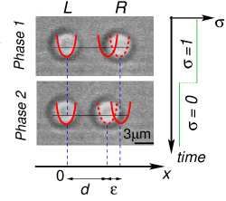
Figure 1: (Color online) The two-bead micropump setup. Bead L is held in a stationary optical trap, while bead R is subject to a time-reversible driving force from a switching optical trap. This assembly is capable of generating flow. The harmonic trap potential is shown schematically overlaid on snapshots taken from the experiments.

The pump is composed of two spheres of radius $a$ labelled with $L$ (Left) and $R$ (Right), positioned on the $x$-axis at an initial distance $d$ as illustrated in FIG. 1. Each sphere is subject to an harmonic potential, which is realized experimentally by an optical trap, anchored to the laboratory reference frame. Bead $R$ is actively driven: its confining potential switches between two positions along the $x$ direction separated by a distance $\varepsilon$, with a frequency $1/2\tau$. The position of the minimum varies as a function of time as a a square wave according to $\sigma(t)=\chi[2n\tau,(2n+1)\tau](t)$, where $\chi$ denotes the indicator function and $n$ is a positive integer. Bead $L$ is in a stationary potential. There are two distinct phases, corresponding to the values $\sigma=1,0$ of the active drive, which constitute a basic cycle of dynamics.

Despite the fact that the trap movement is reciprocal in time, the external actuation by means of springs cannot guarantee an instantaneous balance of the active forces, so the pump is not instantaneously force-free Lauga (2007); Lauga and Powers (2009). Unlike for swimmers, however, this is not problematic: a pump is a spatially confined system and its center of mass lies within a bounded region. In this system this circumstance is also a necessary condition, assuring that two degrees of freedom are accessible for pumping. Notably, a weaker condition holds: the pump is force-free on average over a cycle period.

In a low Reynolds number fluid, the actively driven particle undergoes a purely dissipative dynamics, just like a forced oscillator that relaxes towards the minimum of its confining potential. While bead $R$ moves, it interacts hydrodynamically with bead $L$, which can vary its position thanks to the softness of the harmonic potential. Their dynamics is described, in the regime where $a\ll d$, using the Oseen tensor approximation Doi and Edwards (1986). Denoting with $x_{L}$ the coordinate of $L$ and similarly for $R$, the governing equations read

$$\left\{\begin{array}[]{c}\dot{x}_{L}=-\omega x_{L}-\omega\dfrac{\lambda}{r}\Big{(}x_{R}-(d-\varepsilon\sigma)\Big{)};\\ \\ \dot{x}_{R}=-\omega\Big{(}x_{R}-(d-\varepsilon\sigma)\Big{)}-\omega\dfrac{\lambda}{r}x_{L};\\ \end{array}\right.$$ (1)

where we have introduced the three parameters $\gamma=6\pi\eta a$, $\omega={k}/{\gamma}$, $\lambda={3a}/{2}$ and the relative distance $r=x_{R}-x_{L}$. Here $\eta$ is the fluid viscosity, $\gamma$ is the Stokes’ drag coefficient and $k$ is the stiffness of the spring. The equations show that the geometric parameters of the model have a clear interpretation: the inverse of $d$ sets the strength of the hydrodynamic coupling between the spheres, and $\varepsilon$ is the oscillation amplitude of the actively driven particle.

The model reveals an intriguing property. The presence of two active drives, without any constraint, would provide the system with two “obvious” degrees of freedom. However, the temporal dependence of the active mechanism described here is symmetric under time reversal, as can be seen by inspecting FIG. 1 from top to bottom and vice-versa. Thus, at first sight it might appear that the system cannot generate net flow. Instead, the left-right symmetry is broken.

The pumping can be quantified by focusing on the bead in the resting trap, $L$; an asymmetry in its trajectory reveals an asymmetry in the flow field. We define the order parameter

$$\overline{\Delta x}(d,\varepsilon,\tau):=\dfrac{1}{2\tau}\int^{2\tau}_{0}x_{L}dt$$ (2)

to quantify the magnitude and the direction of the flow as a function of the parameters $d$, $\varepsilon$ and $\tau$. Its physical interpretation is as follows. Imagine that bead $L$ is an isolated sphere attached to a spring, and subject to the same flow field as the one generated by the pump. Then Hooke’s law gives $\overline{F}=k\overline{\Delta x}$, allowing to measure the equivalent mean force exerted by the pump. Using Stokes’ law this flow field can be converted into a mean velocity of the fluid $\overline{v}={\overline{F}}/{\gamma}$.

The analysis of the two phases of motion helps to understand how the symmetry breaking occurs . I) in $Phase\,1$, the hydrodynamic coupling between beads $L$ and $R$ has a strength of the order of ${1}/{d}$ and increases as the spheres approach to reach their minimum distance. According to the positions of bead $L$, the fluid is pushed in the sense $x<0$. Eventually bead $L$ is restored back to equilibrium $x_{L}=0$, and in this relaxation some fluid is dragged in the opposite direction. II) in $Phase\,2$, hydrodynamic coupling is stronger [on the order of ${1}/{(d-\varepsilon)}$]. The dynamics looks similar to the mirror image of the previous one, with bead $R$ dragging bead $L$ in the sense of $x>0$, but now the stronger coupling moves a greater amount of fluid. The overall effect is a net thrust in this direction. An example of such motion for bead $L$ is illustrated in FIG. 3(a). The mismatch in hydrodynamic coupling between end of $Phase\,1$ and beginning of $Phase\,2$ is the root of the symmetry breaking and is made possible by the softness of the driving potentials. Such a phenomenon is analogous to the soft swimming described in Trouilloud et al. (2008). As we see the pumping direction is determined by the position of the actuated particle: if bead $R$ is active, the pumping is in the direction of $x>0$ and vice versa if bead $L$ is active.

Introducing the reduced distance $u=r-d$ and mean coordinate $c=(x_{L}+x_{R})/2$, in the approximation of small oscillations the equations of motion can be expanded as power series in the parameter ${u}/{d}$. With this change, equations (1) decouple into an equation for $u$, independent of $c$, and a linear equation for $c$ involving both variables. The dynamics at the leading order in $u$ is obtained by substituting $1/(u+d)\approx 1/d$ in the resulting equations. This corresponds to the study of the linearized system and a careful analysis shows that no pumping is achieved. Physically, this fact can be understood by interpreting $1/r$ as an effective drag felt by the center of mass $c$. When $r$ is approximatively constant, then the drag doesn’t change during the two phases of dynamics causing therefore no net thrust on $c$ and thus on the fluid.

Pumping arises as a non-linear effect which can be seen already at the next order of expansion. According to $1/(d+u)\approx 1/d-u/d^{2}$, the reduced distance $u$ has to satisfy of a set of Riccati equations depending on the parameter $\sigma$:

$$\dot{u}=\mathcal{P}_{\sigma}+\mathcal{Q}_{\sigma}u+\mathcal{R}u^{2},$$ (3)

where we have defined $\mathcal{P}_{\sigma}:=-\varepsilon\sigma\omega\left(1-\lambda/d\right)$, $\mathcal{Q}_{\sigma}:=-\omega\left(1-\lambda/d+\sigma(\lambda\varepsilon)/d^{2}\right)$ and $\mathcal{R}:=-\omega\lambda/d^{2}$. The center of mass equation maintains its linear character,

$$\dot{\tilde{c}}_{\sigma}=-\omega\left(1+\dfrac{\lambda}{d}-\dfrac{u\lambda}{d^{2}}\right)\tilde{c}_{\sigma}$$ (4)

for the reduced variable $\tilde{c}_{\sigma}:=c-\left(d-\varepsilon\sigma\right)/2$. Both equations can be solved for $\sigma=0,1$. Further one must impose appropriate conditions on the solutions, representing: (i) the continuity of the whole solution in the middle of the cycle where $u_{0}(\tau)=u_{1}(\tau)$ and $c_{0}(\tau)=c_{1}(\tau)$; and (ii) the steady state condition for which the positions at the beginning of the cycle coincide with those at the end, given by $u_{0}(2\tau)=u_{1}(0)$ and $c_{0}(2\tau)=c_{1}(0)$. Finally, using the inverse transformation from $u,c$ to get $x_{L}$ and $x_{R}$ and taking the temporal average of $x_{L}$, we find that the order parameter $\overline{\Delta x}$ shows a net pumping over two phases of dynamics.

FIG. 2 reports the plots of the resulting expression as functions of $\varepsilon$, $\tau$, $d$ for typical experimental values of $a$ and $\omega$. There, the geometrical variables $\varepsilon$ and $d$ follow the straightforward trend where larger oscillation amplitudes $\varepsilon$ generate larger flow. Also, larger distance $d$ is related to smaller generated flow. However, the plots show also a non-trivial behavior as a function of the temporal parameter $\tau$. The form of the solution suggests a natural way to rescale the parameters, defining the nondimensional quantities $\varepsilon^{*}:=\varepsilon/a$, $d^{*}:=d/a$ and $\tau^{*}:=\tau\omega$. There are two different regimes, i) for small values of $\tau^{*}$ the flow increases and ii) for large values of $\tau^{*}$ it decreases. The reason for the latter is that in this regime the beads have sufficient time to relax in the harmonic traps, so that the area described by the function $x_{L}$ reaches a maximum value, after which it remains constant at increasing $\tau^{*}$. Dividing this area by $\tau^{*}$ gives a decreasing function of $\tau^{*}$. Interestingly, at the intersection of these two regimes the plot shows that $\overline{\Delta x}$ presents a maximum, thus defining an optimal pumping region. Due to the particular form of the function $\overline{\Delta x}$, however, this has to be evaluated numerically. For the typical experimental values in use it corresponds to $\tau\approx 165$ms.

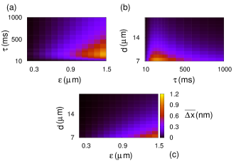
Figure 2: (Color online) Analytical characterization of the pump. (a) $\overline{\Delta x}$ as function of $\varepsilon$ and $\tau$. The trend as a function of $\varepsilon$ is intuitive: the larger the oscillation amplitude, the larger the generated flow. There is a non trivial behavior as function of $\tau$, showing that the maximum pumping is obtained at maximum $\varepsilon$ for some value of $\tau$ in the middle of the scale. $d$ here is fixed to the experimental value of $6\mu$m. (b) $\overline{\Delta x}$ as function of $d$ and $\tau$. We see the same phenomenology as in (a). Here the effect of the distance is to decrease the pumping monotonically. (c) Plot of $\overline{\Delta x}$ as a function of $\varepsilon$ and $d$. Again, it shows a monotonic dependence from the distance and $\varepsilon$. Looking at these plots, is easy to understand that the scaling exponents of $\overline{\Delta x}$ are functions of all these parameters. In particular, the scaling law of $\overline{\Delta x}$ with $\varepsilon$ depends on $\tau$. In all these cases the values of $\omega$ and $a$ are set to typical values taken from the experiments.

For $\tau\gg 1/\omega$, where we can compare with our experimental data, the expression of $\overline{\Delta x}$ simplifies considerably. At the leading order the result is a simple power law dependence

$$\dfrac{\overline{\Delta x}}{a}\approx\dfrac{9}{16\tau^{*}}\dfrac{(\varepsilon^{*})^{2}}{(d^{*})^{3}}.$$ (5)

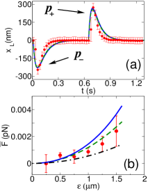
Figure 3: (Color online) Experiment, analytical calculations and simulations agree in quantifying flow generation by the two-bead micropump. (a) As bead R is driven by the optical trap, it causes displacements of bead $L$ around its equilibrium position. Markers show the position of bead L averaged over many cycles. The analytical solution, (green dashed curve) and simulation data (blue continue curve) closely reproduce the experiments. The displacement values $p_{+}$ and $p_{-}$ at the peaks are an accurately measurable quantity. Matching the simulations to the peak values enables the observed $p_{+}$ and $p_{-}$ to be converted to force by a one-to-one mapping; (b) The mean force exerted by the pump on the fluid is measured from the motion of the bead in the stationary trap, and it grows as a function of the pump stroke length $\varepsilon$. Markers and lines are as in panel (a). In addition the approximate solution, Eq. (5) is shown (black dash dotted line).

Integration of the full equations of motion (1) is also performed numerically by means of Taylor’s method Lagomarsino et al. (2003). Comparison with the analytical results shows a good agreement, despite the low-order expansion of the analytical solution, as can be seen by looking at FIG. 3(a),(b). This is not surprising as the Oseen tensor is a description valid for of large separation of the beads, and in this regime the perturbative result is a good approximation to the exact solution.

The dynamics has been investigated experimentally by means of an optical tweezer, described fully in Leoni et al. (2009). A laser beam (IPG Photonics, PYL-1-1064-LP, $\lambda$ = 1064nm, Pmax = 1.1W) is focused through a water immersion objective (Zeiss, Achroplan IR 63x/0.90 W), trapping from below. The laser beam is steered via a pair of acousto-optic deflectors (AA Opto-Electronic, AA.DTS.XY-250@1064nm) controlled by custom built electronics, allowing multiple trap generation by time sharing, with sub-nanometer position resolution. Instrument control and data acquisition (70 frames per second, with an exposure time of 13 ms) are performed by custom software.

A typical experiment consists of trapping two silica beads (3.0$\mu$m diameter, Bangs Labs) in a solution of glycerol (Fisher, Analysis Grade) and is divided in two parts: in the first calibration stage all the traps are kept at rest, and the beads undergo only Brownian motion confined by the traps. During the second stage we reproduce the cycle of FIG. 1 with lasers traps, iterating the sequence many times Leoni et al. (2009). The whole procedure lasts typically 6 minutes, during which we collect about 40 000 frames. We performed 3 runs for each set of parameters.

By analyzing images by correlation filtering and two dimensional fitting, we obtain the beads’ position with subpixel (around 1nm) resolution. The expected values of $\overline{\Delta x}$ are below the limit of the experimental resolution (indeed the smallest forces measured here correspond to 0.1nm displacements), and therefore we characterize the pumping indirectly, relying on the measurable asymmetry of peaks of bead $L$’s position Leoni et al. (2009). Regarding each cycle as an independent realization of a stochastic process, we construct the mean dynamic cycle of $L$, see FIG. 3(a). Compared to the equilibrium position of the bead, that can be determined from the mean cycle itself but only for large values of $\tau^{*}$ when the dynamics is fully relaxed, we indicate the maximum with $p_{+}$ and the minimum with $p_{-}$. We define the algebraic sum $\delta:=p_{+}+p_{-}$ to quantify the asymmetry of motion and convert it to $\overline{\Delta x}$ with the aid of simulations. This procedure allows to compare extremely small forces, of the order of $5\times 10^{-4}$pN, which, to our knowledge, are the smallest forces measured with optical traps.

In FIG. 3(b) we plot the corresponding mean force obtained from the experiments at varying $\varepsilon$ and compare this result with analytical predictions and simulations. The experimental values considered are $a=1.5\mu$m, $d=6\mu$m, $\tau=640$ ms, $\omega=0.022\pm 0.001(\mathrm{ms})^{-1}$, $T=25^{o}$ C and a trap stiffness value of $k=5.32\pm 0.71$ pN/$\mu$m. The results show a good agreement between the measured force and the predicted values. Approximate analytical solution (5) gives a good description of pumping.

It is interesting to compare the effectiveness of the current minimal pump to the related three-bead model system Leoni et al. (2009). Close to the optimal pumping region, and for matching values of the stroke $\epsilon$ and inter-particle distance $d$, the average force exerted on the fluid by the three-bead model exceeds the two-bead companion by about one order of magnitude. The poorer performance with two beads is not surprising, and minimality is obtained at the expense of performance. However we would like to point out that the two pumps have also a profoundly different nature. In the three-bead model, pumping is achieved by moving the lateral beads in a non-reciprocal fashion. The direction of the flow is determined by the first moving trap and can be reverted inverting the trap moves. The nature of the drive in the two-bead model prevents all this and the pumping direction is uniquely determined by the disposition of the active trap, as discussed above.

In conclusion, an extremely simple system composed of just two spherical beads, only one of which is actuated by a time-reversible trap movement, is shown to be capable of generating flow. A key property of the system is that the beads are held and driven by soft potentials. This allows the two-bead system to explore two degrees of freedom, thus satisfying the “scallop theorem”. The simplicity of this elementary pump makes it possible to understand the fluid dynamics analytically, and suggests this as a feasible micro-pump that could be deployed experimentally in the context of microfluidic systems.