Cusps in interfacial problems

Abstract

A wide range of equations related to free surface motion in two dimensions exhibit the formation of cusp singularities either in time, or as function of a parameter. We review a number of specific examples, relating in particular to fluid flow and to wave motion, and show that they exhibit one of two types of singularity: cusp or swallowtail. This results in a universal scaling form of the singularity, and permits a tentative classification.

I Introduction

The geometry of singularities of wavefronts, i.e. caustics, has been much studied Nye (1999). The caustics, themselves, exhibit singularities such as cusps, which can be classified using catastrophe theory Arnold (1984); Poston and Stewart (1978). In the present review we point out that a similar classification appears to apply in a variety of nonlinear PDE problems, which describe the motion of a free (fluid) surface.

The two-dimensional problems studied here can be written as a mapping of the physical domain to the unit disc, the free surface being represented as the circle. The appearance of a singularity is associated with the non-invertibility of this conformal map at a given value of time or of some other parameter. Since the problems studied here are endowed with a holomorphic structure, such non-invertibility has a very particular geometrical consequence: the formation of a cusp with a 2/3 exponent or of a swallowtail singularity. When looking at the mapping as it evolves in time, or depends on a parameter, it is apparent that the mapping remains smooth as the self-intersection occurs. For this reason the curve can be written as an analytic function of a suitable parameter. Performing a local expansion around the point of self-intersection, the properties of the curve are determined by the lowest order terms of the Taylor expansion in the parameter.

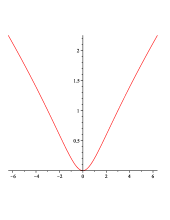
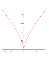
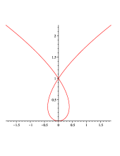
Figure 1: The formation of a cusp, as described by (1). Shown is a non-intersecting curve ($\epsilon=2$), a 2/3 cusp ($\epsilon=0$), and a loop ($\epsilon=-1$), from left to right.

The simplest case of self-intersection is that of the cusp. Let us assume that the coordinates $x$ and $y$ can be expanded into a Taylor series as function of some parameter, $\theta$, and that we are interested in the neighborhood of $\theta=0$. Since we describe phenomena up to arbitrary translations, the generic description is $x=a_{1}\theta$ and $y=a_{2}\theta$. However, by performing a rotation one can always make sure that one of the coefficients ($a_{2}$, say), is zero. The singular case corresponds to the situation where $a_{1}$ vanishes as well, so we put $x=\epsilon\theta$, with the singularity at $\epsilon=0$.

Of course we are now required to expand to higher order. The next non-trivial order in $y$ gives $y=\theta^{2}/2$, where the coefficient can be normalized by rescaling $\theta$. The expansion in $x$ has to be pursued to third order, otherwise the curve would be degenerate for $\epsilon=0$. Thus we finally have:

$$x=\epsilon\theta+a\theta^{3}/3,\quad y=\theta^{2}/2,$$ (1)

where $a$ is an arbitrary constant. The quadratic coefficient in the expansion of $x$ can be eliminated by a shift in $\theta$, with subsequent rotation and translation. Thus up to translations and rotations, (1) is the only generic way the self-intersection of a curve in the plane can occur, as illustrated in Fig. 1. For $\epsilon<0$ the curve self-intersects, at the critical point $\epsilon=0$ a cusp is formed. It is clear from (1) that this cusp has the form $y=(x/a)^{2/3}$, i.e. it is associated with a universal power law exponent. In catastrophe theory Arnold (1984), (1) is the curve associated with the “cusp” catastrophe.

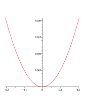
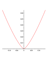
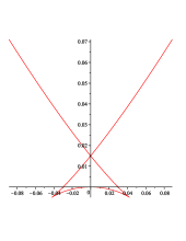
Figure 2: The formation of a swallowtail, as described by (3). Shown is a smooth minimum, ($\epsilon=1$, left), a minimum with a 4/3 singularity ($\epsilon=0$, right), and a swallowtail or double cusp ($\epsilon=-1/2$, right).

As we will see below, higher order singularities can also occur, which presumably is due to a hidden symmetry of the problem. As a result, the coefficient in front of the quadratic term vanishes in (1): $y=\epsilon_{s}\theta^{2}/2+b_{1}\theta^{3}/3+b_{2}\theta^{4}/4$. Once more, the cubic term can be made to vanish by performing a rotation, so we arrive at the following generic form:

$$x=\epsilon_{s}\theta+a\theta^{3}/3,\quad y=\epsilon_{s}\theta^{2}/2+b\theta^{4}/4,$$ (2)

which exhibits a much milder singularity. Namely, for $\epsilon_{s}=0$ the behavior is like $y\propto x^{4/3}$. For $\epsilon_{s}<0$, the curve splits into two cusp singularities of the form shown in Fig. 1, where the case $b>a$ corresponds to $\epsilon>0$ in the representation (1), $b<a$ to $\epsilon<0$. In all the cases to be discussed below, we always find the particular case $a=b$, which means for $\epsilon_{s}<0$ the solution is exactly at the cusp singularity. This is the swallowtail known from catastrophe theory, which can be seen as a collision of two cusps (see Fig. 2). It has the universal form

$$x=\epsilon\theta+a\theta^{3}/3,\quad y=\epsilon\theta^{2}/2+a\theta^{4}/4,$$ (3)

once more with $\epsilon,a$ being parameters.

The two catastrophes (1) and (3) can occur either as function of time or of some control parameter. Let us introduce the time distance $t^{\prime}=t_{0}-t$ to the singularity, and assume the scaling $|\epsilon|=|t^{\prime}|^{\gamma}$. The time before the singularity $t^{\prime}>0$ corresponds to $\epsilon>0$, and vice versa. Then

$$x=|t^{\prime}|^{3\gamma/2}X_{c},\quad y=|t^{\prime}|^{\gamma}Y_{c},$$ (4)

$$X_{c}=\pm\sigma+a\sigma^{3}/3,\quad Y_{c}=\sigma^{2}/2,$$ (5)

is the self-similar form of the cusp singularity, and

$$x=|t^{\prime}|^{3\gamma/2}X_{s},\quad y=|t^{\prime}|^{2\gamma}Y_{s},$$ (6)

$$X_{s}=\pm\sigma+a\sigma^{3}/3,\quad Y_{s}=\pm\sigma^{2}/2+a\sigma^{4}/4$$ (7)

of the swallowtail singularity. In each case, the + or - signs correspond to the similarity function before or after the singularity, respectively. We remark that the cusp singularity can be written as the following cubic:

$$X_{c}^{2}=2Y_{c}(1\pm 2aY_{c}/3)^{2}.$$ (8)

As we have mentioned before, the similarity function (6) valid after the singularity contains two cusp singularities, which occur for $\sigma=\pm 1/\sqrt{a}$. Thus if one writes $\sigma=\pm 1/\sqrt{a}+s$, shifts the cusp to the origin and performs a rotation, one obtains to leading order in $s$:

$$\left(\begin{array}[]{c}\pm as^{3}\\ (a+1)s^{2}\end{array}\right)=\left(\begin{array}[]{cc}1&\mp\sqrt{a}\\ \pm\sqrt{a}&1\end{array}\right)\left(\begin{array}[]{c}X_{s}\pm 2/(3\sqrt{a})\\ Y_{s}+1/(4a)\end{array}\right)$$ (9)

The + or - signs correspond the left and right cusp, respectively. This demonstrates that $(X_{s},Y_{s})$ locally traces out a cusp after the swallowtail singularity, as seen in Fig. 2.

Equation	Type	$\gamma$	Section
Wave fronts	swallowtail	1	II
Hele-Shaw flow	cusp	1/2	III
Potential flow with free surface	swallowtail	//	IV
Porous medium equation	cusp	//	V
Viscous flow with free surface	cusp	//	VI
Born Infeld equation	swallowtail	1	VII

Table 1: A summary of evolution equations discussed in this paper. The classification as “cusp” or “swallowtail” refers to (1) or (3), respectively. In the case of time-dependent problems, the exponent $\gamma$ is defined by (4) or (6), depending on the type of singularity.

Table 1 summarizes the the problems to be studied in this paper, and cites the relevant sections. Each equation, to be discussed in more detail in the sections below, exhibits singularities which can be classified as either being of the “cusp” or the “swallowtail” type. Some are evolution equations, in which case we give the temporal scaling exponent $\gamma$, others exhibit singularities as function of a parameter. In each case, we attempt to give physically motivated examples.

II The eikonal equation

II.1 Hamilton-Jacobi equation

We consider the simplest case of wave propagation in a homogeneous medium, so the eikonal equation becomes $V_{n}=1$: the normal velocity of the wave front is constant everywhere. We will only consider wave propagation in two dimensions, so the wave front is a curve. A straightforward way to solve the eikonal equation is to consider $y=h(x,t)$ so that one can write the equation in the form

$$h_{t}=\sqrt{1+h_{x}^{2}},\quad h(x,0)=h_{0}(x),$$ (10)

which expresses the condition of constant normal velocity.

To solve (10), we pass to the “particle” description; the equation for the wave front (10) is the Hamilton-Jacobi equation for the Hamiltonian

$$H(x,p)=-\sqrt{1+p^{2}},$$ (11)

where $p=h_{x}$. The initial condition $(x_{0},h_{0}^{\prime}(x_{0}))$ yields a curve $(x,p)$ in phase space, and the trajectories will be

$$\frac{dx}{dt}=\frac{\partial H}{\partial p}=-\frac{p}{\sqrt{1+p^{2}}},\quad\frac{dp}{dt}=-\frac{\partial H}{\partial x}=0.$$ (12)

Thus the solution to the particle problem is

$$p=const=h_{0}^{\prime}(x_{0}),\quad x=x_{0}-\frac{p}{\sqrt{1+p^{2}}}t=x_{0}-\frac{h_{0}^{\prime}(x_{0})}{\sqrt{1+h_{0}^{\prime 2}(x_{0})}}t.$$ (13)

We can obtain an explicit solution by noting that

$$\frac{dh}{dx}=\frac{dh}{dx_{0}}\frac{dx_{0}}{dx}=h_{0}^{\prime}(x_{0}),$$

where from (13)

$$\frac{dx}{dx_{0}}=1-\frac{h_{0}^{\prime\prime}}{\sqrt{1+h_{0}^{3}}}t.$$

Integrating the resulting expression for $dh/dx_{0}$, we finally obtain

$$x=x_{0}-\frac{h_{0}^{\prime}}{\sqrt{1+h_{0}^{\prime 2}}}t,\quad h=h_{0}(x_{0})+\frac{t}{\sqrt{1+h_{0}^{\prime 2}}}.$$ (14)

This is an explicit solution of (10), which has the additional advantage that it can be continued across any singularity the wave front may encounter.

A caustic is a place where rays meet, and thus $dx/dx_{0}=0$, $dy/dx_{0}=0$. The two conditions turn out to be equivalent, and one obtains

$$t_{c}=\frac{\sqrt{1+h_{0}^{\prime 2}}^{3}}{h_{0}^{\prime\prime}}\equiv 1/\kappa.$$ (15)

It is also clear that points on the caustic correspond to singularities of the wave front Berry (1992). The first singularity occurs at a time $t_{0}$ corresponding to the maximum of the curvature, for which there is optimal focusing. The universal structure is obtained by expanding $h_{0}$ in a series, which without loss of generality only contains even terms:

$$h_{0}=a_{1}x_{0}^{2}+a_{2}x_{0}^{4}+\dots.$$ (16)

The first singularity occurs for $t_{0}=1/(2a_{1})+\dots$, and an expansion leads precisely to (6), namely

$$x=t^{\prime}\sigma+a\sigma^{3}/3$$ (17)

$$y=1/(2a_{1})-t^{\prime}+t^{\prime}\sigma^{2}/2+a\sigma^{4}/4,$$

where $a=3(a_{1}^{3}-a_{2})/(4a_{1}^{4})$, and $\sigma=2a_{1}x_{0}$; the scaling exponent is $\gamma=1$. After the singularity, $t^{\prime}<0$, (17) is a swallowtail, and the two cusp points trace out the caustic. This corresponds to the positions $\sigma_{c}=\pm\sqrt{-t^{\prime}/a}$, and so to leading order the equation of the caustic is

$$x_{c}=\pm\frac{-4t^{\prime 3/2}}{a^{1/2}},\quad y_{c}=\frac{1}{2a_{1}}-t^{\prime},$$ (18)

which is a normal 2/3-cusp, see Fig. 3.

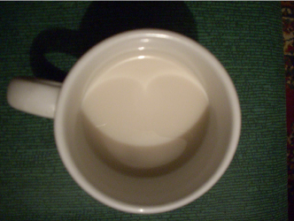
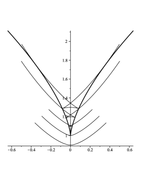
Figure 3: A caustic in a coffee cup. On the left, physical reality. On the right, the evolution of the wave front, as it passes through the swallowtail singularity. The caustic forms a 2/3-cusp, which corresponds to a swallowtail in terms of the shape of the wavefront.

II.2 conformal mapping

There is a second way of solving the eikonal equation, closer to the methods to be used in the next sections, based in the use of a complex representation of the front. We present it here to stress the similarities between the different problems studied in this paper. If one identifies the points of the curve $(x(\sigma,t),y(\sigma,t))$ as points $z(\sigma,t)=x(\sigma,t)+$ $iy(\sigma,t)$ in the complex plane, and the velocity $\mathbf{u}=(u,v)$ as the complex number $u+iv$, then

$$z_{t}=u+iv.$$ (19)

The tangent and normal vectors have a complex representation

$$\mathbf{t}=z_{s},\quad\mathbf{n}=iz_{s},$$ (20)

where $s$ is the arclength parameter. Hence we can write

$$\mathbf{u}\cdot\mathbf{n}=\mathrm{Re}\left(iz_{s}\overline{z_{t}}\right)=-\mathrm{Im}\left(z_{s}\overline{z_{t}}\right),$$

and the eikonal equation is simply

$$\mathrm{Im}\left(z_{s}\overline{z_{t}}\right)=-1,$$ (21)

with the constraint $|z_{s}|=1$. Equivalently, one can introduce an arbitrary parameter $\sigma$ of the curve, and (21) becomes or, equivalently,

$$\mathrm{Im}\left(z_{\sigma}\overline{z_{t}}\right)=-\frac{ds}{d\sigma},$$ (22)

without the necessity of introducing a constraint.

We now demonstrate that (22) yields the same local solution as before, by verifying that (17) yields, at leading order, a solution of (22):

$$z_{\sigma} = (t^{\prime}+a\sigma^{2})+i(t^{\prime}\sigma+a\sigma^{3})\ ,\ z_{t}=-\sigma+i(1-\sigma^{2}/2)$$

$$\mathrm{Im}\left(z_{\sigma}\overline{z_{t}}\right) = -(1+\frac{\sigma^{2}}{2})(t^{\prime}+a\sigma^{2})$$

$$\frac{ds}{d\sigma} = \sqrt{(t^{\prime}+a\sigma^{2})^{2}+\sigma^{2}(t^{\prime}+a\sigma^{2})^{2}}=(1+\frac{\sigma^{2}}{2})(t^{\prime}+a\sigma^{2}+O(\sigma^{4})).$$

III Hele-Shaw flow

A Hele-Shaw cell consists of two closely spaced glass plates, partially filled with a viscous fluid. The problem is to find the time evolution of the free interface between fluid and gas. Here we consider the case that the fluid occupies a closed two-dimensional domain $\Omega$. Within $\Omega$, the pressure obeys $\Delta p=0$, with boundary conditions

$$p = 0$$ (23)

$$V_{n} = -\nabla p\cdot\mathbf{n}$$ (24)

on the free surface $\partial\Omega$. We write $z=x+yi$ and

$$p=\rm{Re}\Phi(z)$$

together with the conformal mapping

$$z=f(\xi,t),\quad\xi=re^{i\theta},$$ (25)

which maps $\left|\xi\right|=1$ onto $\partial\Omega$. If we consider

$$\Phi(z(\xi,t))=\log\xi\ \ \ \text{inside }\Omega,$$

then condition (23) is automatically satisfied. Moreover

$$-\nabla p\cdot\mathbf{n}=-\rm{Re}\left(\frac{\partial\Phi}{\partial z}iz_{s}\right)=-\rm{Re}\left(\frac{\partial\Phi}{\partial\xi}\frac{1}{z_{\xi}}iz_{s}\right)=-\rm{Re}\left(\frac{1}{\xi z_{\xi}}iz_{s}\right),$$

where $s$ is the arclength parameter. Notice that one can write for $\left|\xi\right|=1$, using $\xi=e^{i\theta(s,t)}$

$$z_{s}=z_{\xi}\xi_{s}=z_{\xi}\xi i\theta_{s},$$

and hence

$$-\nabla p\cdot\mathbf{n=}\theta_{s}.$$ (26)

Since

$$V_{n}=\rm{Re}\left(\overline{z_{t}}iz_{s}\right)=-\theta_{s}\rm{Re}\left(\overline{z_{t}}\xi z_{\xi}\right)$$

we arrive, combining this with (26), at the equation

$$\rm{Re}\left(\overline{z_{t}}\xi z_{\xi}\right)=-1.$$ (27)

Noting that $\xi z_{\xi}=\frac{1}{i}z_{\theta}$, we finally obtain

$$\rm{Im}\left(z_{\theta}\overline{z_{t}}\right)=-1.$$ (28)

Equation (28) is identical to (21) except for the fact that the space variable is not the arclength parameter $s$, but the an arbitrary parameter $\theta$. The non-invertibility of $f(\xi,t)$ signals the appearance of a singularity.

Now we will present an exact solution of (27), using a particular (polynomial) ansatz for the mapping 25 Polubarinova-Kochina (1945a, b); Galin (1945); Howison (1986). We consider the simplest case of a quadratic:

$$f(\xi,t)=a_{1}(t)\xi+a_{2}(t)\xi^{2},$$ (29)

and show that it leads to cusped solutions. However, we expect cusp formation to be a generic feature. The reason is that the formation of a singularity is associated to the non-invertibility of the conformal map $f(\xi,t)$ and this is equivalent to $f^{\prime}(\xi,t)$ being zero at some point $\xi_{0}$ (at the time $t_{0}$ of formation of the singularity), which leads to a generic quadratic behavior of $f(\xi,t_{0})=b_{0}+b_{2}(\xi-\xi_{0})^{2}$ near $\xi_{0}$. Other local expansions of $f(\xi,t_{0})$ around $\xi_{0}$, of the form $f(\xi,t_{0})=b_{0}+b_{n}(\xi-\xi_{0})^{n}$ with $n>2$ are also possible. They would lead to different form of cusp, but cannot be generic since small perturbations of the initial data would produce quadratic terms.

Inserting (25),(29) into (28), we find a solution if the following system of ODEs is verified:

$$a_{1}a_{1}^{\prime}+2a_{2}a_{2}^{\prime}=-1$$ (30)

$$a_{1}a_{2}^{\prime}+2a_{2}a_{1}^{\prime}=0.$$ (31)

Direct integration of the equations leads to

$$\frac{1}{2}a_{1}^{2}+\frac{B^{2}}{a_{1}^{4}}=A-t$$ (32)

$$A=\frac{1}{2}a_{1}^{2}(0)+a_{2}^{2}(0)\ ,\ B=a_{2}(0)a_{1}^{2}(0)$$ (33)

A singularity occurs when $f$ fails to be invertible, that is

$$\frac{df}{d\xi}=a_{1}+2a_{2}\xi=0\Rightarrow\xi=-\frac{a_{1}}{2a_{2}}=-1$$ (34)

or equivalently when

$$a_{1}-4\frac{B^{2}}{a_{1}^{5}}=0\Rightarrow a_{1}=(2B)^{\frac{1}{3}},a_{2}=\frac{1}{2}(2B)^{\frac{1}{3}}.$$ (35)

From (32) one can compute the singularity time

$$t_{0}=A-\frac{3}{4}(2B)^{\frac{2}{3}}=\frac{1}{2}a_{1}^{2}(0)+a_{2}^{2}(0)-\frac{3}{4}(2a_{2}(0)a_{1}^{2}(0))^{\frac{2}{3}}.$$

Now let us consider a particular solution, for instance

$$a_{1}(0)=1\ ,\ a_{2}(0)=\frac{1}{16},$$ (36)

so that

$$A=\frac{129}{256},B=\frac{1}{16},\ t_{0}=\left(\frac{3}{4}\right)^{4}\ ,\ a_{1}(t_{0})=\frac{1}{2}\ ,a_{2}(t_{0})=\frac{1}{4}.$$

This implies the formation of a singularity at $x(\pi,t_{0})=-\frac{1}{4}$ and $y(\pi,t_{0})=0$.

Local analysis leads to $a_{1}(t)=1/2+\widetilde{a}(t)$, where $3\widetilde{a}^{2}(t)\sim t_{0}-t$. Thus the scale factor $\widetilde{a}(t)$ is

$$\widetilde{a}(t)\sim\frac{1}{\sqrt{3}}(t_{0}-t)^{\frac{1}{2}}\equiv\frac{1}{\sqrt{3}}t^{\prime\frac{1}{2}}.$$ (37)

and $a_{2}(t)=1/(16a_{1}^{2}(t))\sim 1/4-\widetilde{a}(t)$. Writing $\xi=-1+\widetilde{\xi}$, we deduce

$$f(\xi,t)=a_{1}(t)\xi+a_{2}(t)\xi^{2}\sim-1-2\widetilde{a}(t)+3\widetilde{a}(t)\widetilde{\xi}+\frac{1}{4}\widetilde{\xi}^{2}.$$ (38)

Since

$$-1+\widetilde{\xi}=-e^{i(\theta-\pi)}=-1+(1-e^{i\widetilde{\theta}})\simeq-1+\frac{\widetilde{\theta}^{2}}{2}-\frac{\widetilde{\theta}^{4}}{4!}-i\widetilde{\theta}+i\frac{\widetilde{\theta}^{3}}{3!}+O(\widetilde{\theta}^{5})$$

one has

$$f(\xi,t)\sim-1-2\widetilde{a}(t)+3\widetilde{a}(t)\left(\frac{\widetilde{\theta}^{2}}{2}-\frac{\widetilde{\theta}^{4}}{4!}-i\widetilde{\theta}+i\frac{\widetilde{\theta}^{3}}{3!}\right)-\frac{1}{4}\widetilde{\theta}^{2}+\frac{1}{16}\widetilde{\theta}^{4}-\frac{1}{4}\widetilde{\theta}^{3}i+O(\widetilde{\theta}^{5}),$$

leading to the leading order contributions (all other terms are subdominant for small values of $\widetilde{a}(t)$ and $\widetilde{\theta})$:

$$x(\theta,t)+1 \sim -2\widetilde{a}(t)-\frac{1}{4}\widetilde{\theta}^{2}$$ (39)

$$y(\theta,t) \sim -3\widetilde{a}(t)\widetilde{\theta}-\frac{1}{4}\widetilde{\theta}^{3},$$ (40)

which is the desired local solution we have been looking for.

Defining

$$X_{c}=-\frac{y}{6t^{\prime 3/4}},\ Y_{c}=-\frac{x+1}{6t^{\prime 1/2}}-\frac{1}{3\sqrt{3}},\ \Theta=\frac{\widetilde{\theta}}{2\sqrt{3}t^{\prime 1/4}},$$ (41)

one obtains the cusp (4), with $a=9\sqrt{3}$ and the scaling exponent $\gamma=1/2$. A different choice of initial conditions (36) will of course lead to a different value of the parameter $a$. In Figure 4 we represent the interface profiles corresponding to the example developed above at the initial time and at the time of formation of the cusp.

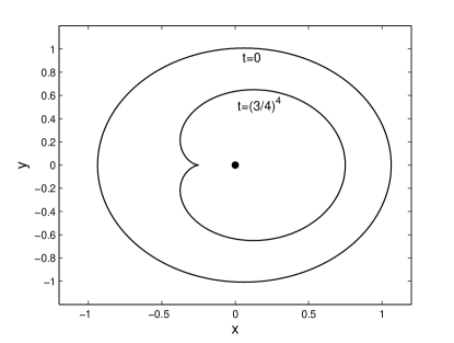
Figure 4: The formation of a cusp in Hele-Shaw problem with suction at the origin.

IV Potential flow

We consider the two-dimensional flow of an ideal fluid below a free surface. Inside the fluid, the fluid velocity ${\bf u}=(u,v)$ satisfies

$${\bf u}=\nabla\phi,\quad\triangle\phi=0,$$ (42)

where $\phi$ is the velocity potential. The free surface is convected by the fluid velocity, and the free surface is at constant pressure. We consider the simplest case of steady flow, as well as no body or surface tension forces. According to Bernoulli’s equation, the fluid speed then has to be constant on the free surface.

Exact solutions to the flow problem can be found if the fluid domain is bounded by free surfaces and straight solid boundaries alone Batchelor (1967), by mapping the fluid domain onto the upper half of the complex plane, which we denote by $\zeta$. Here, we consider only the even simpler case of only free boundaries, i.e. that of a two-dimensional fluid drop. To this end, one introduces the complex potential $w=\phi+i\psi$, where $\psi$ is the stream function. The derivative of $w$ gives the fluid velocity:

$$\frac{dw}{dz}=u-iv\equiv qe^{-i\theta},$$ (43)

where $q$ is the particle speed.

On the fluid boundary, $\psi$ is constant, and this constant can be chosen to vanish. Thus $w(\zeta)$ is real on the real axis (the boundary of the fluid drop), and so $dw/d\zeta$ must be real as well.

Following Hopkinson Hopkinson (1898) we drive a fluid motion inside the drop by placing singularities inside the drop. We will consider the case of a vortex dipole and a vortex at the same point. We have

$$\frac{dw}{d\zeta}=\frac{dw}{dz}\frac{dz}{d\zeta},$$ (44)

where $dz/d\zeta$ contains no singularities in the upper $\zeta$ plane, since the representation of the fluid flow must be conformal. But this means that $dw/d\zeta$ must have the same singularities as $dw/dz$, except that we now have the freedom to choose the position of the two singularities and the orientation of the vortex doublet arbitrarily. Thus if we choose the two singularities at $\zeta=i$, and the orientation of the doublet toward the positive real axis, the potential for the doublet must locally look like $w\propto 1/(\zeta-i)-im\ln(\zeta-i)$. Here $m$ is the relative strength of the vortex.

To insure that $dw/d\zeta$ also obeys the boundary condition, one has to add image singularities at $\zeta=-i$:

$$\frac{dw}{d\zeta}=\frac{1}{(\zeta-i)^{2}}+\frac{1}{(\zeta+i)^{2}}-im\left(\frac{1}{\zeta-i}-\frac{1}{\zeta+i}\right).$$ (45)

Depending on the value of $m$, two different cases arise. For simplicity, we only consider the case $m<1$, in which

$$\frac{dw}{d\zeta}=\frac{2(1+m)(\zeta^{2}-\gamma^{2})}{(\zeta^{2}+1)^{2}},$$ (46)

Where $\gamma=\sqrt{(1-m)/(1+m)}$ real.

Manifestly, $dw/d\zeta$ is real on the real axis, and has the right singularities at $\zeta=i$. However, the information contained in (45) is not enough to reconstruct the mapping $z(\zeta)$ we are after. Following Kirchhoff Kirchhoff (1869) and Planck Planck (1884), we define another function

$$\Omega=\ln\frac{dz}{dw}\equiv-\ln q+i\theta,$$ (47)

which will also be represented in the $\zeta$-plane. Since $q$ is constant along the free surface, and choosing units such that $q=1$, the function $\Omega$ will be purely imaginary on the real $\zeta$ axis. To find $\Omega$, we once more proceed in two steps.

First, we find the singularities of $\Omega$. From the definition,

$$\Omega=-\ln\frac{dw}{d\zeta}+\ln\frac{dz}{d\zeta},$$ (48)

where the second contribution is conformal in the upper half plane. This means $\Omega$ has singularities only for $\zeta=i$, where it behaves like $\Omega\propto 2\ln(u-i)$. Second, we have to make sure that $\Omega$ is imaginary for real $\zeta$, which is achieved by

$$\Omega=2\ln\frac{\zeta-i}{\zeta+i}.$$ (49)

Now we use the fact that

$$\frac{dz}{d\zeta}=\frac{dz}{dw}\frac{dw}{d\zeta}=e^{\Omega}\frac{dw}{d\zeta}=\frac{2(1+m)(\zeta^{2}-\gamma^{2})}{(\zeta+i)^{4}}.$$ (50)

This expression can be integrated to find the transformation $z(\zeta)$ between the fluid domain and the $\zeta$-plane:

$$\frac{z}{2(1+m)}=-\frac{1}{\zeta+i}+\frac{i}{(\zeta+i)^{2}}+\frac{1+\gamma^{2}}{3(\zeta+i)^{3}}.$$ (51)

From the real and imaginary part of this expression, we obtain

$$x=-(2(1+m))\zeta\frac{3\zeta^{4}-(1+\gamma^{2})\zeta^{2}+3\gamma^{2}}{3(\zeta^{2}+1)^{3}}$$ (52)

$$y=(2(1+m))\frac{6\zeta^{4}+3(1-\gamma^{2})\zeta^{2}+1+\gamma^{2}}{3(\zeta^{2}+1)^{3}}.$$ (53)

The mapping is such that $\zeta=\pm\infty$ gets mapped to the origin. A typical drop shape, for $m=1/3$, is shown in Fig. 5 (left); it exhibits two cusps. This feature is generic, in that it exists for a continuous range of values $0.9427\geq m\geq 0$. On the right of show a closeup of the top of the drop, close to the upper end of his range.

The origin of the double cusp lies in a swallowtail transition for $m\approx 1$ that occurs at the point $x=0$, $y=4/3$ in real space. Namely, a local expansion of (53) gives with $m=1+\epsilon$

$$x=2\epsilon\zeta+4\zeta^{3}/3$$ (54)

$$y=4\epsilon\zeta^{2}+4\zeta^{4},$$ (55)

where $\zeta$ is taken as real. The same expression results if the shape of the drop valid for $m>1$ is expanded locally. The corresponding swallowtail is shown in Fig. 6 using the full solution Fig. 53. For $m$ very close to the transition, the free surface must self-intersect, as shown in Fig. 6 (right). However, below a value of about $m\approx 0.9427$ the self-intersection disappears.

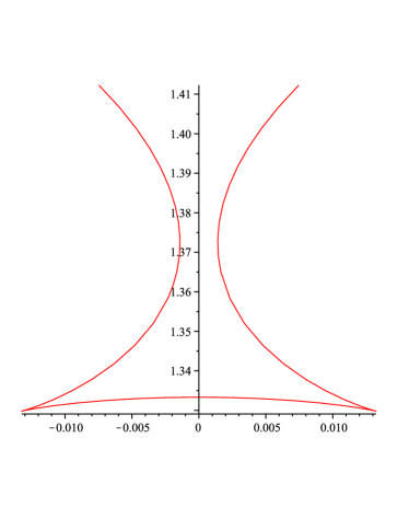
Figure 5: On the left, we show the entire drop for $m=1/3$. On the right, a closeup of upper part of the drop for $m=0.94$. The swallowtail has opened, and there is no more self-intersection.

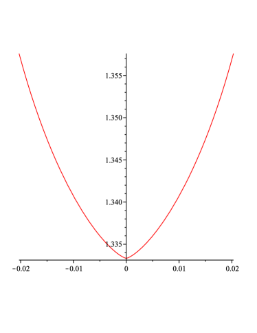
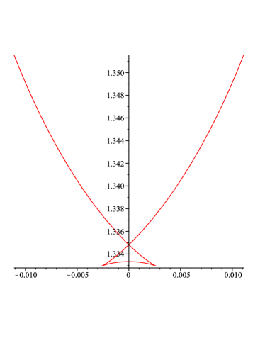
Figure 6: The birth of the swallowtail, as described by (53). For $m=1$ (left) one is exactly at the transition, for $m=0.98$ (right) one finds a swallowtail.

Another exact solution of potential flow that exhibits a cusp, but in the presence of gravity was found by Craya and Sautreaux Craya (1949); Sautreaux (1901); Dun and Hocking (1995); liquid is layered above a two-dimensional ridge. At the crest of the ridge, which has opening angle $2\pi\gamma$, there is a sink. For the special case $\gamma=1/3$ there is an exact solution, given by

$$\frac{dz}{dl}=-i(2/3)^{1/3}\frac{1-l}{l^{1/3}(1+l)^{4/3}},$$ (56)

where $l=\exp(-i\theta)$, $-\pi\leq\theta\leq\pi$. From a local analysis we find that

$$x=-\frac{3^{2/3}}{36}\theta^{3},\quad y=-\frac{3^{2/3}}{12}\theta^{2},$$ (57)

which is once more a 2/3 cusp. Of course this is to be expected, since gravity cannot change the local behavior near a cusp. However it is not clear where this comes from in terms of the swallowtail described above.

V Porous medium equation

Another problem, closely related to the above, concerns the two-dimensional flow of oil in a porous medium. The oil is layered above heavier water, and is withdrawn through a sinkhole. The interface between the oil and the water is deformed, and forms a cusp at a critical flow rate. Inside the oil domain, one has to solve Laplace’s equation for the velocity potential, cf. (42). In the stationary case, one has the usual condition of vanishing normal velocity on the free surface. However, from a pressure balance which includes the hydrostatic pressure, one obtains Zhang and Hocking (1996); Zhang et al. (1997):

$$u^{2}+v^{2}=Kv,$$ (58)

where $u,v$ are the horizontal and vertical components of the velocity, respectively.

Once more hodograph methods can be applied, but the problem can be solved only in the critical case at which there is cusp. Namely, in the subcritical case where there interface is smooth, $u=v=0$ at the stagnation point below the sink. In the presence of a singularity, $u=0,v=K$ at the singularity, and the free surface gets mapped onto a circular arc in the hodograph plane. The resulting interface shape is

$$x=-\frac{2}{c\pi^{2}}\int_{-\beta}^{\sigma}\left(\frac{\sqrt{a+1}}{\sigma_{l}}+{\rm arctanh}\sqrt{a+1}\right)\left(\frac{1}{a-\sigma_{l}}-\frac{1}{a-\sigma_{s}}\right)$$ (59)

$$y=\frac{1}{c\pi}\left(\ln\frac{\sigma_{l}-\sigma}{\sigma-\sigma_{s}}-\ln\frac{\sigma_{l}-1+\beta}{1-\beta-\sigma_{s}}\right),$$ (60)

where $\sigma$ parameterizes the curve and $\sigma_{l}$ and $\sigma_{s}$ are determined from implicit equations involving $c$ and $\beta$.

For $\beta=1$ the curve defined by (59),(60) develops into a cusp. A local expansion yields

$$x=A\int_{-1}^{\sigma}\sqrt{1+a}da=\frac{2A}{3}(\sigma+1)^{3/2},$$ (61)

where $A$ is a constant. The $y$-coordinate is linear in $t+1$, thus (61) describes the usual 2/3 cusp. For $\beta<1$ the interface self-intersects, at the line of symmetry, so this appears to be the generic cusp scenario. Numerical results confirm that the curve is smooth before the cusp forms (subcritical case), and a cusp forms in agreement with the exact solution (59),(60).

VI Viscous flow

Here the flow is governed by the Stokes equation, which in two dimensions can be written in terms of the stream function $\psi$, with $u=\psi_{y}$ and $v=-\psi_{x}$. The stream function obeys the biharmonic equation $\triangle^{2}\psi=0$. In a stationary state, which we are considering, the surface of the fluid is a line with $\psi=const$. On this surface, we also have the surface stress condition

$$\sigma_{ij}n_{j}=\gamma\kappa n_{i},$$ (62)

where $\gamma$ is surface tension and $\kappa$ the curvature of the interface. Once more the flow is driven by singularities, such as a vortex dipole Jeong and Moffatt (1992).

A complex formulation of this problem was developed by Richardson Richardson (1968). The stream function is written as

$$\psi=Im(f(z)+\overline{z}g(z)),$$ (63)

where $f$ and $g$ are analytic functions. The boundary conditions at the free surface can be shown to be

$$Im\left[\left(\overline{\frac{dz}{ds}}\right)f(z)+\overline{z}g(z)\right]=\frac{\gamma}{4\eta},\quad f(z)+\overline{z}g(z)=0,$$ (64)

where $\eta$ is the viscosity of the fluid.

In Jeong and Moffatt (1992), the complex formulation (64) was used to calculate the following model problem: a vortex dipole of strength $\alpha$ is located at a distance $d$ below a free surface of infinite extend. Surface tension is included in the description, but the effect of gravity is neglected. The deformation of the free surface by the viscous flow is determined by the capillary number

$$Ca=\frac{\alpha\eta}{d^{2}\gamma},$$ (65)

which measures the ratio of viscous forces over surface tension forces. The solution of the problem is too involved to be presented here. The exact surface shape, in units of $d$, is given by the function

$$x=a\cos\theta+(a+1)\frac{\cos\theta}{1+\sin\theta},$$ (66)

$$y=a(1+\sin\theta).$$ (67)

The parameter $a$ is determined from the equation

$$4\pi Ca=\frac{-a(3a+2)^{2}K(m)}{1+a+\sqrt{-2a(a+1)}},$$ (68)

where

$$m=\frac{2}{(-2a/(a+1))^{1/4}+((a+1)/(-2a))^{1/4}}$$ (69)

and $K$ is the complete elliptic integral of the first kind:

$$K(m)=\int_{0}^{\pi/2}\frac{d\theta}{\sqrt{1-m^{2}\sin^{2}\theta}}.$$ (70)

In (68) we have only reported the form of the equation for the more relevant case $Ca>0$. Asymptotic analysis of (68)-(70) reveals that for large $Ca$,

$$a=-\frac{1}{3}+\epsilon,\quad\epsilon\approx\frac{32}{9}\exp\left\{-16\pi Ca\right\}.$$ (71)

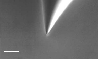
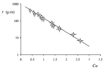
Figure 7: Experimental data on the cusping of a viscous fluid, taken from Lorenceau et al. (2003). On the left, a closeup of the tip of a cusp on the surface of a viscous fluid; the scale bar corresponds to 200 $\mu$ m. On the right, the radius of curvature of the (almost) cusp as function of capillary number. In agreement with (74), the dependence is exponential.

It is easy to confirm that (66) yields a cusp for $a=-1/3$, i.e. for $Ca=\infty$ or vanishing surface tension. If one expands around the cusp point by putting $\theta=\pi/2+\delta$, one obtains

$$x=-\frac{2\epsilon}{3}\delta-\frac{\delta^{3}}{12}$$ (72)

$$y+\frac{2}{3}-2\epsilon=\frac{\delta^{2}}{6},$$ (73)

which is the generic cusp scenario (1). As is apparent from Fig. 1, the case $\epsilon<0$ leads to self-intersection of the free surface, which is of course not physical. The radius of curvature of the cusp for $\epsilon>0$ is given by

$$R\approx\frac{256}{3}\exp\left\{-32\pi Ca\right\},$$ (74)

as found from (72),(71). The exponential dependence (74) has been confirmed experimentally (cf. Fig. 7).

VII Born-Infeld equation

The ideas presented here are not restricted to free surface problems. As an illustration we present a problem that appears in connection with string theory Tseytlin (1999), but is also of long-standing interest in the theory of non-linear waves Whitham (1974). The Born-Infeld equation reads

$$z_{tt}(1+z_{x}^{2})-z_{xx}(1-z_{t}^{2})=2z_{x}z_{t}z_{xt}$$ (75)

Hoppe Hoppe (1995) gave a general solution of the form

$$x^{\prime}(t,\varphi)=\lambda\cos(f-g)\cos(f+g),\quad z^{\prime}(t,\varphi)=\lambda\cos(f-g)\sin(f+g)$$ (76)

$$\dot{x}(t,\varphi)=-\sin(f-g)\sin(f+g),\quad\dot{z}(t,\varphi)=\sin(f-g)\cos(f+g),$$ (77)

where $f=f(\varphi+t/\lambda)$ and $g=g(\varphi-t/\lambda)$ are any two (smooth) functions and $\varphi$ is a parameter. For (76) to be a graph, the tangent vector (76) should not be vertical, i.e. we must require that $|f+g|<\pi/2$.

The curvature of this solution is

$$\kappa(t,\varphi)=\frac{f^{\prime}+g^{\prime}}{\cos(f-g)},$$ (78)

so a singularity is expected whenever $f-g=\pi/2$. Let us assume for simplicity that $g(\zeta)=-f(-\zeta)$. I don’t expect this to be a restriction on the class of possible singularities that can occur. Let $f(\zeta)$ have the local expansion

$$f(\zeta)=\pi/4+a(\zeta-\zeta_{0})-b(\zeta-\zeta_{0})^{2}+O(\zeta-\zeta_{0})^{3},$$ (79)

so together with the symmetry requirement we find

$$f-g=\pi/2+2a(t-\zeta_{0})-2b(\varphi^{2}+(t-\zeta_{0})^{2}).$$ (80)

The factor $\lambda$ can be absorbed into $a$.

From this expression it is clear that $\zeta_{0}$ has to be identified with the singular time $t_{0}$ and $a>0$ for the solution to be regular for $t<t_{0}$. To expand around the singular time, we put $t^{\prime}=t_{0}-t$. Similarly, one must have $b>0$ (otherwise $f-g$ would be $\pi/2$ at an earlier time), and the singularity occurs at $\phi=0$. Thus to leading order we have

$$f-g\approx\pi/2-2at^{\prime}-2b\varphi^{2},\quad f+g\approx 2a\varphi,$$ (81)

from which we get

$$x^{\prime}=2at^{\prime}+2b\varphi^{2},\quad z^{\prime}=4a^{2}t^{\prime}\varphi+4ab\varphi^{3}.$$ (82)

Integrating this expression, using the integrability condition (77), gives

$$x=t^{\prime}\varphi+2c\varphi^{3}/3,\quad z=t^{\prime}\varphi^{2}/2+c\varphi^{4},$$ (83)

where we have used a rescaling of the parameter $\varphi$. This is of course exactly the swallowtail (3) with $\gamma=1$.

References

- Nye (1999) J. Nye, Natural Focusing and Fine Structure of Light: Caustics and Wave Dislocations (Institute of Physics Publishing, Bristol, 1999).
- Arnold (1984) V. I. Arnold, Catastrophe Theory (Springer, 1984).
- Poston and Stewart (1978) T. Poston and I. Stewart, Catastrophe Theory and Its Applications (Dover Publications, Mineola, 1978).
- Berry (1992) M. V. Berry, in Huygens’ principle 1690-1990: Theory and Applications, edited by H. K. K. H. Blok, H. A. Ferwerda (Elsevier, 1992), p. 97.
- Polubarinova-Kochina (1945a) P. Y. Polubarinova-Kochina, Dokl. Akad Nauk USSR 47, 254 (1945a).
- Polubarinova-Kochina (1945b) P. Y. Polubarinova-Kochina, Prikl. Matem. Mech. 9, 79 (1945b).
- Galin (1945) L. A. Galin, Dokl. Akad. Nauk. SSSR 47, 246 (1945).
- Howison (1986) S. D. Howison, SIAM J. Appl. Math 46, 20 (1986).
- Batchelor (1967) G. K. Batchelor, An introduction to Fluid Dynamics (Cambridge University Press, Cambridge, 1967).
- Hopkinson (1898) B. Hopkinson, Proc. Lond. Math. Soc. 29, 142 (1898).
- Kirchhoff (1869) G. Kirchhoff, J. reine angew. Math. 70, 289 (1869).
- Planck (1884) M. Planck, Wied. Ann. 21, 499 (1884).
- Craya (1949) A. Craya, La Houille Blanche 4, 44 (1949).
- Sautreaux (1901) C. Sautreaux, J. Math. Pures Appl. 7, 125 (1901).
- Dun and Hocking (1995) C. R. Dun and G. C. Hocking, J. Engin. Math. 29, 1 (1995).
- Zhang and Hocking (1996) H. Zhang and G. C. Hocking, J. Austral. Math. Soc. B 38, 240 (1996).
- Zhang et al. (1997) H. Zhang, G. C. Hocking, and D. A. Barry, J. Austral. Math. Soc. B 39, 271 (1997).
- Jeong and Moffatt (1992) J.-T. Jeong and H. K. Moffatt, J. Fluid Mech. 241, 1 (1992).
- Richardson (1968) S. Richardson, J. Fluid Mech. 33, 476 (1968).
- Lorenceau et al. (2003) E. Lorenceau, F. Restagno, and D. Quéré, Phys. Rev. Lett. 90, 184501 (2003).
- Tseytlin (1999) A. A. Tseytlin, Born-infeld action, supersymmetry and string theory (1999), URL http://arxiv:hep-th//9908105v5.
- Whitham (1974) G. B. Whitham, Linear and Nonlinear Waves (John Wiley & Sons, 1974).
- Hoppe (1995) J. Hoppe, Conservation laws and formation of singularities in relativistic theories of extended objects (1995), URL http://arxiv:hep-th/9503069.