Water wave collapses over quasi-one-dimensional non-uniformly periodic bed profiles

Abstract

Nonlinear water waves interacting with quasi-one-dimensional, non-uniformly periodic bed profiles are studied numerically in the deep-water regime with the help of approximate equations for envelopes of the forward and backward waves. Spontaneous formation of localized two-dimensional wave structures is observed in the numerical experiments, which looks essentially as a wave collapse.

Nonlinear waves of different nature, when propagating in spatially periodic media, are known to introduce various interesting phenomena. In particular, the so called gap solitons (GSs) can be mentioned, which are self-localized waves existing due to the presence of a Bragg gap in the spectrum of linear waves, and, on the other hand, due to nonlinear interactions between components of the wave field. Gap solitons are studied mainly in the nonlinear optics (see, e.g., Refs.CM1987 ; AW1989 ; CJ1989 ; ESdSKS1996 ; PPLM1997 ; BPZ1998 ; RCT1998 ; CTA2000 ; IdS2000 ; CT2001 ; CMMNSW2008 ), and in the theory of Bose-Einstein condensation EC2003 ; PSK2004 ; MKTK2006 . However, recently it has been suggested that water-wave GSs are possible too, over periodic bottom boundary R2008PRE-2 ; R2008PRE-3 . In the cited works R2008PRE-2 ; R2008PRE-3 , planar potential flows with one-dimensional (1D) free boundary were studied both analytically — with the help of an approximate model possessing relatively simple particular solutions, and numerically — exact equations of motion for an ideal fluid with a free surface over a non-uniform bed were simulated, in terms of the so called conformal variables (see Ref.R2004PRE ). For two horizontal dimensions, the question about possibility of GSs or some other coherent water-wave structures over periodic bed profiles is still open. The present work is a step to study this problem. More specifically, we suggest here approximate equations of motion for a two-dimensional (2D) free surface over a quasi-one-dimensional, locally periodic non-uniform bed. Then we present some numerical results where spontaneous formation of localized nonlinear structures is clearly seen, and the process looks as a kind of wave collapse. It should be emphasized that the Bragg interaction between the forward wave and the backward wave plays the key role in this process, since the wave dynamics over a flat bottom is rather different, and the extreme waves there are not so high as they are with the Bragg interaction. It is quite possible that effects considered in the present work have in some cases relation to the extensively discussed phenomenon of rogue waves Kharif-Pelinovsky ; RogueWaves2006 , namely at seas with a non-uniform depth $\sim 50-100$ m.

Analytical and numerical results of Ref.R2008PRE-3 imply that the most suitable asymptotic regime for observation of nonlinear Bragg structures of the GS type in water-wave systems is the relatively short-wave (or deep-water) regime, when an effective water depth $h_{0}$ and the main Bragg-resonant wave number $\kappa$ form a small parameter $\varepsilon\equiv\exp(-2\kappa h_{0})\sim 0.01$. It should be noted here that the opposite long-wave asymptotic regime is very different, and typical nonlinear structures at shallow water are KdV-type solitons (see, Refs.MeiLi2004 ; GKN2007 ). In the considered deep-water regime, one can use the fourth-order Hamiltonian functional ${\cal H}\{\eta,\psi\}$ for weakly-nonlinear gravity water waves in the approximate form (see Ref.R2008PRE-3 ),

$${\cal H} \approx \frac{1}{2}\int\left\{\psi\hat{K}\psi+g\eta^{2}+\eta\left[(\nabla\psi)^{2}-(\hat{k}\psi)^{2}\right]\right\}d^{2}{\bf r}$$ (1)

$$+ \frac{1}{2}\int\left[\psi\hat{k}\eta\hat{k}\eta\hat{k}\psi+\eta^{2}(\hat{k}\psi)\nabla^{2}\psi\right]d^{2}{\bf r},$$

where ${\bf r}=(x,y)$ is the position in the horizontal plane, $g$ is the gravity acceleration, the canonical variables $\eta({\bf r},t)$ and $\psi({\bf r},t)$ are the vertical coordinate of the free surface and the boundary value of the velocity potential respectively, the linear operator $\hat{k}=(\hat{k}_{x}^{2}+\hat{k}_{y}^{2})^{1/2}$ is diagonal in the Fourier representation, and $\hat{K}=\hat{k}+\hat{B}$ is a linear operator connecting the velocity potential $\varphi(x,y,z=0)$ at the unperturbed free surface and the quantity $\partial_{z}\varphi(x,y,z=0)$, in the presence of an inhomogeneous bed. The operator $\hat{B}$ depends on a given bed profile in a complicated manner (see Refs.RA_Smith1998 ; R2008PRE-3 , where some expansions of this operator are discussed), but it is definitely “small” in the deep-water limit, $\hat{B}\sim\varepsilon$, and that is why we keep $\hat{B}$ only in the quadratic part of the Hamiltonian, while in all higher-order terms we write $\hat{k}$ instead of $\hat{K}$.

Canonical equations of motion, corresponding to Hamiltonian (1), are still too complicated to be treated analytically, and very time-demanding when being solved numerically. Therefore we shall consider here a simplified model which can be derived from (1) in some limit. To do this, let us recall the well known fact that a suitable weakly nonlinear canonical transformation,

$$b_{\bf k}=\frac{\sqrt{g}\eta_{\bf k}+i\sqrt{|{\bf k}|}\psi_{\bf k}}{\sqrt{2\omega_{\bf k}}}+\mbox{ nonlinear terms},$$ (2)

(where $\omega_{\bf k}=(g|{\bf k}|)^{1/2}$ is a linear dispersion relation in the absence of the bottom boundary) can exclude the third-order terms from the deep-water Hamiltonian, as well as the non-resonant wave interactions $0\leftrightarrow 4$ and $1\leftrightarrow 3$ (see Refs.K1994 ; Z1999 ). Accordingly, the shape of the free surface $\eta(x,y,t)$ is given by the formula below:

$$\eta({\bf r},t)=\mbox{Re}\int\left(\frac{2\omega_{\bf k}}{g}\right)^{1/2}b_{\bf k}(t)e^{i{\bf kr}}d{\bf k}/(2\pi)+\cdots.$$ (3)

In terms of the new normal complex variables $b_{\bf k}(t)$, the wave dynamics in deep-water regime is described by the following integral equation,

$$i\dot{b}_{\bf k} \approx \omega_{\bf k}b_{\bf k}+\hat{L}b_{\bf k}+\dots+\frac{1}{2}\int T({\bf k},{\bf k}_{2};{\bf k}_{3},{\bf k}_{4})b^{*}_{{\bf k}_{2}}b_{{\bf k}_{3}}b_{{\bf k}_{4}}$$ (4)

$$\qquad\qquad\times\delta({\bf k}+{\bf k}_{2}-{\bf k}_{3}-{\bf k}_{4})\,d{\bf k}_{2}\,d{\bf k}_{3}\,d{\bf k}_{4},$$

where $\hat{L}$ is a “small” linear non-diagonal operator related to $\hat{B}$, and $T({\bf k}_{1},{\bf k}_{2};{\bf k}_{3},{\bf k}_{4})$ is a known continuous function (but the corresponding explicit expression is rather complicated, see Refs.K1994 ; Z1999 ). For our purposes it is sufficient to know that in purely one-dimensional case

$$T(k_{1},k_{2};k_{1},k_{2})\propto|k_{1}||k_{2}|(|k_{1}+k_{2}|-|k_{1}-k_{2}|),$$ (5)

and thus $T(k,-k;k,-k)=-T(k,k;k,k)<0$.

Let us assume for the moment that a bed profile is strictly $x$-periodic, with the period $\Lambda=\pi/\kappa$, and a 1D wave spectrum is concentrated near the Bragg-resonant wave vectors $\pm{\bf k}_{0}=\pm\kappa{\bf e}_{x}$. Now we introduce two slowly-$x$-dependent functions, the envelopes $A_{\pm}(x,t)$ of the forward- and backward-propagating waves,

$$\eta(x,t)=\mbox{Re}[A_{+}\exp(i\kappa x-i\tilde{\omega}t)+A_{-}\exp(-i\kappa x-i\tilde{\omega}t)],$$

where $\tilde{\omega}=(g\kappa)^{1/2}$ (the corresponding deep-water wave period is $T_{0}=2\pi/\tilde{\omega}$). Then we take into account only the main-order components of the integral operator $\hat{L}$:

$$L_{{\bf k}_{0},{\bf k}_{0}}=L_{-{\bf k}_{0},-{\bf k}_{0}}=-\tilde{\omega}\varepsilon,\quad L_{{\bf k}_{0},-{\bf k}_{0}}=L^{*}_{-{\bf k}_{0},{\bf k}_{0}}=\tilde{\omega}\Delta,$$

where $\varepsilon$ is a real positive number, which should be identified as $\varepsilon=\exp(-2\kappa h_{0})$, for some efficient depth $h_{0}$, since the finite-depth dispersion relation is $\omega=[g\kappa\tanh(h_{0}\kappa)]^{1/2}\approx\tilde{\omega}[1-\exp(-2\kappa h_{0})]$; a complex parameter $\Delta=|\Delta|\exp(i\phi_{0})$ bears information about the width of the main Bragg gap (namely, the edges of the frequency gap are at $\omega_{1,2}\approx\tilde{\omega}(1-\varepsilon\mp|\Delta|$), and about the phase $\phi_{0}$ of the main Fourier harmonics of the bed undulation in some suitable representation (see Ref.R2008PRE-3 for details). It is worth mentioning that for all 1D bed profiles considered in the previous studies R2008PRE-2 ; R2008PRE-3 , the inequality $|\Delta|<\varepsilon$ holds ($|\Delta|$ approaches $\varepsilon$ from the below if the bottom boundary consists of very narrow barriers).

As a result of the standard procedure, we obtain the system of two coupled approximate equations for the wave envelopes $A_{\pm}(x,t)$ (compare to Ref.R2008PRE-3 ),

$$i\Big{(}\frac{\partial_{t}}{\tilde{\omega}}+\frac{\partial_{x}}{2\kappa}+\cdots\Big{)}A_{+}=\Delta\,A_{-}-\varepsilon A_{+}$$

$$\qquad\qquad+\frac{\kappa^{2}}{2}\left(|A_{+}|^{2}-2|A_{-}|^{2}\right)A_{+},$$ (6)

$$i\Big{(}\frac{\partial_{t}}{\tilde{\omega}}-\frac{\partial_{x}}{2\kappa}+\cdots\Big{)}A_{-}=\Delta^{*}\,A_{+}-\varepsilon A_{-}$$

$$\qquad\qquad+\frac{\kappa^{2}}{2}\left(|A_{-}|^{2}-2|A_{+}|^{2}\right)A_{-},$$ (7)

where the dots mean the second- and higher-order $x$-derivatives. The above equations describe weakly nonlinear 1D water-wave GSs quite well: known solitary-wave solutions of this system were compared in Ref.R2008PRE-3 to numerical simulations of the exact equations of motion for an ideal fluid with a free surface, and a reasonable correspondence was found.

Now it is clear how to generalize the above system to the 2D case: we have just to add $\partial_{y}$-dependent dispersive terms to the left hand sides, which appear from expansions of the operators $[-\kappa^{-1/2}((-i\partial_{x}\pm\kappa)^{2}-\partial_{y}^{2})^{1/4}+1]$. Moreover, we shall consider here the case when $\varepsilon$ and $\Delta$ are no longer constants, but they are some functions slowly depending on the horizontal coordinates $x$ and $y$. This assumption makes our model more realistic and rich, since there is no perfectly periodic bed structures in the nature, while roughly periodic bars are quite often. Then the following natural generalization of Eqs.(Water wave collapses over quasi-one-dimensional non-uniformly periodic bed profiles-Water wave collapses over quasi-one-dimensional non-uniformly periodic bed profiles) can be suggested,

$$\Big{(}\frac{i\partial_{t}}{\tilde{\omega}}+\frac{i\partial_{x}}{2\kappa}-\frac{\partial_{x}^{2}}{8\kappa^{2}}+\frac{\partial_{y}^{2}}{4\kappa^{2}}+\cdots\Big{)}A_{+}=-\varepsilon(x,y)A_{+}$$

$$\qquad+\Delta(x,y)A_{-}+\frac{\kappa^{2}}{2}\left(|A_{+}|^{2}-2|A_{-}|^{2}\right)A_{+},$$ (8)

$$\Big{(}\frac{i\partial_{t}}{\tilde{\omega}}-\frac{i\partial_{x}}{2\kappa}-\frac{\partial_{x}^{2}}{8\kappa^{2}}+\frac{\partial_{y}^{2}}{4\kappa^{2}}+\cdots\Big{)}A_{-}=-\varepsilon(x,y)A_{-}$$

$$\qquad+\Delta^{*}(x,y)A_{+}+\frac{\kappa^{2}}{2}\left(|A_{-}|^{2}-2|A_{+}|^{2}\right)A_{-},$$ (9)

where the dots mean omitted third- and higher-order partial derivatives. We keep here the second-order dispersive terms because they are definitely important in the dynamics of relatively short wave groups. The linear and nonlinear terms in the right hand sides are of the same order of magnitude at $\kappa|A_{\pm}|\sim 0.1$ and $\varepsilon\sim|\Delta|\sim 0.01$ (let us note that water waves become strongly nonlinear if $\kappa|A_{\pm}|\gtrapprox 0.3$). The above equations have the standard Hamiltonian structure, $i\tilde{\omega}^{-1}\partial_{t}A_{\pm}=\delta\tilde{\cal H}/\delta A^{*}_{\pm}$, with

$$\tilde{\cal H} = \int[A^{*}_{+}\hat{D}_{+}A_{+}+A^{*}_{-}\hat{D}_{-}A_{-}]d^{2}{\bf r}$$ (10)

$$+ \int[\Delta A^{*}_{+}A_{-}+\Delta^{*}A^{*}_{-}A_{+}-\varepsilon(A^{*}_{+}A_{+}+A^{*}_{-}A_{-})]d^{2}{\bf r}$$

$$+ \kappa^{2}\int[(|A_{+}|^{4}+|A_{-}|^{4})/4-|A_{+}|^{2}|A_{-}|^{2}]d^{2}{\bf r},$$

where the dispersive operators $\hat{D}_{\pm}$ are

$$\hat{D}_{\pm}=\mp{i\partial_{x}}/({2\kappa})+{\partial_{x}^{2}}/({8\kappa^{2}})-{\partial_{y}^{2}}/({4\kappa^{2}})+\cdots$$ (11)

It should be emphasized that a (spatially non-uniform) linear Bragg coupling between the forward wave and the backward wave introduces essentially new effects in the dynamics, in comparison with the flat-bottom case. It is already seen from the linear-wave dispersion relations corresponding to the simplest case $\varepsilon=const$ and $\Delta=const>0$. There are two branches in the spectrum (type-1 and type-2 waves), behaving quite non-trivially,

$$\tilde{\omega}^{-1}\Omega_{1,2}({\bf k})=-\varepsilon\pm\sqrt{\Delta^{2}+\frac{k_{x}^{2}}{4\kappa^{2}}}+\frac{k_{y}^{2}}{4\kappa^{2}}-\frac{k_{x}^{2}}{8\kappa^{2}}+\dots$$ (12)

Various nonlinear processes occur in this system, which create instabilities near corresponding resonant curves in ${\bf k}$-plane. For example, two type-1 waves with ${\bf k}_{1}={\bf 0}$ decay into two type-2 waves with wave vectors $\pm{\bf k}_{2}$ ($2\leftrightarrow 2$ process), if

$$2\Omega_{1}({\bf 0})\approx\Omega_{2}({\bf k}_{2})+\Omega_{2}(-{\bf k}_{2}).$$ (13)

Thus, a spatially homogeneous solution $A_{+}=A_{-}=A_{0}\exp(-i\Omega_{0}t)$, with a small but finite constant amplitude $A_{0}$, is unstable. A standard linear analysis shows that a maximum of the instability increment is reached at the perpendicular direction, near ${\bf k}_{2}=\pm{\bf e}_{y}\kappa\sqrt{8\Delta}$. Moreover, besides the above indicated instability, there is another, long-scale modulation instability of type-1 waves, which completely surrounds the wave vector ${\bf k}=0$, unlike the situation for oppositely propagating waves at infinitely deep water (see, e.g., Refs.ORS2006 ; SKEMS2006 ). Therefore the tendency towards spontaneous formation of big waves is more strong if the bottom is (locally) periodic. However, a more detailed analytical study of Eqs.(8-9), including full stability analysis and particular solutions, will be a subject of future research. In this work we only present results of numerical simulations which give a general impression about the dynamics, with particular attention to the phenomenon of wave collapses.

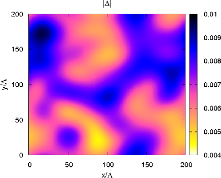
Figure 1: (Color online). The absolute value of $\Delta(x,y)$.

Figure 2: The global maximum of wave amplitude versus time.

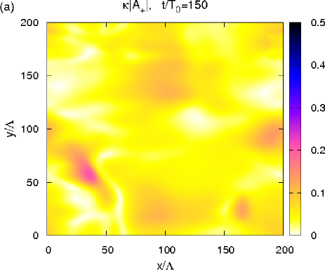
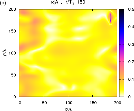
Figure 3: (Color online). The absolute values $|A_{\pm}(x,y,t)|$ at $t/T_{0}=150$. The localized energetic structure is seen near the right upper corner of the $|A_{-}|$ map.

The numerical simulations were performed in the standard dimensionless square domain $2\pi\times 2\pi$, with periodic boundary conditions and with $\kappa=100$. In this example, function $\varepsilon$ was taken in the form $\varepsilon=0.014(1+0.1\cos x+0.1\cos y)$, while $\Delta(x,y)=0.007[1+0.05\xi(x,y)]$ was used, where a complex function $\xi(x,y)$ contained discrete Fourier harmonics within $-5\leq k_{x}\leq 5$ and $-5\leq k_{y}\leq 5$, with amplitudes decaying as $\exp[-0.1(k_{x}^{2}+k_{y}^{2})]$ and with pseudo-random phases (see Fig.1, where a map of the absolute value $|\Delta(x,y)|$ is shown). The initial conditions were $\kappa A_{+}=0.08+a_{+}(x,y)$ and $\kappa A_{-}=a_{-}(x,y)$, where functions $a_{\pm}(x,y)$ had the Fourier spectra with amplitudes behaving as $0.001\exp[-0.04(k_{x}^{2}+k_{y}^{2})]$ and with pseudo-random phases. Thus, the most part of wave energy was initially concentrated in the forward wave. However, after few tens of wave periods, the energy has been redistributed between the forward and backward waves due to the inhomogeneous Bragg coupling. Wide regions of slightly higher wave amplitude were formed, as a result of interplay between random initial conditions and random $\Delta$, which process is reflected in Fig.2. After that, self-focusing nonlinear interactions came into play and rapidly produced the big wave which is seen in Fig.3. It is interesting to note that the localized structure was developed only in one of the two wave envelopes: there is no clear sign of the same big wave in the opposite-wave amplitude.

The $x$-size of the developed high wave group contains just 1-2 wave lengths, while the $y$-size is larger, about 10 wave lengths. Strictly speaking, the assumption of narrow spectra for $A_{\pm}$ is violated in this situation, so the system (8-9) can describe the final stage of wave collapse only qualitatively. To get indirect confirmations for the wave collapses, we compared the above approximate results to analogous simulations of full systems of the type (4), for some simple functions $T_{m}({\bf k}_{1},{\bf k}_{2};{\bf k}_{3},{\bf k}_{4})$ which possess the same property (5) and thus mimic the true complicated matrix element $T({\bf k}_{1},{\bf k}_{2};{\bf k}_{3},{\bf k}_{4})$. In particular, we considered

$$T_{m}\propto|{\bf k}_{1}|^{\frac{1}{2}}|{\bf k}_{2}|^{\frac{1}{2}}|{\bf k}_{3}|^{\frac{1}{2}}|{\bf k}_{4}|^{\frac{1}{2}}(|{\bf k}_{1}+{\bf k}_{2}|+|{\bf k}_{3}+{\bf k}_{4}|$$

$$-|{\bf k}_{1}-{\bf k}_{3}|-|{\bf k}_{1}-{\bf k}_{4}|-|{\bf k}_{2}-{\bf k}_{3}|-|{\bf k}_{2}-{\bf k}_{4}|),$$ (14)

and there the wave collapses were observed as well (we do not discuss here subtle points related to such systems). In the reality, however, higher-order nonlinearities become important at $|\kappa A_{\pm}|\gtrapprox 0.3$ and they produce wave breaking manifested as the well-known “white caps”. Therefore the question about maximal wave height at the finite stage of collapse can be fully answered only through real-world experiments.

To conclude, in the present work we have derived and then numerically simulated nonlinear equations of motion for complex water-wave amplitudes coupled both linearly through the (spatially non-uniform) Bragg interaction, and non-linearly through the cross-modulation terms. In the numerical experiments, we have observed spontaneous formation of highly energetic localized structures which look like wave collapses rather than like solitons. The final stage of these wave collapses is actually beyond applicability of our weakly-nonlinear model. That is why some real-world experiments or at least fully nonlinear simulations are desirable. Unfortunately, large-scale simulations in the framework of the exact Eulerian dynamics, for instance with the help of the existing boundary integral methods, are hardly possible at the moment because of their extremely time-demanding implementations. Perhaps, the weakly non-planar but fully nonlinear equations of motion for potential water waves over quasi-one-dimensional topography, derived in Ref.R2005PRE , might be useful as an intermediate step towards accurate numerical results.

These investigations were supported by RFBR (grants 09-01-00631 and 07-01-92165), by the “Leading Scientific Schools of Russia” grant 4887.2008.2, and by the Program “Fundamental Problems of Nonlinear Dynamics” from the RAS Presidium.

References

- (1) W. Chen and D.L. Mills, Phys. Rev. Lett. 58, 160 (1987).
- (2) A. B. Aceves and S. Wabnitz, Phys. Lett. A 141, 37 (1989).
- (3) B. J. Eggleton, R. E. Slusher, C. M. de Sterke et al., Phys. Rev. Lett. 76, 1627 (1996).
- (4) D.N. Christodoulides and R.I. Joseph, Phys. Rev. Lett. 62, 1746 (1989).
- (5) T. Peschel, U. Peschel, F. Lederer, and B. A. Malomed, Phys. Rev. E 55, 4730 (1997).
- (6) I.V. Barashenkov, D.E. Pelinovsky, and E.V. Zemlyanaya, Phys. Rev. Lett. 80, 5117 (1998).
- (7) A. de Rossi, C. Conti, and S. Trillo, Phys. Rev. Lett. 81, 85 (1998).
- (8) C. Conti, S. Trillo, and G. Assanto, Phys. Rev. Lett. 85, 2502 (2000).
- (9) T. Iizuka and C. Martijn de Sterke, Phys. Rev. E 61, 4491 (2000).
- (10) C. Conti and S. Trillo, Phys. Rev. E 64, 036617 (2001).
- (11) K. W. Chow, I. M. Merhasin, B. A. Malomed et al., Phys. Rev. E 77, 026602 (2008).
- (12) N. Efremidis and D. N. Christodoulides, Phys. Rev. A 67, 063608 (2003).
- (13) D. E. Pelinovsky, A. A. Sukhorukov, and Yu. S. Kivshar, Phys. Rev. E 70, 036618 (2004).
- (14) M. Matuszewski, W. Krolikowski, M. Trippenbach, and Y. S. Kivshar, Phys. Rev. A 73, 063621 (2006).
- (15) V. P. Ruban, Phys. Rev. E 77, 055307(R) (2008).
- (16) V. P. Ruban, Phys. Rev. E 78, 066308 (2008).
- (17) V. P. Ruban, Phys. Rev. E 70, 066302 (2004).
- (18) C. Kharif and E. Pelinovsky, Eur. J. Mech. B/Fluids 22, 603 (2003).
- (19) Special Issue: Eur. J. Mech. B/Fluids 25, 535-692 (2006).
- (20) C. C. Mei and Y. Li, Phys. Rev. E 70, 016302 (2004).
- (21) J. Garnier, R. A. Kraenkel, and A. Nachbin, Phys. Rev. E 76, 046311 (2007).
- (22) R. A. Smith, J. Fluid Mech. 363, 333 (1998).
- (23) V. P. Krasitskii, J. Fluid Mech. 272, 1 (1994).
- (24) V. Zakharov, Eur. J. Mech. B/Fluids 18, 327 (1999).
- (25) M. Onorato, A. R. Osborne, and M. Serio, Phys. Rev. Lett. 96, 014503 (2006).
- (26) P. K. Shukla, I. Kourakis, B. Eliasson et al., Phys. Rev. Lett. 97, 094501 (2006).
- (27) V. P. Ruban, Phys. Rev. E 71, 055303(R) (2005).