Towards a fully consistent Milky Way disc model: Part 1 The local model based on kinematic and photometric data.

Abstract

We present a fully consistent evolutionary disc model of the solar cylinder. The model is based on a sequence of stellar sub-populations described by the star formation history (SFR) and the dynamical heating law (given by the age-velocity dispersion relation AVR). The stellar sub-populations are in dynamical equilibrium and the gravitational potential is calculated self-consistently including the influence of the dark matter halo and the gas component. The combination of kinematic data from Hipparcos and the finite lifetimes of main sequence (MS) stars enables us to determine the detailed vertical disc structure independent of individual stellar ages and only weakly dependent on the IMF. The disc parameters are determined by applying a sophisticated best fit algorithm to the MS star velocity distribution functions in magnitude bins. We find that the AVR is well constrained by the local kinematics, whereas for the SFR the allowed range is larger. The model is consistent with the local kinematics of main sequence stars and fulfils the known constraints on scale heights, surface densities and mass ratios. A simple chemical enrichment model is included in order to fit the local metallicity distribution of G dwarfs. In our favoured model A the power law index of the AVR is 0.375 with a minimum and maximum velocity dispersion of 5.1 km/s and 25.0 km/s, respectively. The SFR shows a maximum 10  Gyr ago and declines by a factor of four to the present day value of 1.5 $\rm{M}_{\mathrm{\rm\sun}}/\mathrm{pc}^{2}/\mathrm{Gyr}$. A best fit of the IMF leads to power-law indices of -1.46 below and -4.16 above 1.72$\rm{M}_{\mathrm{\rm\sun}}$ avoiding a kink at 1$\rm{M}_{\mathrm{\rm\sun}}$. An isothermal thick disc component with local density of $\sim 6\%$ of the stellar density is included. A thick disc containing more than 10% of local stellar mass is inconsistent with the local kinematics of K and M dwarfs. Neglecting the thick disc component results in slight variations of the thin disc properties, but has a negligible influence on the AVR and the normalised SFR. The model allows detailed predictions of the density, age, metallicity and velocity distribution functions of MS stars as a function of height above the mid-plane. The complexity of the model does not allow to rule out other star formation scenarios using the local data alone. The incorporation of multi-band star count and kinematic data of larger samples in the near future will improve the determination of the disc structure and evolution significantly.

1 Introduction

There is no ’concordance’ Milky Way model available so far that describes the structure, kinematics, chemistry and evolution of the disc in great detail. The classical stellar density model of Bahcall & Soneira (1980a, b, 1984) composed by a spheroid and an exponential disc with magnitude-dependent exponential scale heights is still widely used. Bahcall (1984a, b) introduced a finite set of isothermal disc components and solved the Poisson and the Jeans equation for a dynamical equilibrium model of the vertical disc structure. At present the most sophisticated Milky Way model based on star counts is the so-called ’Besançon model’ of the Galaxy developed and presented in a series of articles. In Robin et al. (2003) a general description and the present status of the model is given. In this model the thin disc is composed by a sequence of stellar sub-populations with increasing age and velocity dispersion. The Besançon model has still some serious drawbacks in the construction of the thin disc concerning the density profiles of the components, the star formation history (SFR) and the initial mass function (IMF) that will be discussed below.

The main input functions to be determined in an evolutionary disc model are the SFR and the dynamical heating described by the age-velocity dispersion relation (AVR). The $\mathrm{SFR}(t)$ of the Milky Way disc is still not very well determined. The main reason for that is the lack of good age estimators with corresponding unbiased stellar samples. Especially samples selected by colour cuts or by a magnitude limit are biased with respect to the age distribution, because there is an age-metallicity relation due to the chemical enrichment of the disc. Therefore not even the famous Geneva-Copenhagen sample of 14,000 F and G stars (Nordström et al., 2004; Holmberg et al., 2009) (hereafter GCS1,GCS2) with well determined stellar properties and individual age estimates can be used to derive the star formation history directly by star counts. Systematic biases introduced by the method of GCS1 concerning age and stellar parameter determinations are discussed in Pont & Eyer (2005) and Haywood (2006). The Besançon model of the Galaxy was developed and presented in a series of articles. In Haywood et al. (1997a, b) the SFR of the thin disc is determined to be approximately constant using a series of isothermal components and applying an approximate method to achieve dynamical equilibrium. In further applications they used a constant SFR combined with a steep IMF in the sensitive mass regime of 1-3 $\rm{M}_{\mathrm{\rm\sun}}$ (Robin et al., 2003). As a result, the mean age of the disc population, the scale heights and the surface densities of the stellar sub-populations are relatively small. Rocca-Pinto et al. (2000) used chromospheric age determinations of late-type dwarfs. They apply stellar evolution and scale height corrections. The main result is the determination of enhanced star formation episodes over the lifetime of the disc. They exclude a constant SFR from chemical evolution models. In R. & C. de la Fuente Marcos (2004) the star formation history for open star clusters was determined. They found at least five episodes of enhanced star formation in the last 2 Gyr. Since star clusters contain only a small percentage of all disc stars, an extrapolation to the total (smoothed) SFR is not possible.

In recent years the Hipparcos stars with precise parallaxes and proper motions were used to determine the SFR with different methods. Hernandez et al. (2000) determined the SFR over the last 3 Gyr using isochrone ages. They found a series of star formation episodes on top of an underlying smooth SFR. This result is complementary to our model, which gives the slow evolution of the smoothed SFR. Vergely et al. (2002) applied an inverse method to derive from the colour magnitude diagram the star formation history and age-metallicity relation. They used prescribed AVR and gravitational potential and fixed the IMF to be a power law over the whole stellar mass range. This ansatz results in a steep IMF and a rather young thin disc. Additionally they found strong maxima in the SFR at ages of $10^{7}$ and $2\times 10^{9}$ yr. In Binney et al. (2000) and in Cignoni et al. (2006) the scale height variation of main sequence stars was not taken into account. Therefore these models derive the local age distribution of stellar sub-populations with lifetimes larger than the age of the disc instead of the SFR. Binney et al. (2000) determined the age of the solar neighbourhood to be $11.2\pm 0.75$ Gyr, which includes the contribution of the thick disc. Both papers found an approximately constant local age distribution, which corresponds to a decreasing SFR according to the increasing scale height with increasing age of the stellar sub-populations. In a recent paper Aumer & Binney (2009) derived the SFR using the updated Hipparcos data (van Leeuwen, 2007) and the kinematics of the GCS sample. They calculated in detail the number of main sequence (MS) stars as function of B-V colour based on a KTG93-like IMF and scale height corrections due to dynamical heating. Their favoured disc model has an exponentially decaying SFR with a decay timescale of 8.5 Gyr and an age of 12.5 Gyr. In the model the gravitational potential is fixed and the SFR depends strongly on the properties of the IMF by construction.

The presented paper (Paper I) starts a new attempt to develop a fully consistent disc model which is able to predict the properties of the Milky Way disc in great detail concerning density distributions, age distributions, kinematics and chemistry of all types of stars. The aim of this sequence of papers is to construct a smooth physically consistent disc model that can be extended to a global Galaxy model and allows detailed predictions of number densities and kinematics of stars of different types. The new model can be of some help for the construction of a ’concordance’ model of the Milky Way. It can be used for the preparation of the future astrometric space mission Gaia that will measure with high precision positions, distances, proper motions and stellar parameters (temperature, surface gravity and chemical composition) of one billion stars (Perryman et al., 2001; Bailer-Jones, 2005).

We start with a local disc model of the solar cylinder, which is based on the SFR, the AVR and a chemical evolution function described by the age-metallicity-relation (AMR). The vertical density profiles and the corresponding scale height determinations of thin and thick disc stars are calculated in a self-consistent gravitational potential including the DM halo and the gas component. The model parameters are determined by a best fit procedure of the velocity distribution functions $f_{\mathrm{i}}(|W|)$ of solar neighbourhood stars from B–K dwarfs. We use Hipparcos stars and at the faint end the Catalogue of Nearby Stars (CNS4), select the MS stars and divide these into a series of volume complete sub-samples in magnitude bins. The derived $f_{\mathrm{i}}(|W|)$ of each sub-sample are compared simultaneously to the model predictions. Details of the fitting procedure and the significance with respect to parameter variations are discussed in a future paper (Just & Jahreiß, 2009) (Paper II).

Since the velocity distribution function of MS samples is the average over the lifetime of these stars properly weighted by the SFR and the dilution due to the increasing scale height, the time resolution is strongly limited. Therefore we use only smooth input functions for the SFR, AVR and metal enrichment in the model. The resulting SFR, AVR and chemical evolution describe the long-term smoothed disc evolution. Similar disc models by fitting the vertical luminosity and colour profiles of edge-on galaxies instead of the kinematics have already been used successfully (Just et al., 1996, 2006).

The main advantages of this method is that it does not depend on individual stellar age determinations and that it is essentially independent of the shape of the IMF. A weakness is that we cannot confine the SFR strongly based on local data only. The application of the model to star counts of remote stellar populations will be of great help in this respect. In subsequent work the local model will be continuously extended and compared to large data samples taken from the Sloan Digital Sky Survey SDSS/SEGUE (Abazajian et al., 2009) and the Radial Velocity Experiment RAVE (Zwitter et al., 2008) to further constrain the possible parameter range of the disc model.

A major restriction of a local model is that radial mixing of stars in the disc cannot be included easily. There are two main mixing processes discussed in the literature. The first one is directly connected to the dynamical heating process responsible for the AVR. The gravitational scattering process leads to a diffusion of orbits in velocity space (AVR) and in position (radial, tangential, vertical mixing). Wielen et al. (1996) discussed the radial diffusion of stellar orbits and the consequences for the AMR in some detail. The radial probability distribution function of the birth-places depends mainly on the age of the stellar sub-population and only weakly on the physical scattering process. For a 5 Gyr old population the typical radial width of the initial distribution is $\pm 2$ kpc. The second mechanism is resonant scattering of circular orbits by spiral arms (Sellwood & Binney, 2002; Roskar et al., 2008; Schönrich & Binney, 2009). This mechanism changes the radial position of stars quickly, but the eccentricity of the orbits remain very small. The effect of resonant scattering may account for up to half the stars in the solar neighborhood (Roskar et al., 2008), which shows the possible scale of the errors which may result if migration is ignored. Unfortunately the efficiency and the properties of resonant scattering in the Milky Way disc are still poorly known. In a future global disc model radial mixing may be included in a parametrized form. The local model presented in this paper is primarily a description of the ’status quo’ of the local Milky Way disc quantified by the local age distribution (SFR), the kinematics (AVR) and the chemical composition (AMR). Therefore the relations between these function are not altered by radial mixing. But the physical interpretation of the SFR as a ’local star formation history’ and the AVR as a ’local dynamical heating process’ are weakened by radial mixing and require corrections. For the chemical evolution model the consequences are more severe. The tight connection of the enrichment, the SFR and the gas infall will be broken. The chemical enrichment of the gas decouples partly from the (apparent) enrichment of the stellar population. A more general local AMR including an intrinsic scatter would be the consequence as derived by Schönrich & Binney (2009).

In section 2 the physics of the disc model is presented, section 3 describes the observational data, in section 4 the fitting procedure and the properties of the best fit models are given, section 5 collects the main results and discussion.

2 Disc Model

In this section we describe the construction of the disc model and the determination of the properties of the stellar sub-samples. We use a thin, self-gravitating disc composed of a sequence of stellar sub-populations according to the SFR and the AVR as input functions. Additionally the gravitational force of the gas component and the DM halo are included. The bulge and the stellar halo can be neglected in the solar neighbourhood. The total gravitational potential and the density profile of each age-bin are determined self-consistently assuming isothermal distribution functions with velocity dispersion according to the AVR. We take into account finite stellar lifetimes and mass loss due to stellar evolution. The stellar remnants stay in their sub-population, the expelled gas (stellar winds, PNs, and SNs) is mixed implicitly into the gas component. Since the lifetimes and mass loss depend on metallicity, the metal enrichment with time is included. A standard IMF is used for the determination of the stellar mass fraction of the sub-populations with age. The velocity distribution functions $f_{\mathrm{ms}}(|W|)$ for main sequence stars are calculated by a superposition of the Gaussians weighted by the local density contribution up to the lifetime of the stars.

2.1 Self-gravitating disc

The backbone of the disc is a self-gravitating vertical disc profile in the thin disc approximation including the gas component and the DM halo. In this approximation the Poisson-Equation is one-dimensional and in the case of a purely self-gravitating thin disc (i.e. no external potential) the Poisson equation can be integrated leading to

$$\left(\frac{\mbox{\rm d}\Phi}{\mbox{\rm d}z}\right)^{2}=8\pi G\int_{0}^{\Phi}\rho(\Phi^{\prime})\mbox{\rm d}\Phi^{\prime}\quad.$$ (1)

Therefore we model all gravitational components by a thin disc approximation. We include in the total potential $\Phi$ the contributions of the stellar component $\Phi_{\mathrm{s}}$, the gas component $\Phi_{\mathrm{g}}$, and the DM halo $\Phi_{\mathrm{h}}$

$$\Phi(z)=\Phi_{\mathrm{s}}(z)+\Phi_{\mathrm{g}}(z)+\Phi_{\mathrm{h}}(z)\quad.$$ (2)

In order to obtain the force of a spherical halo correctly in the thin disc approximation, we use a special approximation (see subsection 2.4). Since we construct the disc in dynamical equilibrium, the density of the sub-components are given as a function of the total potential $\rho_{\mathrm{j}}(\Phi)$. The vertical distribution is given by the implicit function $z(\Phi)$ via direct integration

$$z(\Phi)=\int_{0}^{\Phi}\mbox{\rm d}\Phi^{\prime}\left[8\pi G\int_{0}^{\Phi^{\prime}}\rho(\Phi^{\prime\prime})\mbox{\rm d}\Phi^{\prime\prime}\right]^{-1/2}\quad.$$ (3)

For the fitting procedure it is essential to separate the normalised model and the scaling factors. Since we use the SFR and the AVR as input functions, it is convenient to normalise the model to the total surface density $\Sigma_{\mathrm{tot}}$ and to the maximum velocity dispersion $\sigma_{\mathrm{e}}$ of the oldest thin disc sub-population. As a consequence the gravitational potential in equations 1 and 3 is normalised to $\sigma_{\mathrm{e}}^{2}$ and a natural scale length is

$$z_{\mathrm{e}}=\frac{\sigma_{\mathrm{e}}^{2}}{2\pi G\Sigma_{\mathrm{tot}}},$$ (4)

which corresponds to the exponential scale height of an isothermal component with velocity dispersion $\sigma_{\mathrm{e}}$ above a gravitating sheet with total surface density $\Sigma_{\mathrm{tot}}$.

The normalised disc model describes the intrinsic structure of the disc. The relative thin disc, thick disc, gaseous, and DM fractions of the surface density (up to $|z|=z_{\mathrm{max}}$) are given by the input parameters $Q_{\mathrm{s}},Q_{\mathrm{t}},Q_{\mathrm{g}},Q_{\mathrm{h}}$ that have to be iterated to find the best model. The value of $z_{\mathrm{max}}$ is determined by the prescribed maximum of the normalised potential $\Phi(z_{\mathrm{max}})/\sigma_{\mathrm{e}}^{2}$. The disc model has two free global scaling parameters to convert the normalised model to physical quantities. One can choose two parameters out of four types: a local density, a scale height or thickness, a surface density, or a velocity dispersion (see section 4).

2.2 Stellar disc

The stellar component is composed of a sequence of isothermal sub-populations characterised by the IMF, the chemical enrichment $\mathrm{[Fe/H]}(t)$, the star formation history $\mathrm{SFR}(t)$, and the dynamical evolution described by the vertical velocity dispersion $\sigma_{\mathrm{W}}(\tau)$. Throughout the paper we use $t$ for the time with present time $t_{\mathrm{p}}=12$ Gyr and $\tau=t_{\mathrm{p}}-t$ for the age of the sub-populations. We include mass loss due to stellar evolution and retain the stellar-dynamical mass fraction $g(\tau)$ (stars + remnants) only. The mass lost by stellar winds, supernovae and planetary nebulae is mixed implicitly to the gas component.

With the Jeans equation the vertical distribution of each isothermal sub-population is given by

$$\rho_{\mathrm{s,j}}(z)=\rho_{\mathrm{s0,j}}\exp\left(\frac{-\Phi(z)}{\sigma^{2}_{\mathrm{W,j}}}\right)\quad,$$ (5)

where $\rho_{\mathrm{s,j}}$ is actually a ’density rate’, the density per age bin, and $\sigma_{\mathrm{W,j}}$ the velocity dispersion at age $\tau_{\mathrm{j}}$. The connection to the SFR is given by the integral over $z$

$$g(\tau_{\mathrm{j}})\mathrm{SFR}(t_{\mathrm{j}})=\int_{\mathrm{-\infty}}^{\infty}\rho_{\mathrm{s,j}}(z)\mbox{\rm d}z\quad.$$ (6)

with time $t_{\mathrm{j}}=t_{\mathrm{p}}-\tau_{\mathrm{j}}$. The (half-)thickness $h_{\mathrm{age}}(\tau_{\mathrm{j}})$ of the sub-populations is defined by the mid-plane density $\rho_{\mathrm{s0,j}}$ through

$$\rho_{\mathrm{s0,j}}=\frac{g(\tau_{\mathrm{j}})\mathrm{SFR}(t_{\mathrm{j}})}{2h_{\mathrm{age}}(\tau_{\mathrm{j}})}\quad.$$ (7)

and can be calculated by

$$h_{\mathrm{age}}(\tau_{\mathrm{j}})=\int_{0}^{\infty}\frac{\rho_{\mathrm{s,j}}(z)}{\rho_{\mathrm{s0,j}}}\mbox{\rm d}z=\int_{0}^{\infty}\exp\left(\frac{-\Phi(z)}{\sigma^{2}_{\mathrm{W,j}}}\right)\mbox{\rm d}z\quad.$$ (8)

The total stellar density $\rho_{\mathrm{s}}(z)$ and velocity dispersion $\sigma_{\mathrm{s}}(z)$ are determined by

$$\rho_{\mathrm{s}}(z) = \int_{0}^{t_{\mathrm{p}}}\rho_{\mathrm{s,j}}(z)\mbox{\rm d}t$$ (9)

$$\sigma^{2}_{\mathrm{s}}(z) = \frac{1}{\rho_{\mathrm{s}}(z)}\int_{0}^{t_{\mathrm{p}}}\sigma^{2}_{\mathrm{W}}(\tau_{\mathrm{j}})\rho_{\mathrm{s,j}}(z)\mbox{\rm d}t\quad.$$ (10)

The stellar surface density $\Sigma_{\mathrm{s}}$, which includes luminous stars and stellar remnants, is related to the central density $\rho_{\mathrm{s,0}}$ by the (half-)thickness $h_{\mathrm{eff}}$ and can also be converted to the integrated star formation $S_{0}$ using the effective stellar-dynamical mass fraction $g_{\mathrm{eff}}$

$$\Sigma_{\mathrm{s}} = \int\rho_{\mathrm{s}}(z)\mbox{\rm d}z=2h_{\mathrm{eff}}\rho_{\mathrm{s0}}=g_{\mathrm{eff}}S_{0}$$ (11)

$$S_{0} = \int_{0}^{t_{\mathrm{p}}}\mathrm{SFR(t)}\,\mbox{\rm d}t=\langle SFR\rangle t_{\mathrm{p}}$$ (12)

$$g_{\mathrm{eff}} = \frac{1}{S_{0}}\int_{0}^{t_{\mathrm{p}}}g(\tau)\mathrm{SFR}(t)\mbox{\rm d}t$$ (13)

The general shape of $\rho_{\mathrm{s}}(z)$ can be characterised by two shape parameters which are $h_{\mathrm{eff}}$ and the exponential scale height $z_{\mathrm{s}}$ well above the plane. For an exponential profile $h_{\mathrm{eff}}=z_{\mathrm{s}}$ and for an isolated isothermal sheet $\propto\mathrm{sech}^{2}(z/2z_{\mathrm{s}})$ we find $h_{\mathrm{eff}}=2z_{\mathrm{s}}$. Most realistic profiles are somewhere in-between. From the normalized version of equation 11 we calculate $h_{\mathrm{eff}}/z_{\mathrm{e}}$. The effective exponential scale height $z_{\mathrm{s}}/z_{\mathrm{e}}$ of the stellar disc is determined numerically by the mean exponential scale height in the range $z/z_{\mathrm{e}}=2\dots 5$.

The metallicity $\mathrm{[Fe/H]}$ affects the lifetimes, luminosities and colours of the stars and as a consequence also the mass loss of the sub-populations. In order to account for the influence of the metal enrichment we include a metal enrichment law AMR that leads to a local metallicity distribution of late G dwarfs consistent with the observations. The properties of the stars and the stellar sub-populations are determined by population synthesis calculations (see Sect. 2.5).

The properties of MS stars with lifetime $\tau$ are determined by an appropriate weighted average over the age range. We use

$$S_{\tau} = \int_{0}^{\tau}\mathrm{SFR}(t^{\prime})\mbox{\rm d}\tau^{\prime}$$ (14)

$$\rho_{\tau}(z) = \int_{0}^{\tau}\frac{\mathrm{SFR}(t^{\prime})}{2h_{\mathrm{age}}(\tau^{\prime})}\exp\left(\frac{-\Phi(z)}{\sigma^{2}_{\mathrm{W}}(\tau^{\prime})}\right)\mbox{\rm d}\tau^{\prime}$$ (15)

where $S_{\tau}$ are all stars born up to age $\tau$ and $\rho_{\tau}(z)$ would be the density profile of these stars, if mass loss by stellar evolution is ignored. The thickness $h_{\mathrm{ms}}$ and the normalised density profile $\rho_{\mathrm{ms}}(z)/\rho_{\mathrm{ms}}(0)$ of MS stars are given by

$$h_{\mathrm{ms}}=\frac{S_{\tau}}{2\rho_{\tau}(0)} \mathrm{and} \frac{\rho_{\mathrm{ms}}(z)}{\rho_{\mathrm{ms}}(0)}=\frac{\rho_{\tau}(z)}{\rho_{\tau}(0)}$$ (16)

The normalised density profile is independent of the IMF. For the determination of the number density profile of MS stars with lifetime $\tau$ the fraction of stars $\Delta N$ in the corresponding mass interval of the IMF must be taken into account (similar for the mass density profile).

In a similar way we calculate the velocity dispersion profile $\sigma_{\mathrm{ms}}(z)$ and the velocity distribution functions $f_{\mathrm{ms}}(W,z)$ for the MS stars using

$$\sigma^{2}_{\mathrm{ms}}(z) = \frac{1}{\rho_{\tau}(z)}\int_{0}^{\tau}\sigma^{2}_{\mathrm{W}}(\tau^{\prime})\rho_{\tau^{\prime}}(z)\mbox{\rm d}\tau^{\prime}$$ (17)

$$f_{\mathrm{ms}}(W,z) = \frac{1}{\rho_{\tau}(z)}\int_{0}^{\tau}\frac{\rho_{\tau^{\prime}}(z)}{\sigma_{\mathrm{W}}(\tau^{\prime})\sqrt{2\pi}}\exp\left(\frac{-W^{2}}{2\sigma^{2}_{\mathrm{W}}(\tau^{\prime})}\right)\mbox{\rm d}\tau^{\prime}\qquad$$ (18)

For the thick disc component we use a simple isothermal component adopting an age larger than $t_{\mathrm{p}}$. The thick disc is parametrised by the surface density $\Sigma_{\mathrm{t}}$ and the velocity dispersion $\sigma_{\mathrm{t}}$. The density profile is calculated self-consistently as for the thin disc sub-populations. The thick disc contributes only to the velocity distribution functions of the lower MS with lifetimes larger than $t_{\mathrm{p}}$. For the relative contribution to the $f_{\mathrm{i}}(W)$ we add a correction factor ($\sim 1.8$) to the local mass ratio of thick and thin disc to account for the different age distribution of thin and thick disc. The larger mean age of the thick disc leads to an enhanced number density of low mass stars due to the larger mass loss by stellar evolution.

2.3 Gas component

For the gas component we use a simple model to account for the gravitational potential of the gas. The vertical profile of the gas component that is used for the gravitational force of the gas, is constructed dynamically like the stellar component. The gas distribution is modelled by distributing the gas with a constant rate up to a maximum age over the velocity dispersion range $s_{\mathrm{g}}\sigma_{\mathrm{W}}(\tau)$ of the young stars reduced by a factor $s_{\mathrm{g}}$ to account for a smaller minimum value. By varying these parameters the peakyness and the width of the gas density profile can be changed. We adjust the (half-)thickness and the exponential scale-height of the gas component to the observed values of $h_{\mathrm{eff,g}}\approx 150$ pc and $z_{\mathrm{g}}\approx 100$ pc (Dickey & Lockman, 1990). We determine $z_{\mathrm{g}}$ numerically in a similar way as $z_{\mathrm{s}}$ but closer to the mid-plane in the range of $z/(0.3\,z_{\mathrm{e}})=2\dots 5$. The surface density $\Sigma_{\mathrm{g}}$ of the gas is iterated to reproduce the observed value.

2.4 Dark matter halo

The halo does not fulfil the thin disc approximation. For a spherical halo we get the vertical component of the force to lowest order from

$$\frac{\mbox{\rm d}\Phi_{\mathrm{h}}}{\mbox{\rm d}z}=\frac{v_{\mathrm{c,h}}^{2}}{R^{2}}z\quad,$$ (19)

with $r^{2}=R^{2}+z^{2}$ and circular velocity $v_{\mathrm{c,h}}$ of the DM halo at radius $R$. Comparing this with the one-dimensional Poisson equation from the thin disc approximation (integrated over $z$ near the mid-plane to lowest order for small $z$)

$$\frac{\mbox{\rm d}\Phi}{\mbox{\rm d}z}\approx 4\pi G\rho_{0}z$$ (20)

we can use for the local halo density

$$\rho_{\mathrm{h0}}=\frac{v_{\mathrm{c,h}}^{2}}{4\pi GR^{2}}$$ (21)

to be consistent with the spherical distribution. Only for a singular isothermal sphere this virtual halo density corresponds exactly to the real local DM density. The second parameter is the halo velocity dispersion $\sigma_{\mathrm{h}}$. Comparing the spherical distribution of the halo density and the vertical profile of a self-gravitating isothermal sheet up to second order in $z$ we find the relation

$$\sigma_{\mathrm{h}}^{2}=\frac{v_{\mathrm{c,h}}^{2}}{\mbox{\rm d}\ln\rho_{\mathrm{h}}/\mbox{\rm d}\ln R}$$ (22)

For an isothermal sphere the logarithmic derivative of the density equals two. As a consequence we can apply the thin disc approximation also for the halo by using the virtual halo density $\rho_{\mathrm{h0}}$ and velocity dispersion $\sigma_{\mathrm{h}}$ estimated from the circular velocity $v_{\mathrm{c,h}}$. For a singular isothermal sphere these quantities correspond to the physical values. The effect of different radial profiles, anisotropy and flattening would lead to correction factors.

The DM halo is parametrised as an isothermal component similar to the thick disc by the velocity dispersion $\sigma_{\mathrm{h}}$ and the surface density $\Sigma_{\mathrm{h}}$, which is implicitly determined by the total surface density.

2.5 Stellar population synthesis

For the determination of luminosities, main sequence lifetimes and mass loss we are not interpolating directly evolutionary tracks of a set of stellar masses and metallicities. In order to get a complete coverage of stellar masses we use instead the stellar population synthesis code PEGASE (Fioc & Rocca-Volmerange, 1997) to calculate mass loss and luminosities of “pseudo” simple stellar populations (SSP). This means that the PEGASE code is used to calculate the integrated luminosities and colour indices for a stellar population created in a single star-burst as function of age. These SSPs are then used to assemble a stellar population with a given star formation history, in the sense that the star formation history is assembled by a series of star-bursts. In this way we can assemble stellar populations for varying SFR and metal enrichment $\mathrm{[Fe/H]}$. Our SSPs are modelled by a constant star formation rate with a duration of 25 Myr, the time resolution of the disc model. This is done for a set of different metallicities and intermediate values from the chemical enrichment are modelled by linear interpolation.

The application of the PEGASE code is twofold. On the one hand mass loss due to stellar winds, planetary nebulae and supernovae determines $g(\tau)$, the mass fraction remaining in the stellar component as a function of age $\tau$. This depends on the IMF and the metallicity. We adopt a Scalo-like IMF (Scalo, 1986) given by

$$\mbox{\rm d}N \propto M^{\alpha}\mbox{\rm d}M$$ (27)

$$\alpha=\left\{\begin{array}[]{lcc}-1.25&&0.08\leq M/\rm{M}_{\mathrm{\rm\sun}}<1\\ -2.35&for&1\leq M/\rm{M}_{\mathrm{\rm\sun}}<2\\ -3.0&&2\leq M/\rm{M}_{\mathrm{\rm\sun}}<100\end{array}\right.\quad.$$

and five different metallicities ([Fe/H]= -1.23, -0.68, -0.38, 0.0, 0.32), which are the input parameters of the code. Fig. 1 shows the mass loss for the different metallicities. The fractions of luminous matter and of stellar remnants for the set of input metallicities are shown separately. The sum of both contributions for each metallicity vary by a few percent only and are therefore not shown. The thick full (red) line shows for the fiducial model A the fraction of stellar mass $g(\tau)$ in the present day stellar disc as a function of age including the chemical evolution. For the oldest age-bins about 40% of the stellar mass is lost by stellar evolution. The total fraction of stellar mass $g_{\mathrm{eff}}=0.654$ is indicated by the horizontal line.

In the second application we determine the MS lifetimes and luminosities for stellar mass bins. Here we use the PEGASE code to compute V-band luminosities of isochrones in small mass bins. These are needed to estimate the mean MS lifetime as a function of the absolute V-band luminosity $M_{\mathrm{V}}$ for the calculation of the velocity distribution functions $f(|W|)$ of these stars. We apply the PEGASE code to piecewise constant IMFs for mass-bins with $0.1\rm{M}_{\mathrm{\rm\sun}}$ and for a finer grid of metallicities ([Fe/H]= -0.8, -0.68, -0.5, -0.28, 0.0, 0.20, 0.32). In Fig. 2 we show $M_{\mathrm{V}}$ for the different mass bins as a function of age. The lower panel gives the luminosity evolution of a $M=0.8\,\rm{M}_{\mathrm{\rm\sun}}$ star for the different metallicities (thin lines) and the age dependence of the luminosity for different disc models for $M=0.8\,\rm{M}_{\mathrm{\rm\sun}}$ demonstrating the significant variation over the whole age range. The upper panels show the age dependent luminosities for all mass bins. These are again not the luminosity evolutions of the stars but the present day properties of the stellar population taking into account the age-metallicity relation. The vertical lines indicate the estimated mean MS lifetimes in the corresponding luminosity bins.

For a consistent model the locations of the mass tracks $(B-V,M_{\mathrm{V}})(\tau)$ in the Hertzsprung-Russell diagram (HR-diagram) should cover the same area used for the selection of main sequence stars (see Fig. 3). Further information on the selection criteria are given in Sect. 3. The effect of choosing these lifetimes on the determination of the velocity distribution functions $f(|W|)$ in the magnitude bins are discussed in Sect. 4.3.

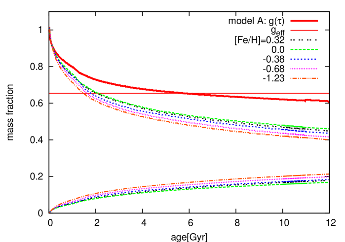
Figure 1: Mass loss due to stellar evolution. The two sets of thin lines show the fractions of luminous mass and of remnants (upper and lower curves, respectively) for the set of metallicities used in the PEGASE code. The full (red) thick line shows the total stellar mass fraction (luminous matter plus remnants) of the fiducial model A taking into account the age-metallicity relation. The overall present day mass fraction of the stars is given by $g_{\mathrm{eff}}$.

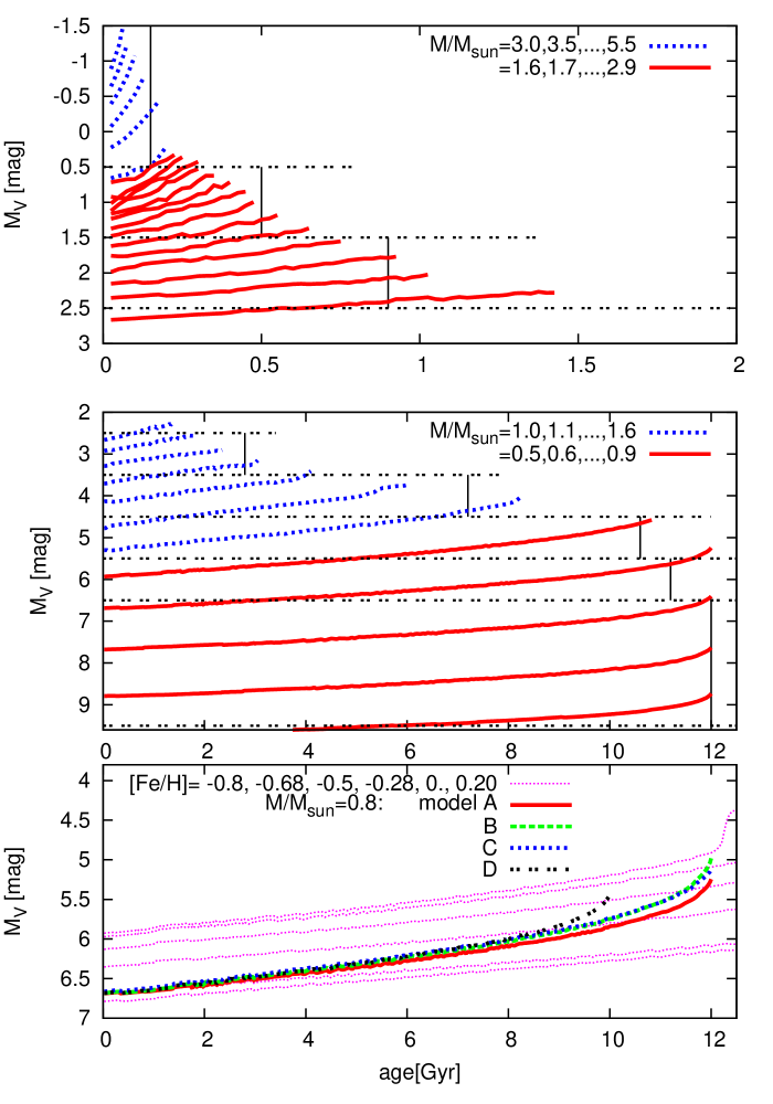
Figure 2: The lower panel shows the age dependence of the absolute luminosity $M_{\mathrm{V}}$ for stars with $M=0.8\,\rm{M}_{\mathrm{\rm\sun}}$ (averaged over $0.1\,\rm{M}_{\mathrm{\rm\sun}}$). Thin lines are the evolution for different metallicities $\mathrm{[Fe/H]}=-0.8;-0.68;-0.5;-0.28;0.0;0.20$ and the thick line shows the present day luminosity of the stars as a function of age taking into account the age-metallicity relation. The upper panels show the luminosity of mass bins along the main sequence as a function of age taking the chemical enrichment into account. Vertical lines give the adopted lifetimes for each luminosity interval.

3 Observational Data

In the model we assume that each stellar sub-population is in dynamical equilibrium in the vertical direction. For the high luminosity end of the main sequence with average age below 1 Gyr this is not guaranteed. On the other hand the observed velocity distribution functions and also the vertical density profile of A stars measured by Holmberg & Flynn (2000) are hints for equilibrium distributions. Additionally we use large radii of 200 pc for these sub-samples and determine a spatially averaged distribution. All sub-samples can be used as independent samples to determine the total vertical gravitational potential $\phi(z)$. The velocity distribution functions $f(|W|)$ of the samples depend on the age distribution of the stars. Therefore we use main sequence stars, where $f(|W|)$ is a function of the lifetime of the stars. In order to determine the vertical velocity distribution function $f(|W|)$ in the solar neighbourhood we need kinematically unbiased samples with space velocities.

For the determination of the AVR we use only the measured velocity dispersions in the magnitude bins along the main sequence using stellar lifetimes. An independent stellar sub-sample are the McCormick K and M dwarfs (Vyssotsky, 1963). Detected by a spectroscopic survey they are free from kinematic bias. Altogether 516 stars show reliable distances - almost all from the Hipparcos Catalogue - and space velocity components. All stars within the 25 pc sphere are also used to determine independently the velocity distribution function $f(|W|)$ of stars with lifetime larger than 12 Gyr (see Fig. 6). For a sub-sample of about 300 stars Wilson & Woolley (1970) estimated the CaII emission intensity at the H and K lines in a relative scale allowing to construct six different age bins under the assumption of a constant SFR (see Jahreiß and Wielen, 1997). For each bin the vertical velocity dispersion is determined. We do not use these sub-samples in our model for two reasons. The determination of the mean ages of the bins are inconsistent with our disc model and for the velocity distribution functions in the age bins the number of stars is too low to obtain reliable $f(|W|)(t)$. The AVR of this sample is shown in the lower panel of Fig. 8 only for comparison.

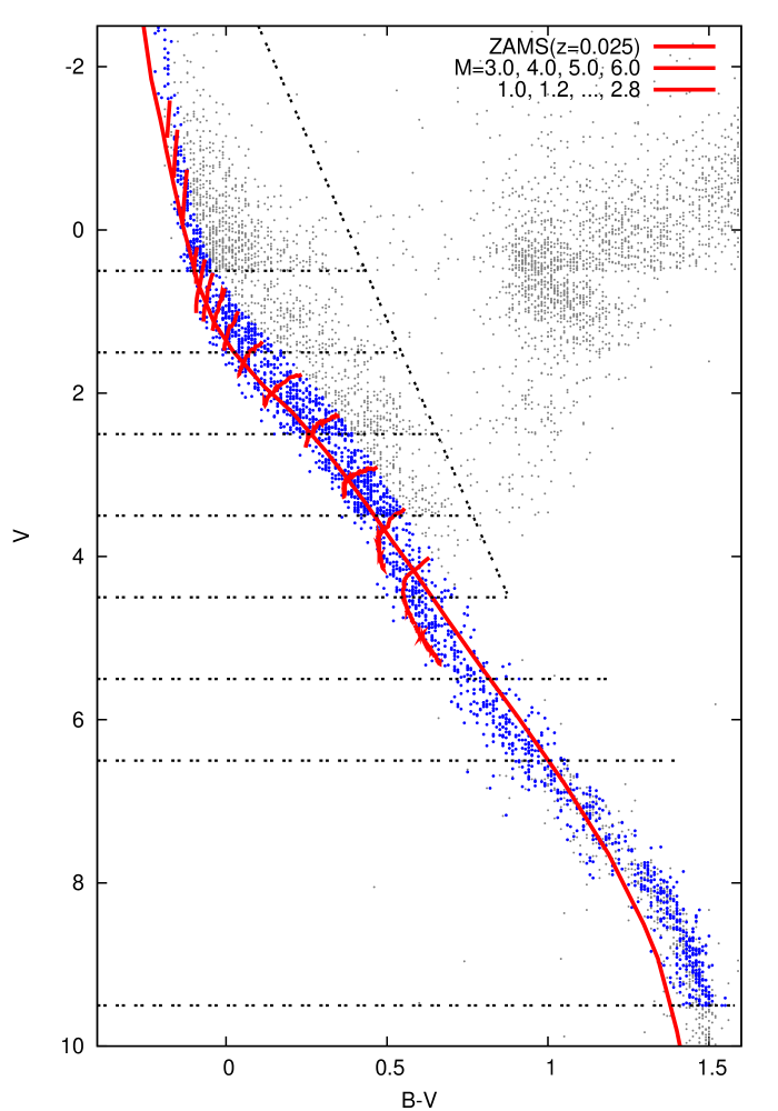
Figure 3: The HR-diagram shows all Hipparcos stars (grey dots) with $\sigma_{\pi}/\pi\leq 0.15$ within the distance limits chosen (see column 3 in Table 1) The selected main sequence stars are over-plotted by larger dark dots. The eight magnitude bins are indicated by the horizontal dotted lines and the inclined line marks the selection including the turnoff stars. The full lines show the ZAMS with present day metallicity and the ’tracks’ from Fig. 2 used for the selection process.

For the determination of $f(|W|)$ along the main sequence we use the Hipparcos stars with good space velocities supplemented at the faint end down to $M_{\mathrm{V}}=9.5$ mag by stars from an updated version of the Catalogue of Nearby stars (CNS4) (Jahreiß & Wielen, 1997), i.e. also most of the CNS4 data rely on Hipparcos results. For the determination of the space velocities good distances, proper motions and radial velocities are required. This was achieved in combining the Hipparcos data with radial velocities originating from an unpublished compilation of the ”best” radial velocities for the nearby stars that was then extended to all Hipparcos stars.

We apply a 2-step selection process. In the first step the absolute visual magnitude $M_{V}$ of the Hipparcos stars was determined from the visual magnitude and the trigonometric parallax given in the Hipparcos catalogue. Only stars with $\sigma_{\pi}/\pi$ smaller than 15% were taken into account. In the case of binaries resolved by Hipparcos the $M_{V}$ of the brighter component was used. It was calculated from the combined magnitude and the magnitude difference measured by Hipparcos. The stellar sample is divided into magnitude bins $M_{\mathrm{V}}=-1\pm 1.5,1\pm 0.5,...,6\pm 0.5,8\pm 1.5$ mag. In order to avoid a kinematic bias we restrict the distances of the stars in each magnitude bin to be well within the completeness limit of the Hipparcos catalogue determined by the magnitude limit $V\sim 7.3$ mag of the Hipparcos Survey. The faintest magnitude bin is restricted to a distance of 25 pc relying on the completeness of the CNS4 (grey dots in Fig. 3).

In the second step we select in the HR-diagram (Fig. 3) a regime along the main sequence in order to exclude most of the turnoff stars as well as all giants and white dwarfs. As zero age main sequence we used the $(B-V,M_{V})$-relation for the present-day metallicity z=0.025 originating from the Padua-isochrones (Bertelli et al., 1994; Girardi et al., 2002) (URL: http://stev.oapd.inaf.it/$\sim$lgirardi/cgi-bin/cmd). Then all stars in the magnitude range $M_{\mathrm{V,ms}}\pm 0.8$ mag were selected. The reason for this additional selection is to match the mass tracks from stellar population synthesis up to the turnoff point described in Sect. 2.5. A selection of these tracks are over-plotted in the HR-diagram. For the brightest magnitude bin the ZAMS is almost vertical and the stars redder than $(B-V)_{ZAMS}+0.10$ were excluded.

This selection is chosen to include the metal-poor MS stars below the ZAMS and to allow for a metallicity scatter of about 0.2dex as well as to include unresolved MS binaries above the single star MS. On the other hand most turnoff stars are excluded, because they would lead to an additional spread of stellar masses and lifetimes in the magnitude bins. For a consistency check we analysed a second set of stellar samples by including the turnoff stars bluer than the inclined line in (Fig. 3) and using the corresponding larger lifetimes derived from stellar evolution. The properties of the resulting samples of main sequence stars are collected in Table 1.

Table 1: Complete samples of nearby main sequence stars: Column 1 lists the source catalogue. Column 2, 3 and 4 list the range in absolute visual magnitude, the selected distance limit, and the total number of stars available, respectively. Column 5 and 6 list the number of stars removed due to poor parallaxes ($\sigma_{\pi}/\pi>.15$) and unknown or poor radial velocities. In column 7 the remaining number of main sequence stars with good space velocity components is given and the last column contains the corresponding number of stars including the turnoff stars.

source	$M_{V}$	$d_{lim}$	N	n∗	no RV	Nfin	$N_{to}$
	[mag]	[pc]
Hip	-2, -1, 0	200	304	39	15	250	931
Hip	1	100	242	0	1	241	497
Hip	2	75	401	8	7	386	650
Hip	3	50	352	0	4	348	491
Hip	4	30	172	2	0	170	194
Hip	5	25	172	0	0	172
Hip	6	25	170	0	2	168
CNS	7, 8, 9	25	525		84	441

For the determination of the velocity distribution functions $f(|W|)$ we correct for the peculiar motion of the Sun using the local standard of rest value $W_{\odot}=7$ km/s given in Delhaye (1965) that is in close agreement to the modern $W_{\odot}=7.17\pm 0.38$ km/s determined by Dehnen & Binney (1998) from the Hipparcos data. The resulting normalised distribution functions are shown in Fig. 6 with a binning of 5 km/s in $|W|$. For the determination of the velocity dispersions we exclude stars with high velocities ($|W|>40\,km/s$ for $M_{\mathrm{V}}<3.5$ and $|W|>60\,km/s$ for $M_{\mathrm{V}}>3.5$).

4 Properties of the disc

We discuss first the algorithm to determine the parameters of best fitting models. Then we describe our fiducial model A in great detail and compare the properties with a selection of other models of similar fitting quality.

4.1 Best fit procedure

The disc model depends on a set of input functions and parameters with strong correlations and degeneracies. Thus a simultaneous best fit of all parameters and an automatic selection of the astrophysical best model is impossible. Therefore it is very useful to sort the input quantities hierarchically by there impact on the velocity distribution functions of MS stars and the structure of the disc.

Figure 4: Flowchart of fitting procedure. For a description see text.

The fitting procedure can be split into three parts: 1) pre-processing to calculate a normalised model; 2) best fit of $f_{\mathrm{i}}(|W|)$ and scaling of the model; 3) post-processing to calculate the output and predictions (see figure 4). We start with a reasonable set of mass fractions $Q_{\mathrm{s,g,t}}$ of the components including the kinematics of the gas, thick disc and DM halo and fix the IMF. From large sets of template functions for the normalised SFR and AVR we select up to ten of each. We select for each SFR a metal enrichment law. Then we construct models for all (SFR,AVR) combinations by calculating the mass loss due to stellar evolution, solving the Poisson equation and determining the local stellar age distribution. With pre-calculated MS lifetimes we determine the normalised velocity distribution functions $f_{\mathrm{i}}(|W|)$ for all nine stellar sub-samples.

In each model we determine the common scaling factor $\sigma_{\mathrm{e}}$ for all $f_{\mathrm{i}}(|W|)$ by a nonlinear Levenberg-Marquardt best fit algorithm (Press et al., 1992). It turned out that a standard $\chi^{2}$ fit is very sensitive to the choice of the velocity range in $|W|$ due to the sparse population in the higher velocity bins. Therefore we tested the $Z^{2}$ statistics from Lucy (2000) which is a modified $\chi^{2}$ statistics leading to a standard distribution also for sparse data sets. This algorithm is very stable and we fix the velocity range to $|W|<40$ km/s for the bright bins with $M_{V}<3.5$ and 60 km/s for the faint bins. For 90 degrees of freedom a reduced $\chi^{2}=1.2$ corresponds to a 10% level of significance that the data are consistent with the model. An inspection of the individual reduced $\chi^{2}$ for the $f_{\mathrm{i}}(|W|)$ shows that the brightest bin with $\chi^{2}>3.0$ is inconsistent with the model on the 99.5% level for all models. This result confirms that these very young stars are not in dynamical equilibrium. Nevertheless we include this bin in our calculation in order not to ignore the low velocity dispersion in that bin. Tests by excluding the first bin and by fitting also the normalisations $n_{\mathrm{i}}$ of the $f_{\mathrm{i}}(|W|)$ does not change the results significantly.

For further investigations we consider only models with $\chi^{2}<1.2$ which already leads to strong constraints in the allowed heating laws AVR. All further iterations are done for individual pairs (SFR,AVR). In the next step the calculated G dwarf metallicity is compared to the observations and a new chemical enrichment law is constructed to give a reasonable fit. Corrections via stellar mass loss and MS lifetimes are small and the new model can be used to derive the conversion factor from the IMF and the local present day mass function (PDMF). Now the IMF can be determined from the observed PDMF which is done in the current phase only for comparison and not iterated.

For the next iteration step we need to scale the model to physical quantities. The first of the two free scaling factors is $\sigma_{\mathrm{e}}$ which is already fixed by the best fit procedure. For the second parameter we decided to fix the local stellar density including the thick disc contribution to $\rho_{\mathrm{s0}}+\rho_{\mathrm{t0}}=0.039\,\rm{M}_{\mathrm{\rm\sun}}\,pc^{-3}$, which is the best observed quantity for the local disc model (Jahreiß & Wielen, 1997). We can rewrite equation 4 to derive $z_{\mathrm{e}}$ by

$$z_{\mathrm{e}}^{2}=\frac{Q_{\mathrm{s}}}{4\pi GC_{\mathrm{eff}}}\frac{\sigma_{\mathrm{e}}^{2}}{\rho_{\mathrm{s0}}} \mathrm{with} C_{\mathrm{eff}}=h_{\mathrm{eff}}/z_{\mathrm{e}}$$ (28)

Then $h_{\mathrm{eff}}$ can be scaled and the total surface density is determined by

$$\Sigma_{\mathrm{tot}}=\frac{2h_{\mathrm{eff}}\rho_{\mathrm{s0}}}{Q_{\mathrm{s}}}$$ (29)

All other quantities can be scaled in a similar way. In this final iteration the input parameters for the surface densities and the kinematics are adapted in such a way as to reproduce the known constraints on surface densities, local densities and scale heights. The thick disc parameters can be freely chosen in a wide range with very little influence on the other disc properties. The kinematic parameters of gas and DM halo are forced to get the correct gas scale height $z_{\mathrm{g}}\sim 100$ pc and DM velocity dispersion $\sigma_{\mathrm{h}}\sim 140$ km/s. The value of $Q_{\mathrm{h}}$ and as a consequence the local halo density $\rho_{\mathrm{h0}}$ are implicitly determined by fixing the other $Q$ values. The value of $Q_{\mathrm{g}}$ is chosen in a simple step to be consistent with the observed surface density of $\Sigma_{\mathrm{g}}\approx 10-13\,\rm{M}_{\mathrm{\rm\sun}}pc^{-2}$ (Dickey & Lockman, 1990). Adapting the thin disc parameter $Q_{\mathrm{s}}$ is more sophisticated, because it has a significant influence on the shape of the gravitational potential. For the boundary conditions we have a relatively large freedom and compare models which fulfil different constraints on the thin disc scale height $z_{\mathrm{s}}$ or on surface densities.

We discuss more details of parameter choice in the next subsections and a more detailed investigation of the best fit procedure and model selection will be given in Paper II.

In the next subsections we discuss the selection of the main input functions SFR and AVR and other properties of the disc models including predictions for future observations.

4.2 Star formation history and dynamical heating

The main input functions that are to be determined, are the SFR and AVR. Since the SFR is a priori not strongly constrained, we start with template sets of smooth functions of different analytic type: pure exponentials with different disc age and decay timescale; linear increase combined with exponential decline; algebraic with linear increase and polynomial decline. For the heating function AVR we use templates of power laws with different power law indices and offsets in time to allow a nonzero present day value. A second set has a constant velocity dispersion for ages larger than 6 or 9 Gyr as proposed by Freeman (1991). A third set of polynomials was chosen to produce an extra flattening or steepening in the AVR around intermediate age of $\sim 6$ Gyr.

In a preliminary study we select those parameter regimes which result in a reasonable $\chi^{2}<1.2$ for at least one heating function AVR. We found that the polynomial functions do not improve the fits for any SFR significantly compared to corresponding power law AVRs. The range of consistent SFRs, based on the local kinematic data alone, is weakly constraint: We find for the present day star formation rate SFR${}_{\mathrm{p}}>1.2\rm{M}_{\mathrm{\rm\sun}}/pc^{2}/Gyr$ (smoothed over the last 500 Myr) and for stars older than 10 Gyr a contribution less than 25%. This means that the overall decline of the SFR is limited to a factor of 4–5.

In the main step we restrict the models further to (SFR,AVR) pairs with $\chi^{2}<1.1$. All models with $\chi^{2}$ below this limit are consistent with the $f_{\mathrm{i}}(|W|)$ of the local MS stars. For each selected SFR the possible AVRs are restricted to at most a few. Since there is still quite a variety of very different models left over, we restricted the further investigation to a representative selection of (SFR,AVR) combinations. The fine-tuning of the model parameters (metal enrichment, gas and DM properties, surface density constraints) is done only for these models. It turned out that these parameter adjustments do not change the best fit significantly (similar $\chi^{2}$ and $\sigma_{\mathrm{e}}$). In the models we fix the surface density of the gas to the observed value and the stellar surface density is determined by the local stellar density and the best fit $\sigma_{\mathrm{e}}$. Therefore the DM surface density, i.e. the mass fraction $Q_{\mathrm{h}}$, is mainly determined by the surface density of all components $\Sigma(|z|<1.1\,kpc)\sim 75\rm{M}_{\mathrm{\rm\sun}}/pc^{2}$ (Kuijken & Gilmore, 1991), (Holmberg & Flynn, 2004). It must be determined by an iteration process, because changing the $Q$’s also changes the scale heights of all components. The second boundary condition is the scale height $z_{\mathrm{s}}$ of the thin disc. It is connected to $Q_{\mathrm{s}}$ via the scaling length $z_{\mathrm{e}}$ (equation 28). The standard value of 325$\pm$50 pc determined by Bahcall & Soneira (1984) from star counts is still reliable and widely used. Since this scale height is calculated from a one component exponential thin disc, it corresponds to the mean exponential falloff in the range of $|z|\sim 100-1000$ pc which is much closer to the mid-plane than our value $z_{\mathrm{s}}$ measuring the exponential scale height in the range $|z|\sim 600-1500$ pc. An inspection of the density profile shapes (figure 11) shows that closer to the mid-plane the local scale height is $\sim$20% larger than $z_{\mathrm{s}}$. Therefore we try to reach in the models $z_{\mathrm{s}}\sim 270-300$ pc which is not possible in all cases. Reducing the DM fraction increases the thin disc fraction $Q_{\mathrm{s}}$ and as a consequence the scale height $z_{\mathrm{s}}$. As a bottom line there is a trade-off to reach both constraints given by $\Sigma(|z|<1.1\,\mathrm{kpc})$ and $z_{\mathrm{s}}$. A general overview over all models and a detailed discussion of the parameter dependence will be given in Paper II (Just & Jahreiß, 2009).

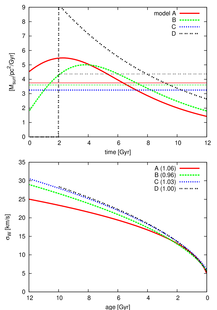
Figure 5: The upper panel shows the SFRs of models A–D. The horizontal lines are the corresponding mean values $\langle\mathrm{SFR}\rangle\,$. The lower panel gives the AVRs of models A–D($\chi^{2}$ values in parentheses). Age is running backwards.

We present four models A–D with very different SFR. For clarity we use model A as the fiducial model that will be described in great detail. The SFR of this model is very close to that investigated also by Aumer & Binney (2009). We discuss the similarities and differences of models B–D with respect to model A. The data of models E–G are added to show the effect of some parameter variations. The basic properties of the models are

Model A:

Fiducial model with maximum SFR 10 Gyr ago and mass fractions chosen to get simultaneously a small thin disc scale height of $\sim 270$ pc and a surface density $\Sigma(|z|<1.1\,kpc)\sim 75\rm{M}_{\mathrm{\rm\sun}}/pc^{2}$.

Model B:

Model with smallest reduced $\chi^{2}=0.96$ of all models; optimised as model A

Model C:

Model with constant SFR; DM fraction increased to the upper limit in order to get a reasonable thin disc scale height of $z_{\mathrm{s}}\sim 300$ pc

Model D:

Model with reduced disc age of $t_{\mathrm{p}}=10$ Gyr and exponential SFR with shortest consistent decline timescale.

Model E:

Model with same SFR, AVR as model A but neglecting the thick disc component.

Model F:

Like model A but with larger local stellar density.

Model G:

Like model F but with larger gas fraction in order to increase the local density further.

The SFRs and AVRs of models A–D are shown in figure 5 together with the mean SFR determined by $\langle SFR\rangle\,=S_{0}/t_{\mathrm{p}}$. A list of model parameters and derived physical quantities discussed in this paper is given in Table 2 together with the corresponding data of other authors.

Table 2: Disc properties for models A–G and some models from the literature. Global parameters: $\chi^{2}$ value of the fit; maximum height $z_{\mathrm{max}}$, local density$\rho_{\mathrm{0}}$, surface densities below 0.35 and 1.1 kpc, total surface density of the disc. Thin disc properties: maximum velocity dispersion $\sigma_{\mathrm{e}}$, mean and present day SFR, local density $\rho_{\mathrm{s0}}$; surface density $\Sigma_{\mathrm{s}}$ up to $z_{\mathrm{max}}$, (half-)thickness $h_{\mathrm{eff}}$, exponential scale height $z_{\mathrm{s}}$; Thick disc properties: velocity dispersion $\sigma_{\mathrm{t}}$, local density $\rho_{\mathrm{t0}}$; surface density $\Sigma_{\mathrm{t}}$ up to $z_{\mathrm{max}}$, exponential scale height $z_{\mathrm{t}}$; power law index $\alpha_{\mathrm{t}}$ of sech${}^{\alpha_{\mathrm{t}}}$ fit. Gas component: local density $\rho_{\mathrm{g0}}$; surface density $\Sigma_{\mathrm{g}}$ up to $z_{\mathrm{max}}$, (half-)thickness $h_{\mathrm{eff,g}}$; exponential scale heights $z_{\mathrm{g}}$; DM halo: velocity dispersion $\sigma_{\mathrm{h}}$, local density $\rho_{\mathrm{h0}}$; surface density $\Sigma_{\mathrm{h}}$ up to $z_{\mathrm{max}}$.

quantity	unit	A	B	C	D	E	F	G	other sources
		fiducial	min.$\chi^{2}$	const.SFR	lt.=10Gyr	no.thick d.	larger $\rho_{s0}$	more gas
red. $\chi^{2}$	-	1.057	0.960	1.025	0.994	1.046	1.056	1.054
$z_{\mathrm{max}}$	kpc	2.3	2.7	2.7	3.1	2.3	2.3	2.3
$\rho_{\mathrm{0}}$	$\rm{M}_{\mathrm{\rm\sun}}/pc^{3}$	0.088	0.091	0.092	0.092	0.088	0.094	0.101	0.0761, 0.0982
$\Sigma(<0.35)$	$\rm{M}_{\mathrm{\rm\sun}}/pc^{2}$	41.1	41.3	42.3	40.7	41.0	43.5	44.5	413
$\Sigma(<1.1)$	”	73.5	73.2	79.3	71.8	72.5	74.9	74.5	74$\pm 6^{3}$, 71$\pm 6^{4}$
$\Sigma_{\mathrm{disc}}$	”	45.2	45.7	42.1	46.7	41.8	49.2	50.4	56$\pm 6^{3}$, 48$\pm 9^{4}$
$\langle SFR\rangle$	$\rm{M}_{\mathrm{\rm\sun}}/pc^{2}/Gyr$	3.75	3.60	3.25	4.38	3.99	4.09	4.02
SFRp	”	1.43	1.80	3.33	2.20	1.55	1.58	1.42
$\sigma_{\mathrm{e}}$	km/s	25.0	28.4	29.9	28.0	25.1	25.0	25.1	17.51
$\rho_{\mathrm{s0}}$	$\rm{M}_{\mathrm{\rm\sun}}/pc^{3}$	0.037	0.037	0.037	0.037	0.039	0.041	0.041	0.0451, 0.0442
$\Sigma_{\mathrm{s}}$	$\rm{M}_{\mathrm{\rm\sun}}/pc^{2}$	29.4	28.6	26.3	29.2	31.4	32.1	31.6	34.42
$h_{\mathrm{eff}}$	pc	400	389	357	398	402	386	379
$z_{\mathrm{s}}$	”	274	295	303	309	277	266	265
$\sigma_{\mathrm{t}}$	km/s	45.1	45.4	44.9	44.9	-	45.1	45.1	373
$\rho_{\mathrm{t0}}$	$\rm{M}_{\mathrm{\rm\sun}}/pc^{3}$	0.0022	0.0023	0.0022	0.0023	-	0.0025	0.0024	0.0073
$\Sigma_{\mathrm{t}}$	$\rm{M}_{\mathrm{\rm\sun}}/pc^{2}$	5.3	5.7	5.4	5.8	-	5.7	5.6
$z_{\mathrm{t}}$	pc	793	807	680	815	-	808	827
$\alpha_{\mathrm{t}}$	-	-1.19	-1.17	-1.60	-1.13	-	-1.07	-1.00
$\rho_{\mathrm{g0}}$	$\rm{M}_{\mathrm{\rm\sun}}/pc^{3}$	0.035	0.038	0.035	0.040	0.034	0.037	0.042	0.0211, 0.0502
$\Sigma_{\mathrm{g}}$	$\rm{M}_{\mathrm{\rm\sun}}/pc^{2}$	10.5	11.4	10.5	11.7	10.5	11.4	13.2	61, 132
$h_{\mathrm{eff,g}}$	pc	151	149	151	145	151	152	148	1401
$z_{\mathrm{g}}$	”	94	98	98	97	94	96	94	1401
$\sigma_{\mathrm{h}}$	km/s	140	141	141	141	141	140	140	851
$\rho_{\mathrm{h0}}$	$\rm{M}_{\mathrm{\rm\sun}}/pc^{3}$	0.014	0.014	0.018	0.013	0.015	0.013	0.012	0.011
$\Sigma_{\mathrm{h}}$	$\rm{M}_{\mathrm{\rm\sun}}/pc^{2}$	59.9	68.6	89.4	70.1	62.7	54.4	51.4

¹ Robin et al. (2003); ² Holmberg & Flynn (2000); ³ Holmberg & Flynn (2004); ⁴ Kuijken & Gilmore (1991)

For models A–D we give explicitly the input functions to allow the reader to make comparison calculations. We find for models A and B

$$\mathrm{SFR}(t) = \langle\mathrm{SFR}\rangle\,\frac{(t+t_{0})t_{n}^{3}}{(t^{2}+t_{1}^{2})^{2}}\quad\mathrm{with}$$ (30)

$$A : \,t_{0}=5.6\,\mathrm{Gyr}\,;\,t_{1}=8.2\,\mathrm{Gyr}\,;\,t_{n}=9.9\,\mathrm{Gyr}$$

$$B : \,t_{0}=1.13\,\mathrm{Gyr}\,;\,t_{1}=7.8\,\mathrm{Gyr}\,;\,t_{n}=11.7\,\mathrm{Gyr}\,,$$

for model C

$$\mathrm{SFR}(t) = \langle\mathrm{SFR}\rangle$$ (31)

and for model D

$$\mathrm{SFR}(t) = \langle\mathrm{SFR}\rangle\,\frac{t_{\mathrm{p}}}{t_{\mathrm{e}}}\frac{\exp(-t/t_{\mathrm{e}})}{1-\exp(-t_{\mathrm{p}}/t_{\mathrm{e}})}$$ (32)

$$D : \,t_{\mathrm{e}}=8\,\mathrm{Gyr}\,;\,t_{\mathrm{p}}=10\,\mathrm{Gyr}\,.$$

For the dynamical heating function AVR we use a power law

$$\sigma_{\mathrm{W}}(\tau) = \sigma_{\mathrm{e}}\left(\frac{\tau+\tau_{0}}{t_{\mathrm{p}}+\tau_{0}}\right)^{\alpha}\quad\mathrm{with}$$ (33)

$$A : \,\alpha=0.375\,;\,\tau_{0}=0.17\,\mathrm{Gyr}\,;\,t_{\mathrm{p}}=12\,\mathrm{Gyr}\,$$

$$B : \,\alpha=0.5\,;\,\tau_{0}=0.5\,\mathrm{Gyr}\,;\,t_{\mathrm{p}}=12\,\mathrm{Gyr}\,$$

$$C : \,\alpha=0.5\,;\,\tau_{0}=0.5\,\mathrm{Gyr}\,;\,t_{\mathrm{p}}=12\,\mathrm{Gyr}\,$$

$$D : \,\alpha=0.5\,;\,\tau_{0}=0.32\,\mathrm{Gyr}\,;\,t_{\mathrm{p}}=10\,\mathrm{Gyr}\,.$$

Model C with constant SFR is of special interest, because it is still used in many applications directly or implicitly. Model C fits well the local kinematic data. Due to the large fraction of young and dynamically cool stars a larger initial velocity dispersion and a higher fraction of DM matter is needed. The relatively large values for $\Sigma(|z|<1.1\,\mathrm{kpc})$ and $z_{\mathrm{s}}$ are still within the limits.

4.3 Kinematics of the disc

All presented models show reasonable fits to the set of normalised velocity distribution functions $f_{\mathrm{i}}(|W|)$ for the nine samples of MS stars described in section 3, because the total reduced $\chi^{2}<1.1$. For models A–D the total $\chi^{2}$ values are given in the lower panel of figure 5. In figure 6 the data are compared to model A in all samples. For comparison in each column one of the other models B–D are shown. We also computed the $\chi^{2}_{\mathrm{i}}$ of the individual distribution functions $f_{\mathrm{i}}(|W|)$ to check the individual contributions. The values are given in parentheses in figure 6. The distribution of the $\chi^{2}_{\mathrm{i}}$ are consistent with a random distribution with one exception. In all models the brightest bin has an individual reduced $\chi_{\mathrm{1}}^{2}>3$ for eight degrees of freedom (= number of bins). The inset in the upper left panel of figure 6 shows the the distribution function of models A–D in log-scale for the bins between 10 and 20 km/s, where the significant deviations occur. The $1-\sigma$ standard Poisson noise of the data (shown by the errorbars) are not a precise measure of the contribution to $\chi^{2}$, since we use the $Z^{2}$ statistics (for details see Paper II). This is a hint to a significant departure from the assumed equilibrium distribution. This is not surprising, since the lifetime of these stars is of the order of the vertical oscillation frequency in the disc and dynamical equilibrium cannot be achieved in this short time. In Fig. 7 we show for model A that the distribution functions $f(|W|)$ including the turnoff stars agree just as well with the theoretical distribution functions using the appropriate lifetimes.

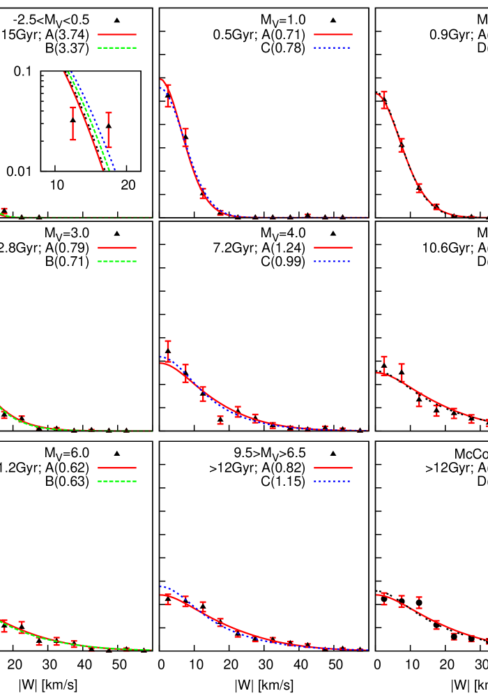
Figure 6: The normalised velocity distribution functions $f_{\mathrm{i}}(|W|)$ for the different sub-samples given in Table 1 and for the McCormick stars (lower right). Symbols are the data and full lines represent the fiducial model A. In each column the distribution functions of one of the comparison models are added: B: best $\chi^{2}$; C: const. SFR; D: exp.SFR and lifetime=10 Gyr. The inset in the upper left panel shows the part of $f_{\mathrm{i}}(|W|)$ (in log-scale), where the significant deviations occur.

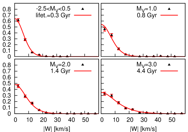
Figure 7: The normalised velocity distribution functions $f(|W|)$ of the four brightest bins as in Fig. 6 but with turnoff stars included.

The AVR can be observed only by kinematically unbiased stellar sub-samples with direct age determinations. In the lower panel of figure 8 the AVRs of the models A–D are reproduced from figure 5 in log-scale and compared to two data sets. The circles are the McCormick K and M dwarfs with ages determined from H and K line strength (Jahreiß & Wielen, 1997) and the asterisks represent the F and G stars of GCS2 with good age determinations. The ages of the McCormick stars were derived by adopting a constant SFR and should therefore be consistent with model C. Corrections for a declining SFR as in the other models would shift the mean ages of the bins systematically to higher values. It is interesting to note that the best AVR for models B and C are the same. The best fit scaling $\sigma_{\mathrm{e}}$ is different. This shows that the variation of the SFR has only a small influence on the shape of the AVR.

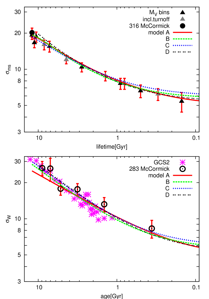
Figure 8: Upper panel: The symbols show the velocity dispersion of the stars along the main sequence (magnitude bins) as a function of mean lifetime determined from stellar evolution (Fig. 2). The full line gives the result of the fiducial model A. The other lines are for the comparison models B–D. Lower panel: The lines show the velocity dispersion as a function of age (AVR) for the stellar sub-populations of the models. Full symbols are the age groups of the McCormick K and M dwarfs (Jahreiß & Wielen, 1997) and the asterisks are from GCS2.

The velocity dispersions of the sub-samples of MS stars with no age subdivision are determined by the weighted mean over the lifetime with the local age distribution.

For the AVRs of the different models we find power laws with indices $0.375<\alpha<0.5$. This is in the range of the classical value of 0.5 (Wielen, 1977), of 0.53 (Holmberg et al., 2009), and of 0.45 derived by Aumer & Binney (2009). The best fit slope depends strongly on the zero point for newly born stars. A higher initial velocity dispersion $\sigma_{\mathrm{W,0}}$ leads to a shallower heating function described by a larger power law index. All our models require a large $\sigma_{\mathrm{W,0}}$ and a steep rise of the AVR to reproduce the distribution functions of stars with lifetimes 0.5-3 Gyr. The maximum velocity dispersion of the oldest thin disc stars is 25-30 km/s dependent on the SFR.

The upper panel of Fig. 8 shows the excellent agreement of the model with the data from the nearby stars. The black triangles are the velocity dispersions in the magnitude bins of the main sequence stars with lifetimes from Fig.  2. The full circle is the velocity dispersion of the McCormick stars. The underlying distribution functions of these data sets were used for the best fitting. The grey triangles are the velocity dispersions including the turnoff stars in the five magnitude bins with $M_{V}<4.5$ mag. As expected, they show a systematically larger velocity dispersion and have larger lifetimes compared to the pure MS samples. These data confirm the underlying assumption of a continuous disc heating and dynamical equilibrium of the stellar sub-samples.

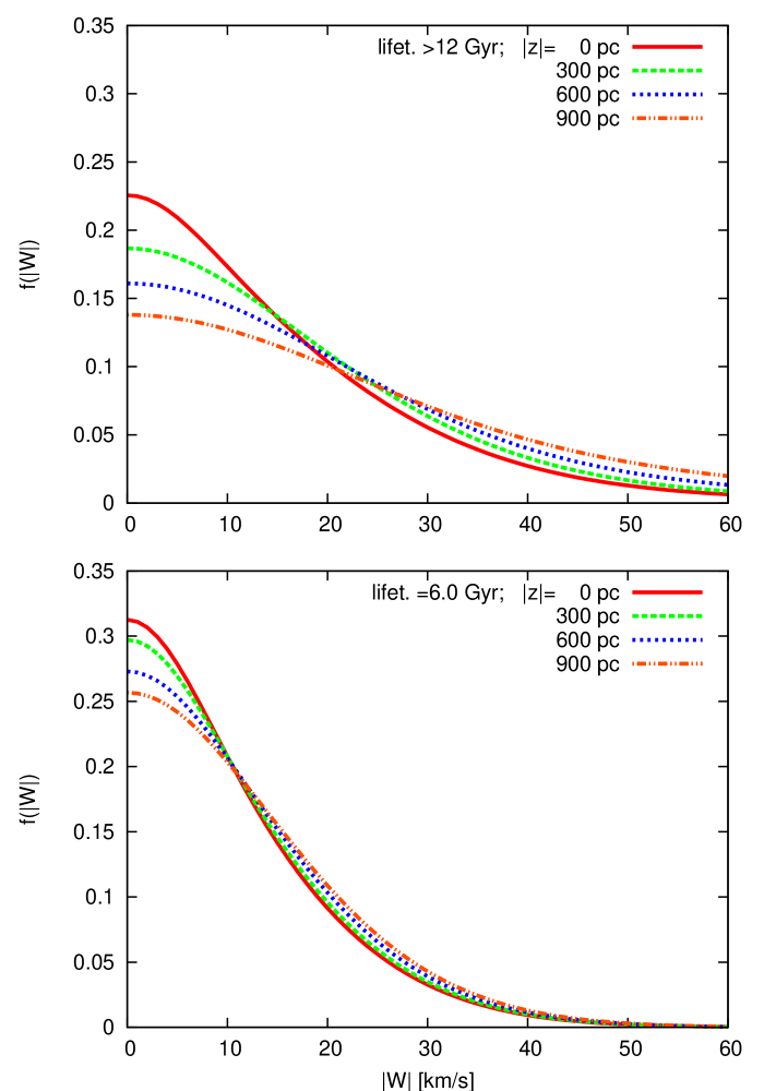
Figure 9: The normalised velocity distribution functions $f(|W|)$ (for $dw=5$ km/s) at different heights $z$ for model A. The upper panel shows of stars with lifetimes larger than 12 Gyr including the thick disc contribution, whereas the lower panel is for thin disc stars with lifetime 6.0 Gyr.

Since the shape of $f(|W|)$ depends on the age distribution of the stars, it depends also on the height $z$ above the mid-plane. Fig. 9 shows the variation above the plane for stars with lifetimes larger than 12 Gyr (upper panel) and stars with a lifetime of 6 Gyr (lower panel; corresponding to magnitudes $M_{\mathrm{V}}=3.5-4$ mag). The vertical gradient in the velocity dispersion of all thin disc stars is slightly stronger than that of the stars with lifetimes larger than 12 Gyr, because the dip near the mid-plane is enhanced due to the contribution of stars with smaller lifetimes. The profile is shown in figure 10 for models A and C. The large fraction of young stars in model C with constant SFR leads to a significantly larger gradient.

4.4 Density profiles

The shape of the vertical density profiles of all components and sub-populations are determined by their kinematics and the self-consistent gravitational potential. A general feature of the vertical density profiles of the stars and of the gas is the flattening at the galactic plane. All profiles are between an exponential profile and that of an isolated isothermal profile given by a sech² function. In the upper panel of figure 10 the profiles of model A are shown. The stellar disc profile of model C (also plotted in figure 10) is significantly flatter and deviates from model A in the regime $|z|\sim 500$ pc and above $|z|\sim 1500$ pc. The second plot in figure 10 shows the difference in the $K_{\mathrm{z}}$ force that is a measure of the total surface density up to $|z|$, of models A and C. Below 500 pc the profiles are very similar despite the differences in the mass fractions and the kinematics. The corresponding surface density values of Kuijken & Gilmore (1991) and Holmberg & Flynn (2004) are added.

For the gas, the thickness is $\sim$150 pc compared to the exponential scale height of $\sim$100 pc. The density profile and the surface density are consistent with the observed HI-profile (Dickey & Lockman, 1990): 0.014 $\rm{M}_{\mathrm{\rm\sun}}/\mathrm{pc}^{3}$, 5.0 $\rm{M}_{\mathrm{\rm\sun}}/\mathrm{pc}^{2}$, 177 pc for the mid-plane density, surface density, thickness) adding about 50% of H₂ with smaller scale height (Bronfman et al., 1988) and applying the correction factor of 1.4 for Helium and heavy elements.

Due to the gravitational potential of the disc, the local density of the dark matter halo is $\sim$50% larger than the DM density at $z_{\mathrm{max}}$ and $\sim$20% larger than the mean DM density given by $\Sigma_{\mathrm{h}}/(2z_{\mathrm{max}})$.

A measure of the profile flattening is given by the ratio of the thickness and the exponential scale height. The half-thickness of MS stars $h_{\mathrm{ms}}$ as function of lifetime is shown in the lower panel of Fig. 12 for all models A–D. The differences above a lifetime of 6 Gyr is significant leading to differences in the determination of surface densities from local densities as used in the estimation of the SFR and IMF from local data. For model A additionally the exponential scale height $z_{\mathrm{exp}}$ as function of lifetime and the half-thickness $h_{\mathrm{age}}$ as function of age are plotted. For young populations $z_{\mathrm{exp}}$ is much smaller than $h_{\mathrm{ms}}$, because the density profiles have Gaussian and not exponential wings. For longer lifetimes $h_{\mathrm{ms}}$ is $\sim$50% larger than $z_{\mathrm{exp}}$.

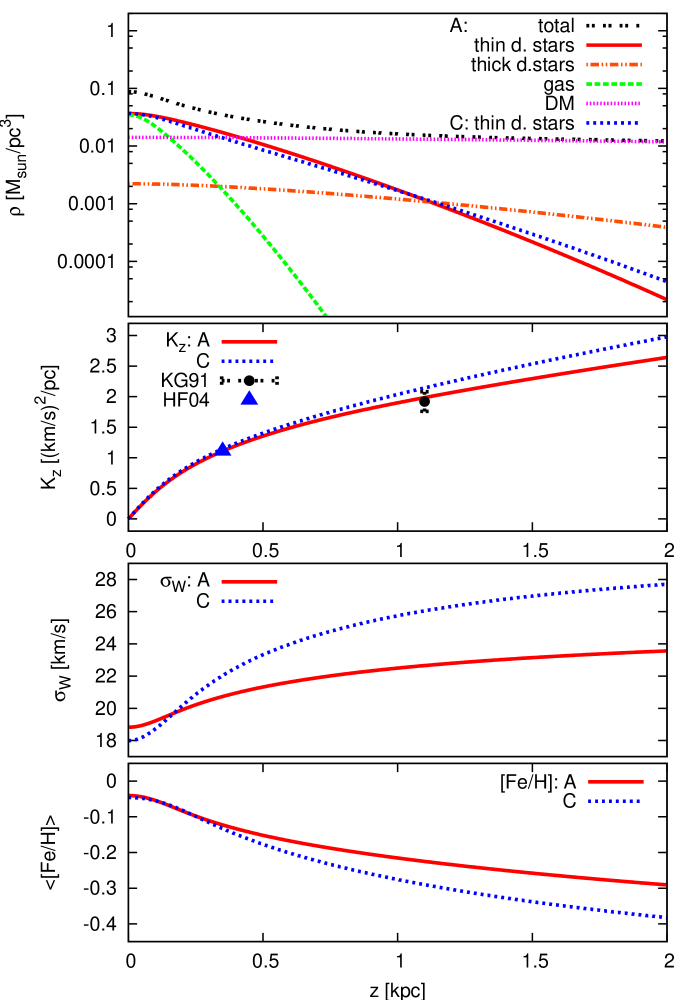
Figure 10: Vertical profiles of the model A and of the thin disc of model C (SFR=const.). From top to bottom: Density profiles; $K_{\mathrm{z}}$ force complemented by the corresponding surface densities of Kuijken & Gilmore (1991) and Holmberg & Flynn (2004); velocity dispersion of the thin stellar disc; V-band luminosity weighted mean metallicity of the thin stellar disc.

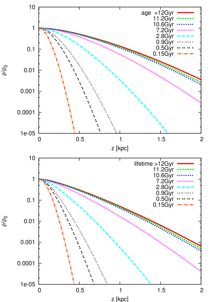
Figure 11: Upper panel: Normalised density profiles of the stellar sub-populations as a function of age. Lower panel: Same for the main sequence stars as a function of lifetime. The set of lifetimes corresponds to the mean lifetimes of the sub-samples used for the velocity distribution functions (see Fig. 6).

The density profiles of MS stars differ in shape from the profiles of the sub-populations of single ages. The lower panel of Fig. 11 shows the normalised density profiles with lifetimes according to the samples used for the model. They are steeper than the corresponding profiles of the sub-populations with the same age and significantly shallower than the density profile using the mean age of the sub-population. This difference is quantified by the thicknesses $h_{\mathrm{age}}$ and $h_{\mathrm{ms}}$ shown in the lower panel of Fig. 12.

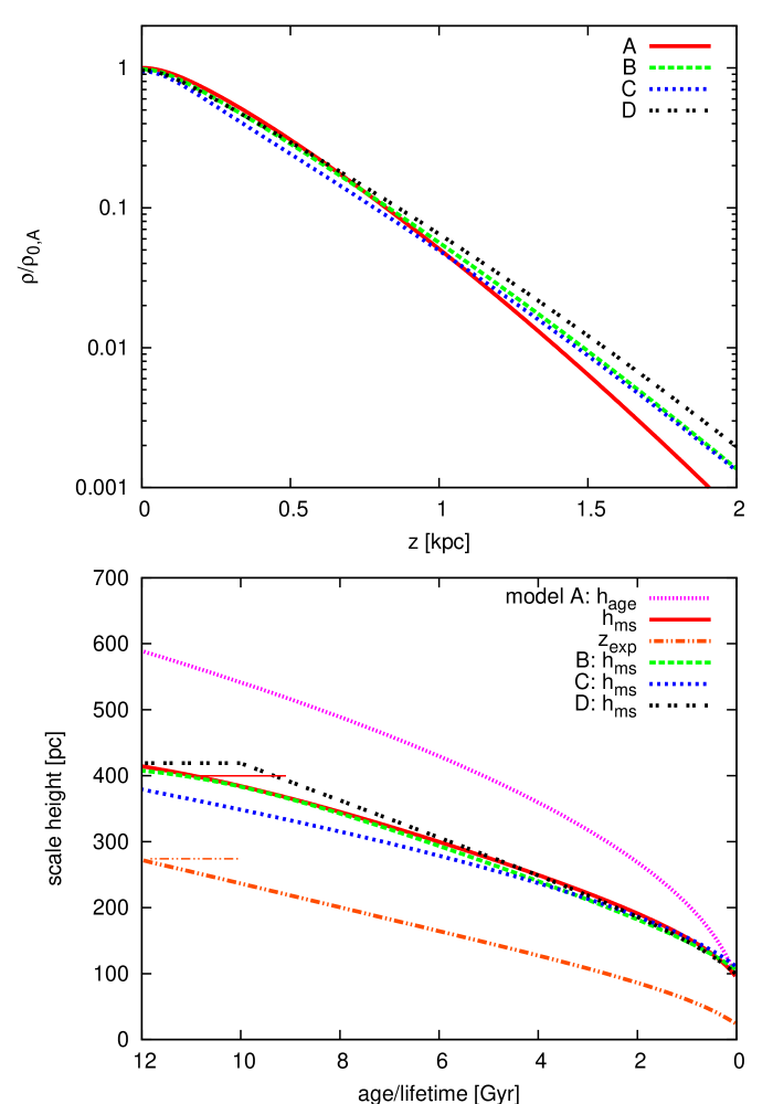
Figure 12: Top panel: Comparison of the density profiles for thin disc stars with lifetimes larger than the age of the disc. Bottom panel: The (half-)thickness of the sub-populations as a function of age $h_{\mathrm{age}}$ and of the MS stars as a function of lifetime $h_{\mathrm{ms}}$. For comparison the exponential scale heights $z_{\mathrm{exp}}$ for the MS stars are included. The horizontal lines are the overall thickness $h_{\mathrm{eff}}$ and the exponential scale height $z_{\mathrm{s}}$ of all stars.

An independent test of the model is the comparison with directly observed density profiles of MS stars as derived by Holmberg & Flynn (2000) for two sub-samples of A stars (with $0<M_{V}<1$ mag) and early F stars (with $1<M_{V}<2.5$ mag). The mean stellar lifetime in these magnitude bins are 0.3 Gyr and 1.0 Gyr, respectively, including turnoff stars. In order to minimise the systematic asymmetry of the profiles (mainly for the A stars) we applied an additional offset of the solar position in $z$ of +5 pc. The result is shown in figure 13. For the A stars all profiles are shifted by a factor of two to avoid overlaps. Over-plotted are the normalised profiles of models A–D and F,G. The observed profile for the F stars is in very good agreement with all models. The observed profile of the A stars is slightly steeper than the model and requires a larger local density or an even shorter lifetime. Models F and G show the effect of a larger local density in two steps (see table 2). Since we do not expect that these stars are already in dynamical equilibrium, the deviations are in a reasonable range.

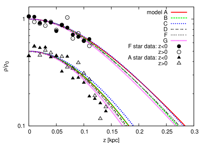
Figure 13: Density profiles for the A and F star sample from Holmberg & Flynn (2000) with an arbitrary vertical offset (full and open symbols below and above the mid-plane, respectively. The lines are models A–D and F,G for corresponding mean lifetimes 0.4 Gyr and 1.0 Gyr for the A and F stars, respectively. The profiles for the A stars are shifted additionally by a factor of two.

In the Besançon model (Robin et al., 2003) Einasto laws are used for the density distribution of isothermal sub-populations. The thicknesses (=flattening in their model) are determined by solving the Poisson equation. The shapes of the density profiles deviate systematically from our results and this means that dynamical equilibrium is achieved only approximately. A detailed investigation of the differences to our model is beyond the scope of this paper.

4.5 Age distributions

The age distributions of the stellar sub-samples of MS stars depend on the lifetime and on the vertical structure. The upper panel of figure 14 shows for model A the normalised local age distribution for different lifetimes. The comparison with the SFR shows clearly the over-representation of young stars in the solar neighbourhood due to the increasing thickness with age. The vertical dilution is quantified by the (half-)thickness $h_{\mathrm{ms}}$ (lower panel of Fig. 12).

A comparison of the local age distributions of stars with lifetime larger than the age of the disc for models A–D are shown in the lower panel of figure 14. In model A the local age distribution of stars with lifetime larger than the disc age varies by less than a factor of two around the mean value. Binney et al. (2000) and Cignoni et al. (2006) propose a constant local age distribution in this sense. This is consistent with our model taking the uncertainties of isochrone ages into account. In model B there is a lack of old stars which cannot be tested by direct measurements, because for this age range the age determinations are very uncertain. Model C with constant SFR predicts a strong dominance of young stars in contrast to the findings of Binney et al. (2000) and Cignoni et al. (2006).

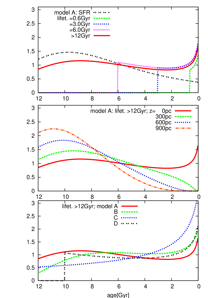
Figure 14: The upper panel shows the normalised local age distributions of MS stars with different lifetimes. The middle panel shows the age distribution of stars with lifetime larger than 12 Gyr at different heights above the Galactic plane. The lower panel shows the local age distributions of models A–D.

The age distributions are a strong function of $z$ above the plane. The middle panel of Fig. 14 shows the lack of young stars in steps of $\Delta z=300$ pc above the mid-plane.

4.6 Metallicity

Since MS luminosities and lifetimes depend on metallicity, we include a simple analytic metal enrichment law $\mathrm{[Fe/H]}(t)$. We adopt a generalised form of a closed box model with a Schmidt star formation law for the oxygen abundance [O/H]$(t)$ (Just et al., 1996) and transform it by a linear approximation to [Fe/H] from Reddy et al. (1993) for thin disc stars, i.e.

$$\mathrm{[Fe/H]}(t) = 2.67\mathrm{[O/H]}(t)$$

$$\mathrm{[O/H](t)} = \lg\left(Z_{\mathrm{oxy}}(t)\right)$$ (34)

$$Z_{\mathrm{oxy}}(t) = Z_{\mathrm{oxy,0}}+\left(Z_{\mathrm{oxy,p}}-Z_{\mathrm{oxy,p}}\right)\frac{\lg\left[1+\ln(1+q\,(t/t_{\mathrm{p}})^{r}\right]}{\ln(1+q)}$$

There are four fitting parameters $q,r,\mathrm{[Fe/H]}_{0},\mathrm{[Fe/H]}_{\mathrm{p}}$ which determine the scaling and the curvature. We tested a large range of parameters: initial metallicity $\mathrm{[Fe/H]}_{0}$=-0.6…-0.8, present day metallicity $\mathrm{[Fe/H]}_{\mathrm{p}}$=-0.1…+0.2, linear increase up to steep early enrichment covering $\mathrm{[Fe/H]}$=-0.4…+0.1 at an age of 6 Gyr. In order to reproduce the high metallicity tail without intrinsic scatter we investigated also some AMRs with an additional accelerated enrichment in the last 2 Gyr. In every case it turned out that the local G dwarf metallicity distribution is a strong restriction for the AMR for any given SFR and AVR. The parameters for models A–D are

$$A : q=2\,;\,r=0.55\,;\,\mathrm{[Fe/H]}_{0}=-0.6\,;\,\mathrm{[Fe/H]}_{\mathrm{p}}=0.02$$

$$B : q=2\,;\,r=0.55\,;\,\mathrm{[Fe/H]}_{0}=-0.8\,;\,\mathrm{[Fe/H]}_{\mathrm{p}}=0.01$$

$$C : q=3\,;\,r=0.70\,;\,\mathrm{[Fe/H]}_{0}=-0.67\,;\,\mathrm{[Fe/H]}_{\mathrm{p}}=-0.01$$

$$D : q=2\,;\,r=0.55\,;\,\mathrm{[Fe/H]}_{0}=-0.6\,;\,\mathrm{[Fe/H]}_{\mathrm{p}}=0.01$$

The metal enrichment laws are shown in the lower panel of figure 16. For model A [O/H] is also plotted. The local metallicity distribution is very sensitive to the present day metallicity due to the shallow slope.

From the metal enrichment the local metallicity distribution for stars with lifetime larger than the age of the disc is calculated. Before binning the theoretical distribution we add a Gaussian scatter which represents an intrinsic scatter and observational errors. We tested a range up to 0.2 dex and found a best value of 0.13 dex corresponding to a FWHM=0.31 dex in order to reproduce both the narrow width of the maximum and the high metallicity wing in the observations (see figure 15). The local metallicity distribution is determined from the Copenhagen F and G star sample (Nordström et al., 2004) selecting all stars with masses $0.84\leq M/\rm{M}_{\mathrm{\rm\sun}}\leq 0.90$ up to the completeness limit $r<40$ pc. The lower mass limit of $0.84\rm{M}_{\mathrm{\rm\sun}}$ was chosen in order to avoid incompleteness for the less luminous metal rich stars. The upper limit was set to be consistent with a lifetime larger than 12 Gyr for the selected stars.

For model A the comparison of the derived local metallicity distribution for stars with adopted lifetime larger than 12 Gyr and the data of the selected mass bin is shown in the upper panel of Fig. 15. The results for models B–D are very similar. The middle panel of Fig. 15 shows the predicted metallicity distribution in model A for stars with lifetime 6 Gyr compared to the observed distribution with lifetime larger than 12 Gyr in the solar neighbourhood. The lower panel shows the same comparison but at $|z|=900$ pc.

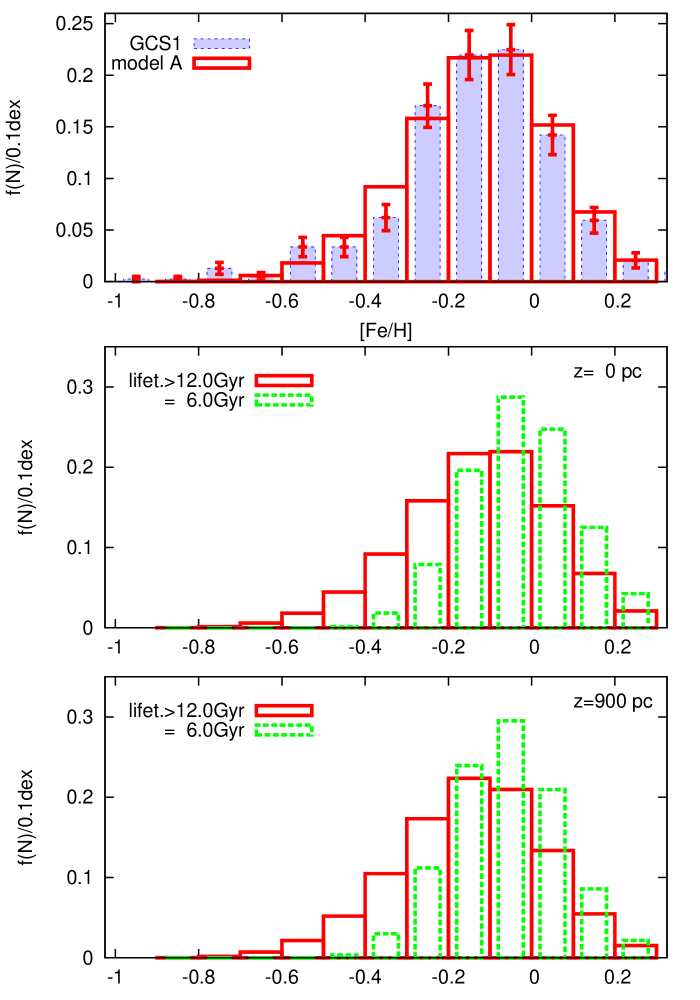
Figure 15: Upper panel: The metallicity distribution of model A compared to the observations from GCS1 in the stellar mass range $0.84\leq M/\rm{M}_{\mathrm{\rm\sun}}\leq 0.90$. Lower panels: The metallicity distribution for dwarfs with lifetime 6.0 Gyr in comparison to the dwarfs with lifetime $>12$ Gyr in the solar neighbourhood and 900 pc above the mid-plane.

The metal enrichment [O/H] and the SFR can be embedded in a local chemical evolution model with primordial gas infall. Since the gas infall rate is an additional free function, the metal enrichment cannot be derived directly from the SFR, IMF and stellar yields. We proceed in the following way. For the oxygen enrichment we adopt instantaneous recycling and mixing to determine the infall rate of primordial gas. The mass loss from stellar evolution is taken into account. Then the oxygen yield in solar units is given by

$$Y_{\mathrm{oxy}}=\langle Z_{\mathrm{oxy}}\rangle+Z_{\mathrm{oxy,p}}\frac{\Sigma_{\mathrm{g}}}{S_{0}}+Z_{\mathrm{oxy,0}}\frac{G_{0}}{S_{0}}$$ (35)

Here $\langle Z_{\mathrm{oxy}}\rangle$ is the mean metallicity of all born stars (not in log-scale and weighted by mass), $G_{0}$ is the initial surface density of gas, $\Sigma_{\mathrm{g}}$ the present day value and $S_{0}$ the total amount of born stars. We start with a negligible initial amount of gas $G_{0}$ and find for the yields in solar units of models A–D $y_{\mathrm{oxy}}=1.1135,1.1301,1.1290,1.1350$, respectively. The infall rate, the surface density of gas and stars and the metal enrichment laws are shown in Fig. 16.

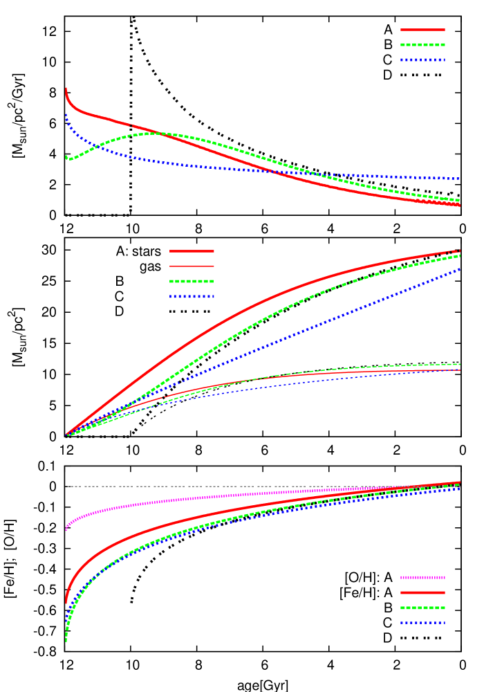
Figure 16: Upper panel: Gas infall rates for models A–D. Middle panel: Cumulative stellar and gas surface density (thick and thin lines, respectively). Lower panel: Metal enrichment laws [Fe/H] of models A–D. The horizontal thin black line at solar metallicity is for guiding the eye. Additionally the oxygen enrichment [O/H]=0.375[Fe/H] is shown for model A (pink dotted line).

4.7 Thick disc

The thick disc properties in the solar neighbourhood are not well determined. In many investigations a local stellar contribution of $\sim 5\%$ and a velocity dispersion of $\sim$45 km/s are adopted. These values lead to a dominance of thick disc stars compared to the thin disc at distances $z>1$ kpc which is directly observed for K dwarfs (Phleps et al., 2005). But in a recent paper local contributions up to 20% and metallicities up to solar are claimed (Bensby et al., 2007). Since the method of the latter paper relies on a statistical separation from the kinematics by adopting Gaussian velocity distribution functions for the thin and for the thick disc, it underestimates strongly the thin disc contribution at the high velocity tail. In our models we use standard values for the thick disc and investigate the influence of the thick disc on the other model properties. We split the local stellar density into a thin disc and a thick disc component. For models A–D we set $\sigma_{\mathrm{t}}\sim 45$ km/s and choose $\Sigma_{\mathrm{t}}$ leading to a local stellar mass contribution of $\sim 5\%$. The local mass fraction of the thick disc equals the thin disc density at $z=1.1-1.25$ kpc in the models. We adopt an age of 12 Gyr for the thick disc leading to two consequences. Firstly the high mass end of the MS is missing and the fraction in number of low mass stars is a factor of 1.84 larger than the mass fraction. This has to be taken into account when comparing to results of star counts. For model A the number of K dwarfs in the thick disc equals that in the thin disc at $z=950$ pc very close to the observed K dwarf density profile of Phleps et al. (2005). Secondly for the kinematics $f(|W|)$ the thick disc contribution is only taken into account for stars with lifetime larger than 12 Gyr. Here the correction factor 1.84 is also included.

In all cases the density profile of the thick disc can be fitted by a sech${}^{\alpha}(z/\alpha h_{\mathrm{t}})$ profile to better than 3%. The corresponding best fit coefficients are given in table 2. For the thin disc profile a corresponding fit deviates up to 25%.

We have calculated two alternative thick discs in model A with smaller and larger velocity dispersion, respectively. The surface density of the thick discs are adjusted to yield the same crossing point of the thin and thick disc profile (upper panel of figure 17). the local density contributions of the thick discs are 5.7%, 8.6% and 4.9% for discs 1,2, and 3, respectively. The contribution of the thick disc to the velocity distribution function is shown in the lower panel of Fig. 17. All these models are still consistent with the data in the $|W|$-range of 40–60 km/s. From the distribution functions we can conclude that a kinematically distinct thick disc cannot exceed a local density contribution of 10% in mass density.

Model E is a model without thick disc component but with the same AVR and SFR as in model A. For the minimum $\chi^{2}$ no alteration in the AVR and SFR are needed. The best fit $\sigma_{\mathrm{e}}$ is slightly higher. The total star formation $S_{0}$ and the densities of the thin disc are larger containing now all stars in the solar neighbourhood. The corrections to all other parameters are within a few percent. The effect of the thick disc on the velocity distribution function of stars with lifetime larger than 12 Gyr is shown in the lower panel of Fig. 17. Only the high velocity tail is affected.

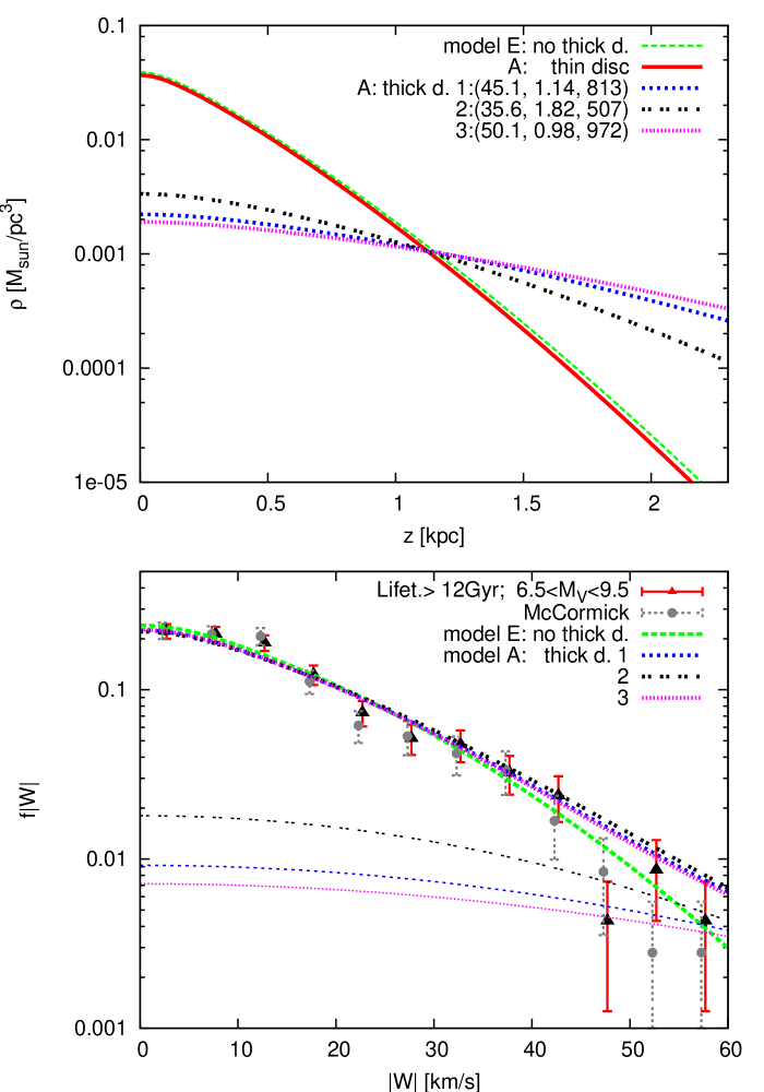
Figure 17: Upper panel: Density profiles of models with different isothermal thick disc components: Thin disc stars of model E without thick disc and model A with different thick discs; thick disc parameters ($\sigma_{\mathrm{t}},\alpha,h_{\mathrm{t}}$) are indicated. Lower panel: Reproduction of $f|W|$ from the last two plots of figure 6, but in log-scale to demonstrate the effect of the thick disc contribution. Thick lines are the combined distribution functions and thin lines are the thick discs only.

4.8 Initial mass function

We have fixed the IMF for the best fitting process (equation 27). We can use the local luminosity function to test the adopted IMF. For the determination of the IMF from the local luminosity function, the luminosity function is first converted to a mass function $dN=f(M)dM$ using the transformation formulae of Henry & Mc Carthy (1993), corrected in Henry et al. (1999), and extended to bright stars according to Schmidt-Kaler in Schmidt-Kaler (1982), which was confirmed by Andersen (1991). The star numbers are normalised to a sphere with radius R=20 pc. The result is shown in the lower panel of Fig. 18 and compared to the PDMF given in Kroupa et al. (1993) (KTG93). In our model we use the system mass function excluding resolved B components of binaries. In addition turnoff stars were excluded to be consistent with the main sequence lifetimes used in the dynamical model. Therefore our PDMF is systematically below KTG93. The PDMF is also corrected for the vertical gradient of the density profiles in the observed volume. In the brightest bin with lifetime 0.15 Gyr the density in the mid-plane is 50% larger than the mean density in the 200 pc sphere.

In order to determine the conversion factor from the local PDMF to the IMF due to the finite lifetime and the vertical thickness $h_{\mathrm{ms}}$, the main sequence lifetime is needed. We use the lifetimes estimated from the stellar evolution tracks shown in Fig. 2 for the different magnitude bins, where the metal enrichment and the relative weighting due to the increasing number of stars with decreasing mass in the mass interval is taken into account. These data are shown in the upper right panel of Fig. 18 with a comparison of the lifetimes determined directly from evolutionary tracks of Girardi et al. (2004) and with the analytic fitting formula of Eggleton et al. (1989). Any systematic variation of the lifetimes result in significant changes of the conversion factor and therefore the IMF. The conversion factors are a combination of the dilution by the increasing thickness with age (measured by $h_{\mathrm{ms}}$) and the fraction of born stars still on the main sequence due to the finite lifetime. The last factor depends strongly on the SFR. The upper left panel of Fig. 18 shows the conversion factor (=IMF/PDMF) as a function of lifetime at different heights above the mid-plane for model A.

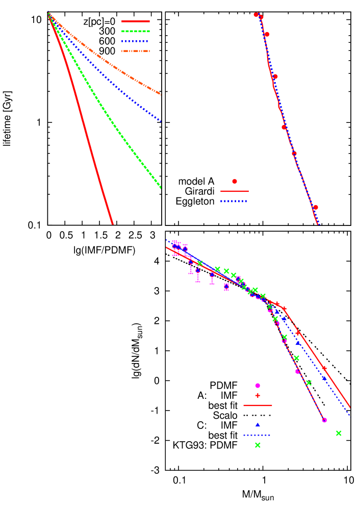
Figure 18: Upper left panel: Conversion factor (=IMF/PDMF) for model A that must be applied to the PDMF to derive the normalised IMF from local star counts. Upper right panel: Stellar lifetimes as function of stellar mass to relate the conversion factors at the left to the PDMF below. Dots are the values used in the models (from Fig. 2) and lines are values determined by Girardi et al. (2004) and Eggleton et al. (1989). Lower panel: Full circles show the PDMF of our sample and crosses the PDMF of KTG93. The IMF from models A and C are given by the plus signs and the triangles, respectively. The best fit IMF and corresponding PDMF for model A (full red lines) and model C (dotted blue lines) are over-plotted. The dashed black lines show the Scalo IMF and IMF for comparison.

In the lower panel of Fig. 18 the PDMF and the IMFs of model A and C are shown with different symbols. The IMFs of model B and D are very similar to that of model A. We compared different best fits in log-scale to test the significance of different IMFs. The highest mass bin is not consistent with the Scalo IMF (Eq. 27), but the dominating contribution to the rms value of 4.98 originates from the mass range $0.4<M/\rm{M}_{\mathrm{\rm\sun}}<1$. A similar best fit of a Kroupa IMF KTG93 (Kroupa et al., 1993) leads to a rms value of 5.67 for $\alpha=-2.7$ at $M/\rm{M}_{\mathrm{\rm\sun}}>1.0$. If we allow the slope of the Scalo IMF to vary at the high mass end for $M/\rm{M}_{\mathrm{\rm\sun}}>2.0$ we find a best fit value of $\alpha=-4.16$ and a rms of 2.81. A similar best fit of a Kroupa-like IMF as used in Aumer & Binney (2009) leads to $\alpha=-3.06$ at $M/\rm{M}_{\mathrm{\rm\sun}}>1.0$ with rms=5.96.

An inspection of the shape of the IMFs of models A and C shows that the break near 1 $\rm{M}_{\mathrm{\rm\sun}}$ seems artificial. The break is obvious in the PDMF, but the reason for this is that the correction factor due to the finite lifetime starts to apply above $\sim 1\rm{M}_{\mathrm{\rm\sun}}$. Therefore we determined an alternative IMF by fitting power laws in two mass regimes only, where we fixed the break mass $M_{0}$ by minimising the rms of the best fit. The best fits are

$$\mbox{\rm d}N/\rm{M}_{\mathrm{\rm\sun}} = N_{0}\left(M/\rm{M}_{\mathrm{\rm\sun}}\right)^{\alpha}\mbox{\rm d}\left(M/\rm{M}_{\mathrm{\rm\sun}}\right)\quad\mathrm{with}$$ (36)

$$A:\,\alpha = \left\{\begin{array}[]{rcl}-1.46\pm 0.10&&0.08\leq M/\rm{M}_{\mathrm{\rm\sun}}<1.72\\ -4.16\pm 0.12&&1.72\leq M/\rm{M}_{\mathrm{\rm\sun}}<6.0\end{array}\right.$$

$$N_{0}=272/\rm{M}_{\mathrm{\rm\sun}}\quad\mathrm{at}\quad M_{0}/\rm{M}_{\mathrm{\rm\sun}}=1.72\,,$$

$$C:\,\alpha = \left\{\begin{array}[]{rcl}-1.70\pm 0.13&&0.08\leq M/\rm{M}_{\mathrm{\rm\sun}}<1.35\\ -4.07\pm 0.11&&1.35\leq M/\rm{M}_{\mathrm{\rm\sun}}<6.0\end{array}\right.$$

$$N_{0}=388/\rm{M}_{\mathrm{\rm\sun}}\quad\mathrm{at}\quad M_{0}/\rm{M}_{\mathrm{\rm\sun}}=1.35\,,$$

where $N_{0}$ gives the normalisation in the 20 pc sphere. The slopes at the high mass end are very similar for models A–D, because the IMFs are essentially shifted vertically relative to each other. The best fits of the Kroupa-like IMFs show that forcing the slope in the mass range $1-1.5\rm{M}_{\mathrm{\rm\sun}}$ to be the same as at the high mass end results in a flatter IMF and a much larger rms value. At that stage of the investigation we abstain from final conclusions, because we did not discuss possible biases in the PDMF from local star counts. We expect that the feedback of a corrected IMF with a steeper slope at the high mass end to the disc model via the mass loss is very small. Additionally it affects only the velocity distribution functions for lifetimes smaller than $10^{8}$ yr significantly.

The strongest constraints on the IMF at high masses and the present day SFR is the observed number of A and late B stars in the solar neighbourhood. Since the bright stars with $M_{\mathrm{V}}<0.5$ mag are observed in a sphere with a radius of 200 pc, the sample size is a direct measure of the local surface density. Therefore the conversion from the IMF to the mean SFR in the last few 100 Myr depends only on the lifetime of the stars. That means, a higher present day SFR requires a shorter lifetime for the A stars or a steeper IMF.

As an example the constant SFR used in the Besançon model (Robin et al., 2003) relies mainly on the assumption of a steep IMF in the stellar mass range 1-3 $\rm{M}_{\mathrm{\rm\sun}}$ (Haywood et al., 1997b). This model and also the SFR determination of Vergely et al. (2002) show that the slope of the IMF in the mass range of 1-3 $\rm{M}_{\mathrm{\rm\sun}}$ that covers roughly the lifetime range of 0.2-10 Gyr, is crucial for the derivation of the long-term SFR from star counts. A steep IMF in that mass range introduces a strong bias to young ages, because the observed number of stars above 2 $\rm{M}_{\mathrm{\rm\sun}}$ predict too many young lower mass stars via the steep IMF. This effect is strengthened by the fitting procedure, because direct age determinations by isochrone fitting are less significant in the lower mass range. The result is a bias to young ages in the stellar mass range covering the lifetime above 1 Gyr. An underestimation of the SFR for ages above 1 Gyr is the consequence.

The position of the Sun is probably about 20 pc above the mid-plane (Humphreys & Larsen, 1995). For the determination of the mid-plane density this offset can play a significant role for sub-populations with small scale height ($M_{\mathrm{V}}<1.5$ mag). We corrected for that implicitly, since we determined the mid-plane density of these magnitude bins for the PDMF using spheres with large radii (see Table 1), where the offset can be neglected.

5 Summary

We presented a new disc model for the thin disc in the solar cylinder based on a continuous star formation history (SFR) and a continuous dynamical heating law (AVR) of the stellar sub-populations. This new model combines and improves the advantages of several different attempts to model the vertical structure in the solar neighbourhood: We used a sequence of isothermal sub-populations in dynamical equilibrium as Bahcall & Soneira (1984) and Aumer & Binney (2009) did; We used the full velocity distribution functions $f|W|$ as Holmberg & Flynn (2000) did, and not only the velocity dispersions (the AVR); We solved the Poisson equation self-consistently including the thick disc, gas and DM halo contribution as done in the Besançon model (Robin et al., 2003). A chemical evolution model with reasonable gas infall rate, which was tuned to reproduce the local [Fe/H] distribution of G dwarfs, is included. This enables us to apply correct MS luminosities and lifetimes. Additionally our model is insensitive to the IMF, because it is based on the normalised velocity distribution functions of MS stars.

We determined pairs of (SFR, AVR) by a best fit of the local kinematics. The SFRs which are consistent with the MS velocity distribution functions show a decline factor below five down to unity (= const. SFR). The strongest feature that would distinguish between a constant and a declining SFR is a direct determination of the age distribution of low mass stars in the solar neighbourhood.

Despite the large variety of SFRs there is a strong correlation to the AVR. For each SFR the slope and maximum velocity dispersion of the AVR are well determined. For the AVR we find a power law with indices between 0.375 and 0.5. The range of models is consistent with the results of Binney et al. (2000) for the local age distribution and Aumer & Binney (2009) for the SFR.

Applying the stellar lifetimes and the new scale height corrections to the PDMF results in an IMF that shows only one break point at $1.7\rm{M}_{\mathrm{\rm\sun}}$ and a steep falloff at high masses.

The density profile of an isothermal thick disc component can be fitted very good by a sech${}^{\alpha}_{\mathrm{t}}$ profile, where $\alpha_{\mathrm{t}}$ depends on the velocity dispersion. The most prominent effect of thick disc stars is the enhancement of the high velocity wings of K and M dwarfs in the range of 40–60 km/s. From that we can exclude a heavy thick disc with distinct kinematics and more than 10% contribution to the local stellar density. Changing the thick disc parameters leads to slight variations of the thin disc properties (mainly by assigning part of the stellar disc to the thick disc), but has a negligible influence on the normalised SFR and AVR of the thin disc.

A variety of predictions can be made from the new disc model. The density profiles of MS star sub-populations depend on the lifetime of the stars and are significantly different to density profiles of single age sub-populations. The shape is neither exponential nor sech² and can be characterised by the (half-)thickness and the exponential scale height. From the vertical density profiles MS stars number densities as function of colour and apparent magnitude can be predicted. Applying these number densities with observed ’Hess’ diagrams from large surveys like the catalogues of the Sloan Digital Sky Survey SEGUE/SDSS enables us to restrict the parameters of the SFR further. We determined vertical gradients in the kinematics which will be tested with Radial Velocity Experiment (RAVE) data. Age and metallicity distributions of stellar sub-populations as a function of $z$ above the galactic plane are predicted.

The future plan is to extend the local model to a complete disc model of the Milky Way that provides a fully self-consistent connection of stellar densities and kinematics. Ultimately this kind of detailed model is essential to understand the large data sets as already available from SDSS and which are expected on a much higher level in amount and precision by PanSTARRS and the astrometric Gaia satellite mission.

References

- Abazajian et al. (2009) Abazajian, K. N., Adelman-McCarthy, J. K., Agüeros, M. A. K., et al. 2009, ApJS, 182, 543
- Andersen (1991) Andersen, J., 1991, A&ARev. 3, 91
- Aumer & Binney (2009) Aumer M., Binney J.J. 2009, MNRAS, 397, 1286
- Bahcall (1984a) Bahcall, J. N. 1984a, ApJ, 276, 156
- Bahcall (1984b) Bahcall, J. N. 1984b, ApJ, 276, 169
- Bahcall & Soneira (1980a) Bahcall, J. N., Soneira, R. M. 1980, ApJS, 44, 73
- Bahcall & Soneira (1980b) Bahcall, J. N., Soneira, R. M. 1980, ApJ, 238, L17
- Bahcall & Soneira (1984) Bahcall, J. N., Soneira, R. M. 1984, ApJS, 55, 67
- Bailer-Jones (2005) Bailer-Jones, C. A. L., 2005, in ’Transits of Venus: New Views of the Solar System and Galaxy’, Proc. of IAU Coll. 196, ed. D.W. Kurtz, Cambridge University Press, 429
- Bensby et al. (2007) Bensby, T., Zenn, A. R., Oey, M. S., Feltzing, S. 2007, ApJ 663, L13
- Bertelli et al. (1994) Bertelli, G., Bressan, A., Chiosi, C. et al. 1994, A&AS, 106, 275
- Binney et al. (2000) Binney, J., Dehnen, W., Bertelli, G. 2000, MNRAS 318, 658
- Bronfman et al. (1988) Bronfman L., Cohen R. S., Alvarez H., May J., Thaddeus P. 1988, ApJ 324, 248
- Cignoni et al. (2006) Cignoni M., Degl’Innocenti S., Prada Moroni P. G., Shore S. N. 2006, A&A 459, 783
- Dehnen & Binney (1998) Dehnen, W., Binney, J. 1998, MNRAS 298, 387
- Delhaye (1965) Delhaye, J. 1965, in Galactic Structure, Stars and Stellar Systems 5, 61
- R. & C. de la Fuente Marcos (2004) de la Fuente Marcos R., de la Fuente Marcos C. 2004, NewA 9, 475
- Dickey & Lockman (1990) Dickey J. M., Lockman F. J. 1990, ARAA 28, 215
- Eggleton et al. (1989) Eggleton P. P., Fitchett M. J., Tout C. A. 1989, ApJ, 347, 998
- Fioc & Rocca-Volmerange (1997) Fioc M., Rocca-Volmerange B. 1997, A&A 326, 950
- Freeman (1991) Freeman, K. C. 1991, in Sundelius B., Dynamics of Disc Galaxies. Göteborg Observatory, Göteborg, 15
- Girardi et al. (2002) Girardi L., Bertelli G., Bressan A., Chiosi C., Groenewegen M.A.T., Marigo P., Salasnich B., Weiss A. 2002, A&A 391, 195
- Girardi et al. (2004) Girardi L., Grebel E. K., Odenkirchen M., Chiosi C. 2004, A&A 422, 205
- Haywood et al. (1997a) Haywood M., Robin A. C., Créze M. 1997a, A&A 320, 428
- Haywood et al. (1997b) Haywood M., Robin A. C., Créze M. 1997b, A&A 320, 440
- Haywood (2006) Haywood M. 2006, MNRAS 371, 1760
- Henry & Mc Carthy (1993) Henry T. J., Mc Carthy D. W. Jr. 1993, AJ 106, 773
- Henry et al. (1999) Henry T. J., Franz O. G., Wasserman L. H. L. et al. 1999, ApJ 512, 864
- Hernandez et al. (2000) Hernandez X., Valls-Gabaud D., Gilmore G. 2000, MNRAS, 316, 605
- Holmberg & Flynn (2000) Holmberg J., Flynn C. 2000, MNRAS, 313, 209
- Holmberg & Flynn (2004) Holmberg J., Flynn C. 2004, MNRAS, 352, 440
- Holmberg et al. (2009) Holmberg J., Nordström B., Andersen J., 2009, A&A, in press, arXiv:0811.3982 GCS2
- Humphreys & Larsen (1995) Humphreys R. M., Larsen J. A. 1995, AJ 110, 2183
- Jahreiß & Wielen (1997) Jahreiß H., Wielen R. 1997, In B. Battrick, M. A. C. Perryman, eds., Proc. ESA SP-402 (Nordwijk, ESA), 675
- Just & Jahreiß (2009) Just A., Jahreiß H. 2009, in preparation (Paper II)
- Just et al. (1996) Just A., Fuchs B., Wielen R. 1996, A&A 309, 715
- Just et al. (2006) Just A., Moellenhoff C., Borch A. 2006, A&A 459, 703
- Kroupa et al. (1993) Kroupa P., Tout C. A., Gilmore G. 1993, MNRAS 262, 545
- Kuijken & Gilmore (1991) Kuijken K., Gilmore G. 1991, ApJ 367, L9
- Lucy (2000) Lucy L.B.2000, MNRAS 318, 92
- Nordström et al. (2004) Nordström B., Mayor M., Andersen J., et al. 2004, A&A 418, 989, GCS1
- Perryman et al. (2001) Perryman, M. A. C., de Boer, K. S., Gilmore, G., Høg, E., Lattanzi, M. G., Lindegren, L., Luri, X., Mignard, F., Pace, O., de Zeeuw, P. T., 2001, A&A 369, 339
- Phleps et al. (2005) Phleps S., Drepper S., Meisenheimer K., Fuchs B. 2005, A&A 443, 929
- Pont & Eyer (2005) Pont F., Eyer L. 2005 in Proc. Gaia Symposium ’The Three-Dimensional Universe with Gaia’ (ESA SP-576), Eds. C. Turon, K.S. O’Flaherty, M.A.C. Perryman, 187
- Press et al. (1992) Press W. H., Teukolsky S. A., Vetterling W. T., Flannery B. P. (eds.), Numerical Recipes, Cambridge University Press, 1992
- Reddy et al. (1993) Reddy B. E., Tomkin, J., Lambert D. L., Allende Prieto C. 2003, MNRAS 340, 304
- Rocca-Pinto et al. (2000) Rocca-Pinto H. J., Scalo J., Maciel W. J., Flynn C. 2000, A&A 358, 869
- Robin et al. (2003) Robin A. C., Reylé C., Derrière S., Picaud S. 2003, A&A 409, 523
- Roskar et al. (2008) Roskar R., Debattista V. P., Quinn T. R., Stinson G. S., Wadsley J. 2008, ApJ 684, L79
- Scalo (1986) Scalo J. M. 1986, Fundamentals of Cosmic Physics 11, 1
- Schmidt-Kaler (1982) Schmidt-Kaler T. 1982, in Landolt-Börnstein Vol. 2, 4.1
- Schönrich & Binney (2009) Schönrich R., Binney J. 2009, MNRAS 396, 203
- Sellwood & Binney (2002) Sellwood J. A., Binney J. 2002, MNRAS 336, 785
- van Leeuwen (2007) van Leeuwen F. 2007, Hipparcos, the new Reduction of the Raw Data, Springer Dortrecht
- Vergely et al. (2002) Vergely, J.-L., Köppen, J., Egret, D., Bienaymé, O. 2002, A&A 390, 917
- Vyssotsky (1963) Vyssotsky A. N. 1963, in Basic Astronomical Data, Stars and Stellar Systems 3, 192
- Wilson & Woolley (1970) Wilson O., Woolley R. 1970, MNRAS 148, 463
- Wielen (1977) Wielen R. 1977, A&A 60, 263
- Wielen et al. (1996) Wielen R., Fuchs B., Dettbarn C. 1996, A&A 314, 438
- Zwitter et al. (2008) Zwitter, T., Siebert, A., Munari, U., et al. 2008, AJ 136, 421