New universal conductance fluctuation of mesoscopic systems in the crossover regime from metal to insulator

Abstract

We report a theoretical investigation on conductance fluctuation of mesoscopic systems. Extensive numerical simulations on quasi-one dimensional, two dimensional, and quantum dot systems with different symmetries (COE, CUE, and CSE) indicate that the conductance fluctuation can reach a new universal value in the crossover regime for systems with CUE and CSE symmetries. The conductance fluctuation and higher order moments vs average conductance were found to be universal functions from diffusive to localized regimes that depend only on the dimensionality and symmetry. The numerical solution of DMPK equation agrees with our result in quasi-one dimension. Our numerical results in two dimensions suggest that this new universal conductance fluctuation is related to the metal-insulator transition.

One of the most important features in mesoscopic system is that the conductance in the diffusive regime exhibits universal features with a universal conductance fluctuation (UCF) that depends only on the dimensionality and the symmetry of the system.lee85 There exist three ensembles or symmetries according to the random matrix theory (RMT)beenakker : (1). Circular orthogonal ensemble (COE) (characterized by symmetry index $\beta=1$) when the time-reversal and spin-rotation symmetries are present. (2). Circular unitary ensemble (CUE) ($\beta=2$) if time-reversal symmetry is broken. (3). Circular symplectic ensemble (CSE) ($\beta=4$) if the spin-rotation symmetry is broken while time-reversal symmetry is maintained. In the diffusive regime, the UCF is given by $rms(G)=c_{d}/\sqrt{\beta}e^{2}/h$ where $c_{d}=0.73,0.86,0.70$ for quasi-one dimension (1D), two dimensions (2D) and quantum dot (QD) systems and $\beta=1,2,4$.lee85 ; beenakker Although the RMT can apply to both diffusive and localized regimes, so far the universal conductance fluctuation has been addressed and established only in the diffusive regime. When the system is away from the diffusive regime, some universal behaviors have been observed. For instance, the conductance distribution of quasi-1D systems ($\beta=1$) with surface roughness was found to be universal in the crossover regime, independent of details of the system.saenz1 For quasi-1D systems with $\beta=1,2$ the conductance distribution obtained from tight-binding model agrees with the numerical solution of DMPK equation.saenz2 In the localized regime, the conductance distribution of the quasi-1D system obeys log normal distribution.wolfle In high dimensions, conductance distribution at the mobility edge of metal-insulator transition was also shown numerically to be universal for 2D systems with $\beta=2,4$ and a 3D system with $\beta=1$.soukoulis In the localized regime, the conductance distribution of 3D systems is qualitatively different from that of quasi-1D systems.wolfle1 It would be interesting to further explore the universal behaviors of these systems and ask following questions: Is there any universal behaviors away from mobility edge? Is it possible to have a UCF beyond the diffusive regime? If there is, what is the nature of the new UCF? It is the purpose of this work to investigate these issues.

To do this, we have carried out extensive numerical calculations for conductance fluctuations $rms(G)$ in quasi-1D, 2D and QD systems for different symmetries: $\beta=1,2,4$. Our results can be summarized as follows. (1). From diffusive to localized regimes, the conductance fluctuation and higher order moments were found to be universal functions of the average conductance for quasi-1D, 2D, and QD systems and for $\beta=1,2,4$. (2). We found that there exists a second UCF near the localized regime for $\beta=2,4$ but not for $\beta=1$. Our results show that the new UCF depends weakly on the symmetries of the system and assumes the following value: $rms(G)={\tilde{c}}_{d}e^{2}/h$. Here for $\beta=2$ we found ${\tilde{c}}_{d}=0.56\pm 0.01,0.68\pm 0.01,0.58\pm 0.01$ for quasi-1D, 2D and QD systems, respectively while for $\beta=4$ we have ${\tilde{c}}_{d}=0.55\pm 0.01,0.66\pm 0.02,0.56\pm 0.01$. The conductance distribution in this new regime was found to be one-sided log-normal in agreement with previous results.wolfle (3). In the localized regime with $\left\langle G\right\rangle<0.3$, the conductance distribution does not seem to depend on dimensionality and symmetry. (4). For quasi-1D systems, the numerical solution of DMPK equationdmpk agrees with our results. (5). For quasi-1D systems, the new UCF occurs when the localization length $\xi$ is approximately equal to the system size $L$, i.e., $\xi\sim L$ for $\beta=2,4$. For 2D systems, we found that the new UCF occurs in the vicinity of the critical region of metal-insulator transition.

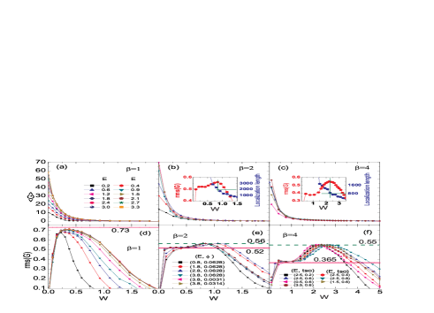
Figure 1: (Color online) Average conductance (a,b,c) and its fluctuation (d,e,f) vs disorder strength $W$ for different symmetry index $\beta$ in quasi-1D systems. Insets: localization length vs $W$ for $\beta=2,4$.

In the numerical calculations, we used the same tight-binding Hamiltonian as that of Ref.qiao, . Static Anderson-type disorder is added to the on-site energy with a uniform distribution in the interval $[-W/2,W/2]$ where $W$ characterizes the strength of the disorder. The conductance $G$ is calculated from the Landauer-Buttiker formula $G=({2e^{2}}/{h})T$ with $T$ the transmission coefficient. The conductance fluctuation is defined as $\text{rms}(G)\equiv\sqrt{\left\langle G^{2}\right\rangle-\left\langle G\right\rangle^{2}}$, where $\left\langle{\cdots}\right\rangle$ denotes averaging over an ensemble of samples with different disorder configurations of the same strength $W$. In the following the average conductance and its fluctuation are measured in unit of $e^{2}/h$; the magnetic field is measured using magnetic flux $\phi=\mu_{B}B/t$ where $\mu_{B}$ is Bohr magneton and $t$ is the hopping energy that is used as the unit of energy.

We first examine average conductances $\left\langle G\right\rangle$ and their fluctuations $rms(G)$ vs disorder strength $W$ in quasi-1D systems with different symmetry index $\beta$ (see Fig.1). In our numerical simulation, the size of quasi-1D systems are chosen to be $40\times 2000$ for $\beta=1,2$ (Fig.1a,b) and $40\times 800$ for $\beta=4$ (Fig.1c). Each point in Fig.1 is obtained by averaging 9000 configurations for $\beta=1$ and 15000 configurations for $\beta=2,4$. In Fig.1, data with different parameters are shown. For instance with $\beta=2$, $\left\langle G\right\rangle$ and $rms(G)$ vs $W$ are plotted for different Fermi energies with fixed $\phi=0.0628$ and different magnetic flux with fixed Fermi energy $E=3.8$. From Fig.1, we see that in the diffusive regime where $\left\langle G\right\rangle>1$ there is a plateau region for $rms(G)$ with the plateau value approximately equal to the known UCF values $rms(G)=0.73/\sqrt{\beta}=0.73,0.52,0.365$ (marked by solid lines). This suggests that one way to identify UCF is to locate the plateau region in the plot of $rms(G)$ vs disorder strength and the plateau value should correspond to UCF. This method has been used to identify universal spin-Hall conductance fluctuationren that was later confirmed by RMT.confirm Importantly, there exists a second plateau region for $\beta=2,4$ but not for $\beta=1$. The new plateau value approximately equals to $rms(G)=0.56\pm 0.01$ for $\beta=2$ and $rms(G)=0.55\pm 0.01$ for $\beta=4$. In this regime, we found that $\left\langle G\right\rangle\leq 1$ which clearly corresponds to the crossover regime. To confirm that the first and second plateaus are indeed in the diffusive and crossover regimes, respectively, we have calculated the localization length $\xi$ of the quasi-1D system (insets of Fig.1). It is clear that near the first plateau where $W\sim 0.4$ for $\beta=2$ and $W\sim 1$ for $\beta=4$ we have $\xi\gg L$ with $L$ the length of quasi-1D system while near the second plateau we have $\xi\sim L$ (see insets of Fig.1).

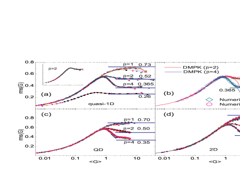
Figure 2: (Color online) Conductance fluctuation vs average conductance for quasi-1D systems (a,b), QD systems (c), and 2D systems (d).

According to the UCF in the diffusive regime, it is tempting to conclude that this second plateau should correspond to a new UCF. However, in making such a claim one has to answer following questions: (1). whether the plateau behavior is universal? (2). if it is, whether it can be observed in a wide range of parameters? (3). how is our result compared with the theoretical predictions whenever available? (4). whether such a universal behavior exists in high dimensions? In the following, we provide evidences that the new plateau indeed corresponds to a new UCF.

To answer the first question, we plot $rms(G)$ vs $\left\langle G\right\rangle$ in Fig.2a by eliminating $W$. The fact that all curves shown in Fig.1 with different parameters (Fermi energy $E$, magnetic flux $\phi$, and SOI strength $t_{so}$) collapse into a single curve for each $\beta$ strongly indicates that $rms(G)$ vs $\left\langle G\right\rangle$ is universal. To further demonstrate this universal behavior, we have calculated the conductance fluctuation for a quasi-1D system with both magnetic flux and Rashba SOI. Although the Hamiltonian of this system is still unitary, both time reversal and spin rotation symmetries are broken. According to the diagrammatic perturbation theoryfeng , the UCF is reduced by a factor of 2 when SOI is turned on. From RMT point of view, both systems ($B\neq 0$, $t_{so}=0$) and ($B\neq 0$, $t_{so}\neq 0$) are unitary ensembles and obey the same statistics. The fact that energy spectrum for ($B\neq 0$, $t_{so}=0$) is doubly degenerate accounts for the factor of 2 reduction for the system ($B\neq 0$, $t_{so}\neq 0$). In Fig.2a, we have plotted $rms(G)$ vs $\left\langle G\right\rangle$ for the system with ($B\neq 0$, $t_{so}\neq 0$). Once again, we see that all data from different parameters collapse into a single curve. If we multiply this curve by a factor of 2, it collapses with the curve of $\beta=2$ (see inset of Fig.2a).

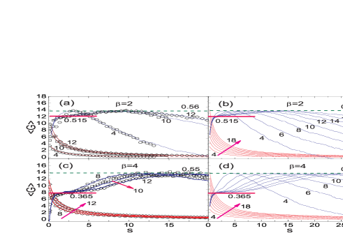
Figure 3: (Color online) Average conductance and its fluctuation vs s for quasi-1D systems [(a) and (c)] and compared with results of DMPK equation for different $N=4,6,...,18$ [(b) and (d)]. The arrow points the direction of increasing $N$.

From Fig.2a we see that in the diffusive regime with $\left\langle G\right\rangle>1$ the long plateau for each $\beta$ corresponds to the known UCF (marked by solid lines). For $\beta=1$ there is only one plateau. For $\beta=2,4$, however, a second plateau region is in the neighborhood of $\left\langle G\right\rangle\sim 1$. For $\beta=2$, $rms(G)$ is approximately a constant hence universal in the region $\left\langle G\right\rangle=(0.6,1.4)$ while for $\beta=4$ this region narrower with $\left\langle G\right\rangle=(0.7,0.9)$. Looking at Fig.2a, it seems that the second plateau region is narrower than the first one. But if we look at $rms(G)$ vs $W$ where $W$ can be controlled experimentally, the crossover region is enlarged since in the crossover regime $\left\langle G\right\rangle$ is not very sensitive to $W$ while in the diffusive regime it is the opposite. Indeed, in Fig.1f, we do see that the ranges of the first and second plateau regions are comparable. If we fix $W$ and plot $\left\langle G\right\rangle$ and $rms(G)$ vs the length of the system, the crossover regime is enlarged further. These results are shown in Fig.3a,c where the symbols represent our numerical result and solid lines correspond to exact solution of DMPK equation (to be discussed below). We see that the window of the second plateau is much larger than the first one.

Since the statistics of transmission eigen-channels of quasi-1D systems can be described by DMPK equation, we have numerically solved itshi for $\beta=2,4$ and compared our numerical results of tight-binding model with that of DMPK. Fig.3b and Fig.3d show the numerical solution of DMPK equation for $\beta=2,4$ with different $N=4,6,...,18$ where $N$ is the number of transmission channels. Here $s=L/{\bar{l}}$ where $L$ is the length of quasi-1D systems and ${\bar{l}}$ is the average mean free path.beenakker ; new Fig.3 clearly shows that in the diffusive regime where $1\ll s\ll N$ the first plateau corresponds to the usual UCF and there exists a much wider second plateau in the crossover regime where $s$ and $N$ are comparable with plateau value equal to our newly identified UCF. Fig.3a and Fig.3c show the comparison between the results of DMPK and that of quasi-1D tight binding model. The $rms(G)$ vs $\left\langle G\right\rangle$ of DMPK equation is plotted in Fig.2b where selected data from Fig.2a is also plotted for comparison. The agreement between numerical and theoretical results is clearly seen.

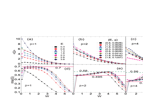
Figure 4: (Color online) Average conductance and its fluctuation vs $W$ for QD systems with $\beta=1,2,4$.

Now we examine the conductance fluctuation for QD systems. In the numerical calculation, the size of QD is $L\times L$ with $L=100$ and the width of the lead $L_{0}=10$ for $\beta=2,4$ while for $\beta=1$ we used $L=150$. Fig.4 depicts $\left\langle G\right\rangle$ and $rms(G)$ vs $W$ for $\beta=1,2,4$. Each point in Fig.4 was obtained by averaging 9000 configurations for $\beta=1$ and 20000 configurations for $\beta=2,4$. Similar to quasi-1D systems, we see only one plateau region in the diffusive regime for $\beta=1$ with plateau value close to the known UCF value $rms(G)=0.70$. In addition to the first plateau in the diffusive regime, there exists a second plateau for $\beta=2,4$ which we identify to be the regime for new UCF. The new UCF is again in the crossover regime where $\left\langle G\right\rangle\sim 1$ with the value ${\rm UCF}(\beta=2)=0.58\pm 0.01$ and ${\rm UCF}(\beta=4)=0.56\pm 0.01$. In Fig.2c we plot $rms(G)$ vs $\left\langle G\right\rangle$. It shows that all curves for each $\beta$ collapse into a single curve showing universal behaviors. Fig.4e and Fig.4f show that the new universal regime can be quite large. Finally we have also calculated the conductance fluctuation for 2D systems and similar behaviors were found (see Fig.2d).foot4 In particular, the values of new UCF are found to be ${\rm UCF}(\beta=2)=0.68\pm 0.02$ and ${\rm UCF}(\beta=4)=0.66\pm 0.01$.

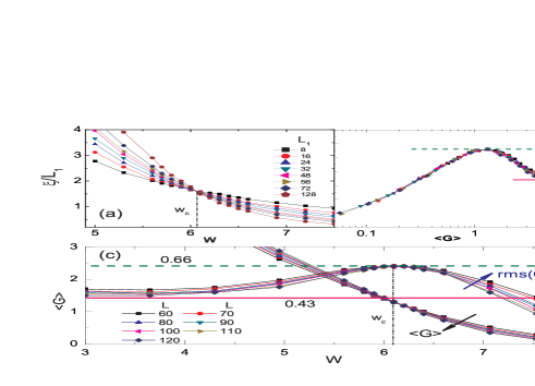
Figure 5: (Color online) Localization length, average conductance, conductance fluctuation of 2D symplectic systems for different $L$ with $E=2.3$ and $t_{so}=0.4$. (a). $\xi/L_{1}$ vs $W$. (b). $rms(G)$ vs $\left\langle G\right\rangle$ for different $L=60,70,...,120$. (c). $rms(G)$ and $\left\langle G\right\rangle$ vs $W$.

Now we provide further evidence of the universal behavior of new UCF. In 2D systems there can be a metal-insulator transition (MIT) for $\beta=2,4$ but not for $\beta=1$. This somehow coincides with our findings that there is a new UCF regime for $\beta=2,4$ but not for $\beta=1$. To explore this correspondence further, we have calculated the localization length of the 2D system using the transfer matrix approach.mac Here we calculate the localization length $\xi$ for quasi-1D systems with fixed length $1000000$ and different widths $L_{1}$ (see Fig.5a). Fig.5a depicts the localization length $\xi/L_{1}$ vs disorder strength for $\beta=4$. The intersection of different curves gives an estimate of the critical disorder strength of MIT of the 2D system. Fig.5a shows that for an infinite 2D system, there is a MIT around $W_{c}=6.1$. For a mesoscopic 2D system, the critical region becomes a crossover region around the same $W_{c}$ and it is in this region where the new UCF is found. To see how our new UCF evolves with increasing of system size $L$ we have calculated $rms(G)$ vs $W$ for finite 2D systems with different sizes $L=50+10n$ where $n=1,2,...,7$. As shown in Fig.5c, for a fixed $W$ that is beyond the crossover regime, e.g., $W=7$, the fluctuation decreases as $L$ increases so that $rms(G)\rightarrow 0$ at $L\rightarrow\infty$. Importantly, the second plateau value (the new UCF) does not change with $L$. In addition, both $\left\langle G\right\rangle$ and $rms(G)$ converge at $W_{c}=6.1$ for different $L$. This means that when $L$ goes to infinity we should have $rms(G)=c_{\beta}$ in the vicinity of critical region where $c_{\beta}$ is the new UCF. This again suggests that the new UCF is driven by MIT and is an universal quantity. Finally $rms(G)$ vs $\left\langle G\right\rangle$ is plotted in Fig.5b for different $L$ which shows the universal behavior that is also independent of $L$. Similar behaviors were also observed for 2D systems with $\beta=2$.

We have further calculated the third and fourth moments ($\gamma_{1}$ and $\gamma_{2}$) of conductance vs the average conductance.ren2 For QD and 2D systems similar universal features found in $rms(G)$ were also found for $\gamma_{1}$ and $\gamma_{2}$ with different $\beta$.attach1 It is interesting that in the localized regime with $\left\langle G\right\rangle<0.3$ the conductance distribution seems to be superuniversal that is independent of dimensionality and symmetry.attach2

In summary, we have carried out extensive simulations on conductance fluctuations of quasi-1D, QD, and 2D mesoscopic systems for orthogonal, unitary, and symplectic ensembles. Our results show that in addition to the usual UCF in the diffusive regime there exists a new UCF in the crossover regime between metallic and insulating regimes for unitary and symplectic ensembles but not for the orthogonal ensemble. We found that the conductance fluctuation $rms(G)$ and higher order moments vs $\left\langle G\right\rangle$ are universal functions from diffusive to localized regimes which depend only on symmetry index $\beta$ for quasi-1D, QD, and 2D mesoscopic systems. In quasi-1D systems this universal function agrees with the result from DMPK equation. Our analysis suggests that this new UCF is driven by MIT in 2D systems.

Acknowledgments This work was financially supported by a RGC grant (HKU 704607P) from the government of HKSAR and LuXin Energy Group. We wish to thank Prof. J.R. Shi for providing the code of solving DMPK equation. Computer Centre of The University of Hong Kong is gratefully acknowledged for the High-Performance Computing assistance.

^∗ Electronic address: jianwang@hkusua.hku.hk

References

- (1) L. B. Altshuler, JETP Lett. 41, 648 (1985); P.A. Lee and A.D. Stone, Phys. Rev. Lett. 55, 1622 (1985); P. A. Lee et al, 1987 Phys. Rev. B 35, 1039 (1987).
- (2) C.W.J. Beenakker, Rev. Mod. Phys. 69, 731 (1997).
- (3) A. Garcia-Martin and J.J. Saenz, Phys. Rev. Lett. 87, 116603 (2001).
- (4) L.S. Froufe-Perez et al, Phys. Rev. Lett. 89, 246403 (2002).
- (5) K.A. Muttalib and P. Wolfle, Phys. Rev. Lett. 83, 3013 (1999).
- (6) M. Ruhlander et al, Phys. Rev. B 64, 212202 (2001).
- (7) K.A. Muttalib et al, Phys. Rev. B 72, 125317 (2005).
- (8) O.N. Dorokhov, JETP Lett. 36, 318 (1982); P.A. Mello, P. Pereyra, and N. Kumar, Ann. Phys. (N.Y.) 181, 290 (1988).
- (9) Z.H. Qiao et al, Phys. Rev. Lett. 98, 196402 (2007).
- (10) W. Ren et al, Phys. Rev. Lett. 97, 066603 (2006).
- (11) J.H. Bardarson et al, Phys. Rev. Lett. 98, 196601 (2007).
- (12) S.C. Feng, Phys. Rev. B 39, 8722 (1989).
- (13) D.F. Li and J.R. Shi, Phys. Rev. B 79, 241303, (2009)
- (14) J. Heinrichs, Phys. Rev. B 76, 033305 (2007).
- (15) For 2d systems (in Fig.2d), we have shown data obtained from at least five different set of parameters for each .
- (16) A. MacKinnon and B. Kramer, Phys. Rev. Lett. 47, 1546 (1981); Z. Phys. B - Condensed Matter 53, 1 (1983).
- (17) W. Ren et al, Phys. Rev. B 72, 195407 (2005).
- (18) In fig.1 of EPAPS, the , and vs are plotted for QD systems (a,b,c) and 2D systems (d,e,f) with .
- (19) In fig.2 of EPAPS, the vs is depicted in fig.2a. The conductance distribution for shows universal behavior independent of dimensionality and symmetry (fig.2b) while for deviation from universal behavior is clearly seen (fig.2c).