Purity and Gaussianity bounded uncertainty relation

Abstract

Bounded uncertainty relations provide the minimum value of the uncertainty assuming some additional information on the state. We derive analytically an uncertainty relation bounded by a pair of constraints, those of purity and Gaussianity. In a limiting case this uncertainty relation reproduces the purity-bounded derived by Man’ko and Dodonov and the Gaussianity-bounded one [Phys. Rev. A 86, 030102R (2012)].

I Introduction

The only states that saturate the Schrödinger-Robertson Robertson uncertainty relation for the canonically conjugated coordinates of position and momenta, are the pure Gaussian states. However, if some additional information about the state is available then the set of states which minimize the uncertainty, or else of minimizing states (MSs), is modified while a tighter lower bound on the uncertainty can be derived.

A basic characteristic of a state is its degree of mixedeness.  The minimizing set obtained by imposing the constraint of fixed degree of mixedeness depends on the measure that one chooses to quantify this degree, i.e. purity, purities of higher order or various entropies (see Dodonov for a review).  For instance, in the case of the purity -bounded uncertainty relation suggested by Dodonov and Man’ko Man'ko the minimizing set is composed by mixed states, or more precise, mixtures of number states. On the other hand, in the case of the von-Neumann entropy, the set of the MSs is composed by the ‘thermal states’ whose temperature is increasing as the fixed entropy tends to infinity Bastiaans . In both cases, the lower bound on the uncertainty is increasing with the degree of mixedeness since the mixedeness adds extra ‘amount’ of classical (statistical) uncertainty.

In a recent work PRAr we have suggested an uncertainty relation bounded by the degree of Gaussianity, a quantity which we introduced in that same work. There the non-Gaussian MSs are identified for a fixed degree of Gaussianity and among them  one finds all the eigenstates of the harmonic oscillator. Along with the Gaussianity- bounded uncertainty relation, we have presented a general method for deriving bounded uncertainty relations that reduces the problem to an eigenvalue problem.

In this work we employ the method exhibited in PRAr to derive an uncertainty relation where the bound depends on two characteristics of the state, namely its purity and Gaussianity. To our knowledge this is the first two-dimensional bounded uncertainty relation that has been derived so far. The uncertainty relation is represented via parametric relations  which connect three quantities, namely, the purity, Gaussianity and uncertainty. This exact expression is difficult to handle analytically and for this reason we also provide an approximate expression. The derived relation provides the boundaries for three basic characteristics of a state and can be used as a tool for visualizing and partitioning the space of non-Gaussian mixed states.

The structure of the paper is the following. In first step, in Sec. II we derive the set of MSs of the purity and Gaussianity bounded uncertainty relation and then in Sec. III we provide exact and approximate expressions for this uncertainty relation. We discuss our and conclude in Sec. IV.

II Minimizing states

Let us start with the position $\hat{x}$ and momentum $\hat{p}$ of a quantum particle in one dimension, which could also be the quadratures of a single mode of the electromagnetic field, in a state defined by the density operator $\hat{\rho}$. In its most general form, the Scrödinger-Robertson  (SR) uncertainty relation Robertson for the position and momentum of this particle reads

$$(\left\langle\hat{x}^{2}\right\rangle-\left\langle\hat{x}\right\rangle^{2})(\left\langle\hat{p}^{2}\right\rangle-\left\langle\hat{p}\right\rangle^{2})$$

$$-\frac{1}{4}\left(\left\langle\hat{x}\hat{p}+\hat{p}\hat{x}\right\rangle-2\left\langle\hat{x}\right\rangle\left\langle\hat{p}\right\rangle\right)^{2} \geq\hbar^{2}/4.$$ (1)

The left-hand side is invariant under linear canonical transformations (LCT), i.e. the direct sum of the symplectic transformations $\mathrm{SL}(2,R)$ and translations $\mathrm{T}(2)$. In quantum optics language, LCT correspond to squeezing, rotations and displacements, which form the set of Gaussian operations. The invariance of the uncertainty with respect to LCT becomes directly evident if we express the left hand side of Eq.(1) in terms of the  covariance matrix $\mathbf{\gamma}$  of the state  $\hat{\rho}$, defined through its matrix elements as

$$\gamma_{ij}\equiv\frac{1}{2}\mathrm{Tr}(\{(\hat{r}_{i}-d_{i}),(\hat{r}_{j}-d_{j})\}\hat{\rho})$$ (2)

where $\hat{\mathbf{r}}=(\hat{x},\hat{p})^{T}$, $\mathbf{d}=\mathrm{Tr}(\hat{\mathbf{r}}\hat{\rho})$ is the displacement vector, and $\{\cdot,\cdot\}$ is the anticommutator. The left hand side of Eq.(1) is simply $\det\mathbf{\gamma}$ and therefore is invariant under LCT. For simplicity in the presentation, we define here the dimensionless quantity

$$\alpha\left(\hat{\rho}\right)\equiv\sqrt{\det\mathbf{\gamma}}/(\hbar/2)$$

which we call uncertainty. With this definition the SR uncertainty relation simply reads $\alpha\geq 1$.

The alternative method of derivation of the Scrödinger-Robertson uncertainty relation presented in PRAr , exploits the invariance of  the uncertainty $\alpha$ under LCT. Due to this invariance, it becomes possible to confine our search of MSs into a specific class of states into which all states can be reduced under the action of LCT. By constraining  the MSs to belong to this class, we are led to solve an optimization problem for $\alpha$ under constraints, which we tackle with Lagrange multipliers’ method. Apart from the constraints of the class, one may impose additional constraints and thus derive bounded uncertainty relations depending on other characteristics of the state such as the purity Man'ko or the Gaussianity PRAr .

Before we proceed with the derivation of the purity and Gaussianity bounded uncertainty relation let us first introduce these two quantities. The purity $\mu$ of a state $\hat{\rho}$ is defined as

$$\mu\left(\hat{\rho}\right)\equiv\mathrm{Tr}\left(\hat{\rho}^{2}\right)$$

while the degree of Gaussianity is defined  as  PRAr

$$g\left(\hat{\rho}\right)\equiv\mathrm{Tr}\left(\hat{\rho}\hat{\rho}_{G}\right)/\mathrm{Tr}\left(\hat{\rho}_{G}^{2}\right)$$ (3)

where $\hat{\rho}_{G}$ is a reference Gaussian state uniquely defined by the mean vector $\mathbf{d}$ and covariance matrix $\mathbf{\gamma}$ of the state $\hat{\rho}$. The Gaussianity exhibits the following properties (see PRAr for the proofs):

(i) $g$ is invariant under LCT.

(ii) $g$ is a bounded quantity, that is, $2/e\leq g\leq 2$, while

$g=1$ for Gaussian states (but the converse is not true).

(iii) $g$ together with $\alpha$ confines the set of mixed states with strictly positive Wigner function.

The aim is to find the states that minimize $\alpha$ under the constraints of fixed $\mu$ and $g$. All three quantities are invariant under LCT and therefore, as in PRAr , without loss of generality we can confine our search among a specific class of states with covariance matrix proportional to the unity  (in Williamson form) and $\mathbf{d=0}$. We should note here that every state can be reduced in this form under LCT and in this specific class the reference Gaussian state is just a thermal state  $\hat{\rho}_{G}=e^{-\beta\hat{n}}/A$ where $\hat{n}$ is the number operator and $A=\left(\alpha+1\right)/2$ the normalization factor. Our choice to work within this specific class of states can be translated as constraints on the state $\hat{\rho}$

$$\mathrm{Tr}\left(\hat{\rho}\hat{x}\right) =\mathrm{Tr}\left(\hat{\rho}\hat{p}\right)=0$$ (4)

$$\mathrm{Tr}\left(\hat{\rho}\left(\hat{x}\hat{p}+\hat{p}\hat{x}\right)\right) =\mathrm{Tr}\left(\hat{\rho}\left(\hat{x}^{2}-\hat{p}^{2}\right)\right)=0.$$ (5)

In addition we require that the states $\hat{\rho}$ which minimize the uncertainty

$$\alpha=\mathrm{Tr}\left(\hat{\rho}\ \left(2\hat{n}+1\right)\right)$$ (6)

are of fixed purity and Gaussianity degree,

$$\mu =\mathrm{Tr}\left(\hat{\rho}^{2}\right)$$ (7)

$$g =\frac{1}{N}\mathrm{Tr}\left(\hat{\rho}e^{-\beta\hat{n}}\right)$$ (8)

where $\mathrm{e}^{-\beta}=\frac{\alpha-1}{\alpha+1}$ and $N=\left(\alpha+1\right)/2\alpha$.

We proceed now with the optimization procedure for finding states $\hat{\rho}$ which satisfy Eqs.(4)-(5), (7)-(8) and extremize $\alpha$. For each state $\hat{\rho}$ an eigenbasis exists such that $\hat{\rho}=\sum c_{n}\left|\Psi_{n}\right\rangle\left\langle\Psi_{n}\right|$  with $0\leq c_{n}\leq 1$ and ${\sum}c_{n}=1$. We can also rewrite the state as $\hat{\rho}=\sum\left|\psi_{n}\right\rangle\left\langle\psi_{n}\right|$, by using the unormalized eigenvectors $\left|\psi_{n}\right\rangle=\sqrt{c_{n}}\left|\Psi_{n}\right\rangle$, while additionally imposing the normalization constraint

$$\mathrm{Tr}\left(\hat{\rho}\right)=1.$$ (9)

In this way the positivity of $\hat{\rho}$ is ensured since the mixing coefficients $c_{n}$ are just the squared norms $c_{n}=\left\langle\psi_{n}\right.\left|\psi_{n}\right\rangle$.

The next step is to choose an orthonormal basis $\left\{\left|i\right\rangle\right\}$ and decompose the vectors $\left|\psi_{n}\right\rangle=\sum\psi_{n}^{i}\left|i\right\rangle$. We can re-express accordingly the uncertainty (6) and constraints (4 )-(5), (7)-(8), and (9) as functions of the complex amplitudes $\psi_{n}^{i}$’s. This gives

$$\alpha=\sum_{n,i,j}\psi_{n}^{i\ast}\psi_{n}^{j}\left\langle i\right|\left(2\hat{n}+1\right)\left|j\right\rangle$$ (10)

and

$$\sum_{n,i,j}\psi_{n}^{i\ast}\psi_{n}^{j}\left\langle i\right|\hat{x}\left|j\right\rangle =0$$ (11)

$$\sum_{n,i,j}\psi_{n}^{i\ast}\psi_{n}^{j}\left\langle i\right|\hat{p}\left|j\right\rangle =0$$ (12)

$$\sum_{n,i,j}\psi_{n}^{i\ast}\psi_{n}^{j}\left\langle i\right|\left(\hat{x}\hat{p}+\hat{p}\hat{x}\right)\left|j\right\rangle =0$$ (13)

$$\sum_{n,i,j}\psi_{n}^{i\ast}\psi_{n}^{j}\left\langle i\right|\left(\hat{x}^{2}-\hat{p}^{2}\right)\left|j\right\rangle =0$$ (14)

$$\sum_{n,i,j}\psi_{n}^{i\ast}\psi_{n}^{j}\left\langle i\right|e^{-\beta\hat{n}}\left|j\right\rangle/N =g$$ (15)

$$\sum_{n,m,i,j}\psi_{n}^{i\ast}\psi_{n}^{j}\psi_{m}^{j\ast}\psi_{m}^{i} =\mu$$ (16)

$$\sum_{n,i}\psi_{n}^{i}\psi_{n}^{i\ast} =1.$$ (17)

The Lagrange multipliers method is well suited as an optimization procedure for this problem. This method provides necessary conditions on the solution, which remains invariant under the exchange of any of the constraints with the quantity to be optimized. Since it is more convenient for us to optimize over the purity while setting the uncertainty as a constraint, we proceed accordingly. After differentiating over the amplitudes $\psi_{n}^{i}$ we obtain the following necessary condition on the eigenvectors $\left|\psi_{n}\right\rangle$

$$\left(\lambda_{0}I+\lambda_{1}\hat{n}+\lambda_{2}e^{-\beta\hat{n}}/N+\lambda_{3}\hat{x}+\lambda_{4}\hat{p}\right.$$

$$\left.+\lambda_{5}\left(\hat{x}\hat{p}+\hat{p}\hat{x}\right)+\lambda_{6}\left(\hat{x}^{2}-\hat{p}^{2}\right)-\hat{\rho}\right)\left|\psi_{n}\right\rangle =0.$$ (18)

The term $\hat{\rho}$ here appears as a consequence of the purity term $\mathrm{Tr}\left(\hat{\rho}^{2}\right)$. This condition can be re-written as $\left(\hat{H}-\hat{\rho}\right)\left|\psi_{n}\right\rangle=0$ where $\hat{H}$ is a Hermitian operator defined as

$$\hat{H} =\lambda_{0}I+\lambda_{1}\hat{n}+\lambda_{2}e^{-\beta\hat{n}}/N+\lambda_{3}\hat{x}+\lambda_{4}\hat{p}$$ (19)

$$+\lambda_{5}\left(\hat{x}\hat{p}+\hat{p}\hat{x}\right)+\lambda_{6}\left(\hat{x}^{2}-\hat{p}^{2}\right).$$

We can employ the fact that $c_{n}=\left\langle\psi_{n}\right.\left|\psi_{n}\right\rangle$ to express this condition in the form

$$\hat{H}\left|\psi_{n}\right\rangle-c_{n}\left|\psi_{n}\right\rangle=0$$ (20)

or equivalently as

$$\hat{H}\left|\Psi_{n}\right\rangle-c_{n}\left|\Psi_{n}\right\rangle=0$$ (21)

One can conclude that the eigenvectors $\left|\Psi_{n}\right\rangle$ of the solution $\hat{\rho}$ are the eigenvectors $\left|\phi_{n}\right\rangle$ of the Hermitian operator $\hat{H}$ while the mixing coefficients $c_{n}$ are the corresponding positive eigenvalues $\varepsilon_{n}^{+}$ of $\hat{H}$. In other words, the Lagrange multipliers method provides a necessary condition on the expression of the solution $\hat{\rho}$. It is written as

$$\hat{\rho}=\sum_{n}\varepsilon_{n}^{+}\left|\Psi_{n}\right\rangle\left\langle\Psi_{n}\right|.$$

We should note here an important difference between the condition that we obtain here, (21), and the necessary condition obtained in PRAr where all constraints are linear, i.e. can be expressed in the form $\mathrm{Tr}\left(\hat{\rho}B\right)$ with $\hat{B}$ a Hermitian operator. In that case the condition dictates that the all the eigenvectors of the solution $\hat{\rho}$ should correspond to the same eigenvalue of a Hermitian operator $\hat{H}$. The degeneracy constraint is lifted here due to the presence of the non-linear constraint of the purity $\mathrm{Tr}\left(\hat{\rho}^{2}\right)$. With this more general example, we complete the description of the method for the derivation of bounded uncertainty relation originally described in PRAr .

One should now proceed with the identification of the eigenvectors of the Hermitian operator $\hat{H}$, a task that is not that simple because of the presence of the term $e^{-\beta\hat{n}}/N$ in Eq.(19). The problem can be simplified, as shown in the Appendix. There it is proven that the states that the purity possess a phase-independent Wigner function and therefore  are confined to be mixtures of number states

$$\hat{\rho}=\sum_{n}\varepsilon_{n}^{+}\left|n\right\rangle\left\langle n\right|.$$ (22)

Obviously, the solution to the optimization problem consists of states which either maximize or minimize the purity $\mu$ for fixed uncertainty $\alpha$  and Gaussianity degree $g$. As we are going to show at the end, the states which maximize the purity are not relevant for our purposes here, and thus we proceed by identifying the states of minimum purity which can be expressed as in Eq.(22).

Having restricted ourselves to states of the form Eq.(22), we ensure that the constraints Eqs.(11)-(14) are automatically satisfied and the restriction of the Hermitian operator $\hat{H}$ on this class of states becomes

$$\hat{H}_{0}=\lambda_{0}\hat{I}+\lambda_{1}\hat{n}+\lambda_{2}e^{-\beta\hat{n}}/N.$$ (23)

The eigenstates of $\hat{H}_{0}$ are the number states $\left|n\right\rangle$ (for the non-degenerate case) and the corresponding spectrum is

$$\varepsilon_{n}=\lambda_{0}+\lambda_{1}n+\lambda_{2}\frac{2\alpha\left(\alpha-1\right)^{n}}{\left(\alpha+1\right)^{n+1}}.$$ (24)

where $\lambda$’s are to be identified by the constraints Eqs.(6),  (8) and (9). The difficult part is to identify among the eigenstates of $\hat{H}_{0}$ those with positive eigenvalues $\varepsilon_{n}^{+}$.  To do so one should first identify the possible structures of positive spectrum that correspond to different possible values of $\lambda_{0}$, $\lambda_{1}$ and $\lambda_{2}$ (or equivalently to different values of $\alpha$ and $g$). In Fig. 1 we present four different representative ‘shapes’ of the spectrum corresponding to a fixed $\alpha$ and varying $g$. By inserting the positive spectrum $\varepsilon_{n}^{+}$ into Eq.(22) one gets straightforwardly the value of the purity $\mu=\sum_{n}\left(\varepsilon_{n}^{+}\right)^{2}$.

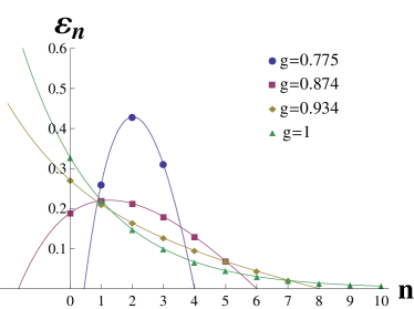
Figure 1: Different representative shapes of the positive spectrum $\varepsilon_{n}$ of the Hermitian operator $\hat{H}_{0}$ for $\alpha=5.1$. The corresponding values of the Gaussianity and purity are $\left(g,\mu\right)=\left\{\left(0.775,0.348\right),\left(0.874,0.183\right),\left(0.934,0.176\right),\left(1,0.196\right)\right\}$

One can see that for all cases the positive spectrum corresponds to  successive number states, so we can conclude that the MSs have the form

$$\hat{\rho}=\sum_{n_{\min}}^{n_{\max}}\varepsilon_{n}^{+}\left|n\right\rangle\left\langle n\right|.$$ (25)

where  $n_{\min}$ and $n_{\max}$ are parameters which also depend on the constraints $\alpha$ and $g$ in a complicated fashion.

III Bounded uncertainty relation

Having identified the form of the MSs we can proceed with the identification of $\lambda_{0}$, $\lambda_{1}$ and $\lambda_{2}$ in Eq.(24) by imposing the constraints of normalization, uncertainty $\alpha$ and Gaussianity $g$. This should be done for all pairs of $n_{\min}$ and $n_{\max}$, but then one should go back and keep only the pairs for which the eigenvalues $\left\{\varepsilon_{n_{\min}},\varepsilon_{n_{\min}},\ldots\varepsilon_{n_{\max}}\right\}$ are positive while all the rest of eigenvalues are negative. Obviously, for some choices of values of uncertainty and Gaussianity no pair of $n_{\min}$ and $n_{\max}$ satisfying these conditions, exists. Otherwise, we can in principle deduce the values of $n_{\min}$ and $n_{\max}$ which are consistent with the constraints of normalization, uncertainty $\alpha$ and Gaussianity $g$. This finally yields the extremal purity $\mu$.

In what follows, we expose one possible way for simplifying this complicated procedure by fixing $n_{\max}$ instead of the Gaussianity $g$. Then we still have to check all values of $n_{\min}$ and keep those that satisfy the positive spectrum condition. The key observation is that if Eq.(24) is re-written substituting the discrete index $n$ by a continuous variable $x$,

$$\lambda_{0}+\lambda_{1}x+\lambda_{2}\frac{2\alpha\left(\alpha-1\right)^{x}}{\left(\alpha+1\right)^{x+1}}$$ (26)

then the zeros of this equation (which are maximum $2$ in number) define  $n_{\min}$  and $n_{\max}$.  More precisely, if the equation has two positive roots, $x_{1}$ and $x_{2}$ ($>x_{1}$), then $n_{\min}=\left\lceil x_{1}\right\rceil$, $n_{\max}=\left\lfloor x_{2}\right\rfloor$ (where $\left\lceil x\right\rceil$ is ceiling function and $\left\lfloor x\right\rfloor$ the floor function). In the case where $x_{1}<0$ or we have only one root $x_{2}>0$ (see yellow curve in 1) then $n_{\min}=0$.  In view of these results, we are able to propose a protocol to obtain in a systematic way the whole set of MSs  where the constraint on the Gaussianity is replaced by a constraint on the second root $x_{2}$ of Eq.(26) which indirectly fixes $n_{\max}$ :

1. Fix  a value for $\alpha>1$, a non-negative integer value for $n_{\min}$ and a real positive value for $x_{2}$ such that $x_{2}-n_{\min}>1$ .

2. Solve the system of equations

   $$\sum_{n=n_{\min}}^{\left\lfloor x_{2}\right\rfloor}\left(\lambda_{0}+\lambda_{1}n+\lambda_{2}\frac{2\alpha\left(\alpha-1\right)^{n}}{\left(\alpha+1\right)^{n+1}}\right)\left(2n+1\right) =\alpha$$ (27)

   $$\sum_{n=n_{\min}}^{\left\lfloor x_{2}\right\rfloor}\left(\lambda_{0}+\lambda_{1}n+\lambda_{2}\frac{2\alpha\left(\alpha-1\right)^{n}}{\left(\alpha+1\right)^{n+1}}\right) =1$$ (28)

   $$\lambda_{0}+\lambda_{1}x_{2}+\lambda_{2}\frac{2\alpha\left(\alpha-1\right)^{x_{2}}}{\left(\alpha+1\right)^{x_{2}+1}} =0$$ (29)

   for $\lambda_{0},$ $\lambda_{1}$, and $\lambda_{2}$ and obtain $\varepsilon_{n}$ from Eq.(24) as a function of $n_{\min}$, $\alpha$ and $x_{2}$. The Eqs.(27)-(28) express the constraints Eq.(6) and Eq.(9) respectively while Eq.(29) ensures that $x_{2}$ is the root of Eq.(26).

3. Verify using the spectrum provided by Eq.(24) that the lowest index of positive part of the spectrum is indeed $n_{\min}$. In other words we check that $\varepsilon_{n_{\min}}\geq 0$ and also that $\varepsilon_{n_{\min}-1}<0$ if $n_{\min}>0$.

This procedure gives the values of the Gaussianity $g$ and the minimum purity $\mu$ corresponding to the chosen parameters $\alpha$ and $x_{2}$, namely

$$g =\sum_{n_{\min}}^{\left\lfloor x_{2}\right\rfloor}\varepsilon_{n}\frac{2\alpha\left(\alpha-1\right)^{n}}{\left(\alpha+1\right)^{n+1}}$$ (30)

$$\mu =\sum_{n_{\min}}^{\left\lfloor x_{2}\right\rfloor}\varepsilon_{n}^{2}.$$ (31)

This yields one MS. To obtain the whole set of MSs this procedure should be repeated by varying the parameters $\alpha$ and $x_{2}$.

According to our studies the above procedure always yields $g<1$, meaning that the derived MSs cannot cover values of $g$ greater than one. For $g=1$ we have the limiting case where $\lambda_{0}=\lambda_{1}=0$, there is no roots for Eq.(29)  and the MSs are the so called ‘thermal’ states (see green curve in Fig.1). For $g>1$ there is no combination of $\lambda$’s which gives positive spectrum solution but by extrapolating the results in PRAr one can construct a bound of minimum purity with the following states

$$\hat{\rho}=r\hat{\rho}_{G}+\left(1-r\right)\left|n\right\rangle\left\langle n\right|$$ (32)

where $n\rightarrow\infty$, $r\rightarrow 1$ while $\mu\left(\hat{\rho}\right)$ is kept constant, and $\hat{\rho}_{G}$ a thermal state

$$\hat{\rho}_{G}=\sum_{m=0}^{\infty}\frac{2\left(\beta-1\right)^{m}}{\left(\beta+1\right)^{m+1}}\left|m\right\rangle\left\langle m\right|$$

of purity $\mu\left(\hat{\rho}_{G}\right)=\frac{1}{\beta}$. The uncertainty $\alpha$ for the MSs in Eq.(32) can be easily calculated

$$\alpha=\frac{g}{\left(2-g\right)\mu},g<1$$ (33)

where $g$  is the Gaussianity   and $\mu$ the purity of the state $\hat{\rho}$.

One may employ the parametric relations Eqs.(30)-(31)  for $g<1$, to represent graphically the surface that stands for the Gaussianity and purity bounded uncertainty relation. For $g>1$ one should employ the much simpler relation given by Eq.(33).  In Fig. 2 we represent the purity and Gaussianity uncertainty relation projected on three, mutually orthogonal planes. One can also see on the same figure the lines which represent the purity bounded uncertainty relation and the Gaussianity bounded one. These one-dimensional uncertainty relations appear as outer boundaries (see red and blue line in Fig. 2) of the surface standing for the purity and Gaussian uncertainty relation. In Fig. 3 we give a $3-$dimensional view of the uncertainty relation.

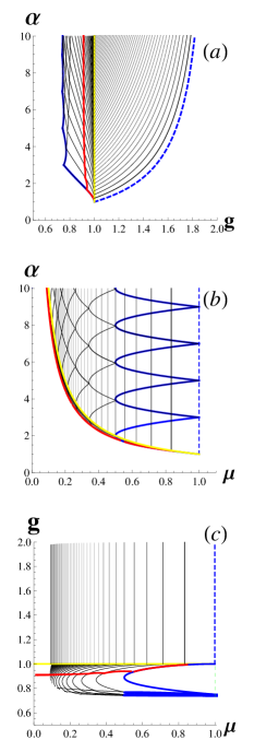
Figure 2: The surface that represents the purity and Gaussianity bounded relation projected on three planes: (a) $\alpha-g$ , (b) $\alpha-\mu$, and (c) $g-\mu$. The red line stands for the purity-bounded uncertainty relation, the blue (dashed and solid) line for the Gaussianity -bounded uncertainty relation and the yellow line for the Gaussian states. For $g>1$ the solid lines are of constant purity (see Eq.(32)). For $g<1$ the surface is separated into segments of MSs with fixed $n_{\min}$ and $n_{\max}$ (see Eq.(25)). The lowest and highest value of uncertainty $\alpha$ for each segment define respectively $n_{\min}$ and $n_{\max}$ according to the relation $\alpha=2n+1$. For the plots we have worked in the domain of uncertainty $1\leq\alpha\leq 10$ and for this reason (c) appears incomplete.

One can observe that the surface representing the uncertainty relation is convex for $g>1$ and its boundaries are laying on the plane of pure states. For $g<1$ a part of the convex surface is somehow “etched” by concave grooves delimited by (blue) loops so that the projections of the loops on $\mu=1$ plane coincide with the intersection of the uncertainty surface with the plane. This reflects the fact that for any given value of $\alpha$ the points of the boundary of the grooves have the same value of $g$ for all available values of $\mu$. Therefore, the curves on the uncertainty surface which correspond to any given $\alpha$ are convex. This convexity makes sufficient our analysis of the states which minimize the purity because we perform it independently for all given values of $\alpha$ and therefore, there is no need to search for the states which maximize the purity.

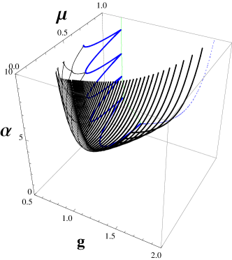
Figure 3: The surface that represents the purity and Gaussianity bounded relation. For a given value of purity $\mu$ and Gaussianity $g$, this surface provides the lowest possible value of the uncertainty $\alpha$ for all quantum states (pure or mixed). The blue line represents the Gaussianity bounded uncertainty relation PRAr .

Not that, the parametric relation for $g<1$ is not very convenient since it is not expressed in the desired form $\alpha\geq f\left(g,\mu\right)$ where for a given value of $g$ and $\mu$ one may conclude on the smallest possible value on the uncertainty $\alpha$. For this reason we have derived the following approximate relation for $f\left(g,\mu\right)$ when $g<1$,

$$f_{\mathrm{app}}\left(g,\mu\right)=\frac{2-g}{g^{7/2}\mu^{g^{2}}}\left(1+\frac{0.2\sqrt{\mu}}{\sqrt{0.01\pi}}\mathrm{e}^{-100(g-0.87)^{2}}\right)^{-1}.$$ (34)

For every pair of values $\left(g,\mu\right)$ it holds that $f\left(g,\mu\right)>$ $f_{\mathrm{app}}\left(g,\mu\right)$ thus the approximate formula provides a lower estimation on the real bound of the uncertainty $f\left(g,\mu\right)$.  In view of these results, we summarize the Gaussianity and purity bounded uncertainty relation as

$$\alpha\geq\left\{\begin{array}[]{cc}\frac{g}{\left(2-g\right)\mu}&,2>g\geq 1\\ f_{\mathrm{app}}\left(g,\mu\right)&,1>g\geq 2/e\end{array}\right\}.$$ (35)

In a previous work SPIE we have derived following a similar but less mathematically consistent method, an uncertainty relation that is bounded by the degree of von Neumann entropy of a state $\hat{\rho}$ and the quantity of overlap $\mathrm{Tr}\left(\hat{\rho}\hat{\rho}_{G}\right)$ between the state and the reference Gaussian state $\hat{\rho}_{G}$. The approach which we follow here, permits us to assert the positivity of the density matrix of the solution in the Lagrange multipliers method while in SPIE we ‘impose’ the positivity on the solution provided by the optimization method. On the other hand, the relation obtained in this work in $3-$dimensional representation, strongly resembles the one in SPIE , with the main difference being on the set of MSs. In SPIE all MSs are of infinite rank while here the rank of the solution (the number of eigenvectors of the solution density matrix) remains finite in the general case ($g\neq 1$).

IV Conclusions

We have introduced and studied an uncertainty relation for the quantum variables of position and momentum, which is tighter than both the Schrödinger-Robertson Robertson and the purity bounded uncertainty relation by Dodonov and Man’ko Man'ko . Our new relation makes the minimum on the uncertainty  $\alpha$ a function of the purity $\mu$ of quantum states and their degree of Gaussianity $g$. Thus the whole  set of quantum states of one-dimensional moving particle (or one optical mode) becomes bounded below in terms of $\alpha$ by a non-trivial surface in three-dimensional parametric space of $\mu$, $g$, and $\alpha$. Being projected on the plane $\mu-\alpha$ our bound recovers the purity bounded uncertainty relation by Dodonov and Man’ko Man'ko while  its projection on the $g-\alpha$ plane recovers the Gaussianity bounded uncertainty relation PRAr . Whereas for $g>1$ our surface is given by an explicit function $\alpha=f\left(g,\mu\right)$ the part of the surface for $g<1$ is obtained only as a parametric function. In order to express our result in the desired form for $g<1$ we have constructed an approximation by function $f_{\mathrm{app}}\left(g,\mu\right)$. This function determines a surface which for any $(g,\mu)$ lays slightly below the actual surface: $f\left(g,\mu\right)>f_{\mathrm{app}}\left(g,\mu\right)$ and thus provides a less tight, but still valid, bound. Finally, our results allow us to visualize the whole set of quantum states in three dimensional parametric space and accurately bound the uncertainty of $x$ and $p$ taking into account the purity and Gaussianity the states for which the uncertainty is evaluated.

Appendix A Appendix

Proposition: The states of minimum purity for given uncertainty and Gaussianity can be expressed as mixtures of number states

Let us consider a general density matrix $\hat{\rho}$ of purity $\mu$ and Gaussianity $g$, whose covariance matrix has been set via LCT proportional to the unity  (in Williamson form) and its displacement vector $\mathbf{d}$ to zero.  In this case the uncertainty $\alpha$ of the state completely characterizes the reference Gaussian state $\hat{\rho}_{G}$ which is just a thermal state. In the Wigner representation   the reference state, $\hat{\rho}_{G}$,

$$W_{G}\left(r\right)=\frac{1}{\pi\alpha}e^{-r^{2}/\alpha},\qquad r=\sqrt{x^{2}+p^{2}}$$ (36)

has no dependence on the angular degree of freedom $\varphi$. In contrast, in the general case the state $\hat{\rho}$ itself possess an angular-dependent Wigner function $W\left(r,\varphi\right)$ and its purity can be expressed via $W\left(r,\varphi\right)$ as

$$\mu=2\pi{\displaystyle\iint}W\left(r,\varphi\right)^{2}r\mathrm{d}r\mathrm{d}\varphi$$ (37)

while its Gaussianity as

$$g=2\pi\alpha{\displaystyle\iint}W\left(r,\varphi\right)W_{G}\left(r\right)r\mathrm{d}r\mathrm{d}\varphi.$$ (38)

The next step is to prove that for any given state $\hat{\rho}$, another state $\hat{\rho}_{s}$ exists of the same $\alpha$ and $g$ and smaller or equal purity, which possess a phase-independent Wigner function. Let us define this new state $\hat{\rho}_{s}$ by phase-averaging the Wigner function $W\left(r,\varphi\right)$ of the initial state $\hat{\rho}$

$$W_{s}\left(r\right)=\frac{1}{2\pi}\int W\left(r,\varphi\right)d\varphi.$$ (39)

Here $W_{s}\left(r\right)$ is the Wigner function of the new state $\hat{\rho}_{s}$. The reference Gaussian state of $\hat{\rho}_{s}$ (and consequently the uncertainty $\alpha$) is the same  as for $\hat{\rho}$, since phase-averaging cannot affect the angular-independent Wigner function Eq.( 36). The Gaussianity degree Eq.(38) remains the same, as well. This is a straightforward result of substitution of the phase-independent Wigner function given by Eq. (39) into Eq. (38). On the other hand, the purity $\mu_{s}$ of the symmetrized state $\hat{\rho}_{s}$ is constrained to be smaller than, or equal to, that of $\hat{\rho}$. Indeed, by applying the Cauchy-Schwarz inequality we have

$$\mu_{s} =2\pi{\displaystyle\iint}W_{s}\left(r\right)^{2}r\mathrm{d}r\mathrm{d}\varphi$$

$$={\displaystyle\iiint}W\left(r,\varphi\right)W\left(r,\Phi\right)r\mathrm{d}rd\varphi d\Phi$$

$$\leq\sqrt{{\displaystyle\iiint}W\left(r,\varphi\right)^{2}r\mathrm{d}rd\varphi d\Phi}\sqrt{{\displaystyle\iiint}W\left(r,\Phi\right)^{2}r\mathrm{d}rd\varphi d\Phi}$$

$$=2\pi{\displaystyle\iint}W\left(r,\varphi\right)^{2}r\mathrm{d}r\mathrm{d}\varphi=\mu.$$

This concludes the proof of this proposition.

From this proposition it is straightforward to deduce that the minimizing states we are looking for, are states of angular-independent Wigner function and therefore can be expressed Werner as a convex combination of the number (Fock) states

$$\hat{\rho}=\sum\rho_{n}\left|n\right\rangle\left\langle n\right|.$$ (40)

References

- (1) E. Schrödinger, Sitzungsber. Preuss. Akad. Wiss. 14, 296 (1930); H. P. Robertson, Phys. Rev. 35, 667A (1930); ibid. 46, 794 (1934).
- (2) V. V. Dodonov, J. Opt. B: Quantum Semiclass. Opt. 4, S98-S108 (2002).
- (3) V. V. Dodonov and V. I. Man’ko, in Invariants and Evolution of Nonstationary Quantum Systems, Proceedings of the Lebedev Physics Institute, Vol. 183, edited by M. A. Markov (Nova Science, Commack, NY, 1989), pp. 4-103.
- (4) M. J. Bastiaans, J. Opt. Soc. Am. A, 1243 (1986).
- (5) A. Mandilara and N. J. Cerf, Phys. Rev. A 86, 030102R (2012).
- (6) A. Mandilara, E. Karpov and N. J. Cerf, Proc. SPIE 7727, 77270H (2010).
- (7) T. Bröckner and R. F. Werner, J. Math. Phys. 36 , 62 (1995).