Omega baryon electromagnetic form factors from lattice QCD

Abstract:

We present results on the Omega baryon ($\Omega^{-}$) electromagnetic form factors using $N_{f}=2+1$ dynamical domain-wall fermion configurations corresponding to a pion mass of about 330 MeV. We construct appropriate sequential sources for the determination of the two dominant form factors $G_{E0}$ and $G_{M1}$ as well as a sequential source that isolates the subdominant electric quadrupole form factor $G_{E2}$. We calculate the $\Omega^{-}$ magnetic moment, $\mu_{\Omega^{-}}$, and electric charge radius, $\langle r^{2}_{E0}\rangle$, and compare to experiment, for the case of $\mu_{\Omega^{-}}$, and to other lattice calculations.

1 Introduction

The structure of hadrons, such as size, shape and charge distribution can be probed by the electromagnetic form factors. The $\Omega^{-}$ baryon, consisting of three valence strange quarks, is significantly more stable than other members of the baryon decuplet, such as the $\Delta$, with a life-time on the order of $10^{-10}s$. This fact makes the calculation of its electromagnetic form factors particularly interesting since they are accessible to experimental measurements. Its magnetic dipole moment is measured to very good accuracy unlike those of the other decuplet baryons. A value of $\mu_{\Omega^{-}}=-2.02(5)$ is given in the PDG [1] in units of nuclear magnetons ($\mu_{N}$). Within lattice QCD one can directly compute hadron form factors starting from the fundamental theory of the strong interactions. Furthermore, higher order multipole moments, not detectable by current experimental setups, are accessible to lattice methods. Higher-order moments such as the electric quadrupole are essential in the determination of the deformation of a hadron state. In this work, we calculate the electromagnetic form factors of the $\Omega^{-}$ baryon using, for the first time, dynamical domain-wall fermion configurations. For the calculation we use the fixed-sink approach which enables us to calculate the form factors for all values and directions of the momentum transfer $\vec{q}$ concurrently. The main advantages of this approach is that it allows an increased statistical precision, while at the same time it provides the full $Q^{2}$ dependence. Moreover, by constructing optimized sources we calculate the two dominant form factors accurately. An appropriately defined source for the subdominant electric quadrupole form factor is constructed and tested [2]. The aim is to obtain an accurate determination of the quadrupole moment, at a price, of course, of additional sequential inversions.

2 Electromagnetic form factors of the $\Omega^{-}$ baryon

The on-shell $\Omega^{-}$ matrix element of the electromagnetic current $j_{EM}^{\mu}$, can be decomposed in terms of four independent Lorentz covariant vertex functions, $a_{1}(q^{2})$, $a_{2}(q^{2})$, $c_{1}(q^{2})$ and $c_{2}(q^{2})$, which depend only on the squared momentum transfer $q^{2}=-Q^{2}=(p_{i}-p_{f})^{2}$. In Minkowski spacetime these are given by [3]

$$\langle\Omega(p_{f},s_{f})|j_{\rm EM}^{\mu}|\Omega(p_{i},s_{i})\rangle=\sqrt{\frac{m^{2}_{\Omega}}{E_{\Omega}(\vec{p_{f}})E_{\Omega}(\vec{p_{i}})}} \,\bar{u}_{\sigma}(p_{f},s_{f}){\cal O}^{\sigma\mu\tau}u_{\tau}(p_{i},s_{i}),$$ (1)

$$\mathcal{O}^{\sigma\mu\tau}=-g^{\sigma\tau}\biggl{[}a_{1}(q^{2})\gamma^{\mu}+\frac{a_{2}(q^{2})}{2m_{\Omega}}\left(p_{f}^{\mu}+p_{i}^{\mu}\right)\biggr{]} -\frac{q^{\sigma}q^{\tau}}{4m_{\Omega}^{2}}\biggl{[}c_{1}(q^{2})\gamma^{\mu}+\frac{c_{2}(q^{2})}{2m_{\Omega}}\left(p_{f}^{\mu}+p_{i}^{\mu}\right)\biggr{]}.$$ (2)

The rest mass and the energy of the particle are denoted by $m_{\Omega}$ and $E_{\Omega}.$ The initial (final) four-momentum and spin-projection are given by $p_{i}\,(p_{f})$ and $s_{i}\,(s_{f})$. In addition, every vector component of the spin-$\frac{3}{2}$ Rarita-Schwinger vector-spinor $u_{\sigma}$ satisfies the Dirac equation, $\big{(}p_{\mu}\gamma^{\mu}-m_{\Omega}\big{)}u^{\sigma}(p,s)=0$, along with the auxiliary conditions: $\gamma_{\sigma}u^{\sigma}(p,s)=0$ and $p_{\sigma}u^{\sigma}(p,s)=0$. Furthermore, the covariant vertex functions are linearly related to the experimentally measured electric $G_{E0}(q^{2})$, $G_{E2}(q^{2})$ and magnetic $G_{M1}(q^{2})$ and $G_{M3}(q^{2})$ multipole form factors  [2, 3].

3 Lattice techniques

We employ gauge configurations generated by the RBC-UKQCD joint collaborations using $N_{f}=2+1$ dynamical domain-wall fermions (DWF) and the Iwasaki gauge-action corresponding to a pion mass of about 330 MeV. The simulation is carried out on a lattice of size $24^{3}\times 64$ with a lattice spacing of 0.114(2) fm. For this pion mass and finite lattice volume the $\Omega^{-}$ is stable. The lattice spacing $a$, the light u and d and the strange quark mass were fixed by an iterative procedure using the $\Omega^{-}$, the pion and the kaon masses [4]. For the present calculations we use 200 well separated dynamical domain-wall fermion gauge configurations [4]. It is known that the chiral symmetry breaking falls exponentially with the length of the fifth dimension $N_{5}$ of the DWF-action. The value $N_{5}=16$ used here is adequate to keep the residual mass sufficiently small.

3.1 Interpolating fields

In order to calculate the $\Omega^{-}$ matrix element we need to evaluate the appropriate two- and three-point correlation functions. An interpolating field operator with the quantum numbers of the $\Omega^{-}$ hyperon is given by

$$J_{\Omega}(x) =\epsilon^{abc}\,\mathbf{s}^{a}_{\alpha}\,\big{(}\mathbf{s}^{\!\mbox{\tiny T}b}_{\beta}\,[C\gamma_{\sigma}]_{\beta\gamma}\,\mathbf{s}^{c}_{\gamma}\big{)},$$ (3)

where $C=\gamma_{4}\gamma_{2}$ is the charge-conjugation matrix and $\sigma$ is the vector index of the spin-3/2 spinor.

In order to ensure ground state dominance for the shortest time evolution we perform a gauge invariant Gaussian smearing, as described in Refs. [5, 6], on the quark fields $\mathbf{s}$ that enter in the interpolating field:

$${\mathbf{q}}_{\beta}(t,\vec{x})=\sum_{\vec{y}}[\mathds{1}+\alpha H(\vec{x},\vec{y};U)]^{n}\ q_{\beta}(t,\vec{y}),$$

$$H(\vec{x},\vec{y};U)=\sum_{\mu=1}^{3}\left(U_{\mu}(\vec{x},t)\delta_{\vec{x},\vec{y}-\hat{\mu}}+U^{\dagger}_{\mu}(\vec{x}-\hat{\mu},t)\delta_{\vec{x},\vec{y}+\hat{\mu}}\right),$$

where $\mathbf{q}$ (q) is the smeared (local) fermion field. The links $U_{\mu}(\vec{x},\,t)$ entering the hopping matrix $H$ are APE-smeared gauge fields.

Figure 1: The $\Omega^{-}$ effective mass and the fit to the plateau plotted against time separation.

For the lattice spacing considered here we have used the Gaussian smearing parameters $\alpha=5.026$ and $n=40$, which have been optimized for the nucleon state. In Fig. 1 we show the $\Omega^{-}$ effective mass, calculated from the two-point function ratio defined by $m_{eff}^{\Omega}(t)=-\log[G(t+1,{\vec{0}})/G(t,\vec{0})]$. It displays a nice plateau yielding $m_{\Omega}=1.76(2)\ \mathrm{GeV}$. This value is 5% higher than the experimental one. This may reflect a slightly larger value for the strange quark mass as compared to the physical one.

3.2 Two- and three-point Correlation functions

The electromagnetic form factors are extracted by constructing appropriate combinations of two- and three-point correlation functions. The corresponding lattice correlation functions are given by

$$G(t_{f},\vec{q}) =\sum_{\vec{x}_{f}}\sum_{j=1}^{3}e^{-i\vec{x}_{f}\cdot\vec{q}}\,\Gamma^{4}_{\alpha\beta}\langle J_{j\beta}(x_{f})\overline{J}_{j\alpha}(0)\rangle,$$ (4)

$$G^{\ \mu}_{\sigma\ \tau}(\Gamma^{\nu},t,\vec{q}) =\sum_{\vec{x}_{f}\vec{x}}e^{i\vec{x}\cdot\vec{q}}\Gamma^{\nu}_{\alpha\beta}\langle J_{\sigma\beta}(x_{f})j_{EM}^{\mu}(x)\overline{J}_{\tau\alpha}(0)\rangle,$$ (5)

where $\Gamma^{4}=\frac{1}{4}\big{(}\mathds{1}+\gamma^{4}\big{)}$ and $\Gamma^{k}=i\Gamma^{4}\gamma^{5}\gamma^{k}$, with the Dirac $\gamma$-matrices taken in Euclidean spacetime. We calculate the above three-point correlation function in a frame where the final $\Omega^{-}$ state is at rest, $\vec{p}_{f}=\vec{0}$, while the operator $j^{\mu}_{EM}$ is inserted at time $t$ carrying a momentum $\vec{q}=-\vec{p}_{i}$.

The leading time dependence and unknown overlaps of the $\Omega^{-}$ state with the initial state $\bar{J}_{\Omega}|0\rangle$ in the three-point correlation function can be canceled out by forming appropriate ratios of the three-point function and two-point functions. A particularly suitable ratio is defined by

$$R_{\sigma\ \tau}^{\ \mu}(\Gamma,\vec{q},t) =\frac{G_{\sigma\ \tau}^{\ \mu}(\Gamma^{\nu},\vec{q},t)}{G_{kk}(\Gamma^{4},\vec{0},t_{f})}\ \sqrt{\frac{G_{kk}(\Gamma^{4},\vec{p}_{i},t_{f}-t)G_{kk}(\Gamma^{4},\vec{0},t)G_{kk}(\Gamma^{4},\vec{0},t_{f})}{G_{kk}(\Gamma^{4},\vec{0},t_{f}-t)G_{kk}(\Gamma^{4},\vec{p}_{i},t)G_{kk}(\Gamma^{4},\vec{p}_{i},t_{f})}}\,,$$ (6)

where a summation over the repeated indices $k\,\,(k=1,2,3)$ is assumed. For large Euclidean time separations this ratio becomes time-independent (plateau region)

$$R_{\sigma\ \tau}^{\ \mu}(\Gamma,\vec{q},t)\stackrel{{\scriptstyle t_{f}-t\gg 1,t\gg 1}}{{\longrightarrow}}\Pi_{\sigma\ \tau}^{\ \mu}(\Gamma,\vec{q}) =\mathcal{C}\ \mathrm{Tr}\left[\Gamma\,\Lambda_{\sigma\sigma}(p_{f})\mathcal{O}^{{\sigma}\mu{\tau}}\Lambda_{\tau\tau}(p_{i})\right],$$ (7)

$$\mathcal{C} =\sqrt{\frac{3}{2}}\left[\frac{2E_{\Omega}(\vec{q})}{m_{\Omega}}+\frac{2E^{2}_{\Omega}(\vec{q})}{m^{2}_{\Omega}}+\frac{E^{3}_{\Omega}(\vec{q})}{m^{3}_{\Omega}}+\frac{E^{4}_{\Omega}(\vec{q})}{m^{4}_{\Omega}}\right]^{-\frac{1}{2}}.$$ (8)

It is understood that the trace acts on spinor-space, while the Euclideanized version of the Rarita-Schwinger spin sum is given by

$$\Lambda_{\sigma\tau}(p) \equiv\sum_{s}u_{\sigma}(p,s)\bar{u}_{\tau}(p,s)=-\frac{-i\not{p}+m_{\Omega}}{2m_{\Omega}}\left[\delta_{\sigma\tau}-\frac{\gamma_{\sigma}\gamma_{\tau}}{3}+\frac{2p_{\sigma}p_{\tau}}{3m_{\Omega}^{2}}-i\frac{p_{\sigma}\gamma_{\tau}-p_{\tau}\gamma_{\sigma}}{3m_{\Omega}}\right]\,.$$ (9)

The electromagnetic form factors are extracted by fitting to the plateau region of a set of specially chosen combinations of three-point functions given below

$$\sum_{k=1}^{3}\Pi_{k\ k}^{\ \mu}(\Gamma^{4},\vec{q}) =K_{1}\ G_{E0}(Q^{2})+K_{2}\ G_{E2}(Q^{2}),$$ (10)

$$\sum_{j,k,l=1}^{3}\epsilon_{jkl}\Pi_{j\ k}^{\ \mu}(\Gamma^{4},\vec{q}) =K_{3}\ G_{M1}(Q^{2}),$$ (11)

$$\sum_{j,k,l}^{3}\epsilon_{jkl}\Pi_{j\ k}^{\ 4}(\Gamma^{j},\vec{q}) =K_{4}\ G_{E2}(Q^{2}).$$ (12)

The continuum kinematical coefficients $K_{i}\ \ (i=1,2,3,4),$ have been calculated in Ref. [7] and are functions of the $\Omega^{-}$ mass, the energy $E_{\Omega}$, the space-time index $\mu$ and the momentum $\vec{q}$. Furthermore, it is readily seen that the subdominant electric quadrupole form factor $G_{E2}$ is isolated by the combination provided by Eq. (12). In addition, these expressions are such that all possible directions of $\mu$ and momentum $\vec{q}$ contribute in a symmetric fashion at a given momentum transfer $Q^{2}.$ In other words, the optimal combinations of $\Pi_{\sigma\ \tau}^{\ \mu}(\Gamma,\vec{q})$ employed are those that maximize the number of nonzero $\vec{q}$ contributions in a lattice rotationally invariant way [8].

We calculate only the connected contributions to the three-point function by performing sequential inversions through the sink. This means that we need to fix the quantum numbers of the initial and final states and explains why we consider optimal combinations. Otherwise, one would have to prepare a new set of sequential inversions for every choice of vector and Dirac indices, which is prohibited in a lattice computation given the fact that we have to consider an overall of $\sigma\times\beta\times\tau\times\alpha=256$, combinations by looking the index structure of Eq. (5). Having the matrix element for all the different directions of $\vec{q}$ and for all four directions $\mu$ of the current, we form an over-constrained system of linear equations (in terms of form factors), which is solved by employing a singular value decomposition analysis. This procedure yields the electromagnetic form factors $G_{E0}$, $G_{M1}$ and $G_{E2}$. The statistical errors are found by a jack-knife analysis, which takes care of the correlations of lattice measurements of the ratios.

As already mentioned the three-point function of the connected part is calculated by performing sequential inversions through the sink. This requires to fix the temporal source-sink separation. In order to determine the smallest time separation that is still sufficiently large to damp the excited state contributions we perform the calculation at two values of the sink-source separation, namely $t_{f}/a=8$ and $t_{f}/a=10$. We compare in Fig. 2 the results for the plateaus $\Pi_{\sigma\ \tau}^{\ \mu}(\Gamma,\vec{q})$, for a few selected directions of the current and for low momentum $\vec{q}$ values for these two sink-source time separations. As can be seen, the plateaus values at $t_{f}/a=10$ are consistent with the smaller time separation having about half the statistical error. We therefore use $t_{f}/a=8$ or $t_{f}=0.91$ fm in what follows.

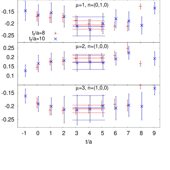
Figure 2: The ratio $R_{\sigma\ \tau}^{\ \mu}(\Gamma,\vec{q},t)$ extracted for temporal source-sink separations $t_{f}/a=8$ and $t_{f}/a=10$, using 50 gauge configurations. The results for $t_{f}/a=10$ are shifted to the left by one unit. We show results for current directions $\mu=1,2,3$ and low-momenta $\vec{q}$: $(0,1,0)\frac{2\pi}{L}$ and $(1,0,0)\frac{2\pi}{L}$, respectively.

4 Results

We use the local electromagnetic current, $j_{EM}^{\mu}=-\frac{1}{3}\bar{s}\gamma^{\mu}s$, which requires a renormalization factor $Z_{V}$ to be included. This renormalization constant is determined by the requirement that $G_{E0}$ at zero momentum transfer is equal to the charge of $\Omega^{-}$ in units of electric charge, that is $G_{E0}(0)\equiv-1$. Our calculation, at this quark mass, yields a value of $Z_{V}=0.727(1)$, which is reasonably close to the value obtained in Refs. [9, 4] in the chiral limit.

4.1 Electric charge form factor

Our results for the electric charge form factor, $G_{E0}$, are depicted in Fig. 3(a). As can be seen, the momentum dependence of this form factor is described well by a dipole form

$$G_{E0}(Q^{2}) =-\frac{1}{\big{(}1+\frac{Q^{2}}{\Lambda_{E0}^{2}}\big{)}^{2}},$$ (13)

with $\Lambda_{E0}^{2}$ a fit parameter. In the non-relativistic limit the slope of the above dipole form evaluated at momentum transfer $Q^{2}=0$, is related to the electric charge root mean square (rms) radius

$$\left\langle r^{2}_{E0}\right\rangle=-6\frac{d}{dQ^{2}}G_{E0}(Q^{2})\bigg{|}_{Q^{2}=0}\,.$$ (14)

From our dipole fit to the lattice data we determine $\Lambda_{E0}$ and obtain a value of $\langle r^{2}_{E0}\rangle=-0.354(9)\ \mathrm{fm}^{2}$. This is slightly greater in magnitude than the one reported in Ref. [10], which was obtained in a quenched lattice QCD calculation (see Table 1). Our value is expected to be higher since in a dynamical lattice calculation meson-cloud effects are taken into account in addition to the fact that in Ref. [10] a heavy pion mass has been used.

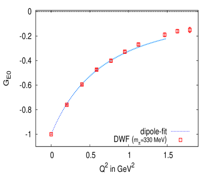
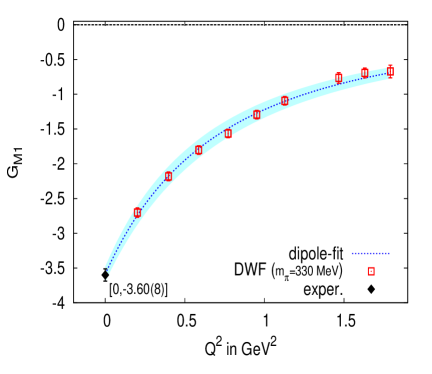
(a)	(b)

Figure 3: (a) The electric charge form factor $G_{E0}$ at $m_{\pi}=330\ \mathrm{MeV}.$ The line describes the dipole fit given in Eq. (13). (b) The magnetic dipole form factor, $G_{M1}$, along with the dipole fit as given in Eq. (15) at $m_{\pi}=330\ \mathrm{MeV}$. The experimental datum for the magnetic dipole form factor, $G_{M1}(0)=-3.60(8)\ \mathrm{GeV}^{2}$ [1], is also shown.

4.2 Magnetic dipole form factor

Lattice results on the magnetic dipole $G_{M1}$ are shown in Fig. 3(b). As in the case of $G_{E0}$, a dipole fit describes very well the $Q^{2}$-dependence of $G_{M1}$. Fitting to the form

$$G_{M1}(Q^{2})=-\frac{G_{M1}(0)}{\big{(}1+\frac{Q^{2}}{\Lambda_{M1}^{2}}\big{)}^{2}}$$ (15)

we can extract the anomalous magnetic moment of the $\Omega^{-}$. By utilizing the lattice computed $\Omega$ mass, from Table 1, we calculate the magnetic moment in nuclear magnetons by using the relation

$$\mu_{\Omega^{-}} =G_{M1}(0)\frac{e}{2m_{\Omega}}=G_{M1}(0)\ \frac{m_{N}}{m_{\Omega}}\ \mu_{N}.$$ (16)

Our value of $\mu_{\Omega^{-}}$ in nuclear magnetons $\mu_{N}$ is given in Table 1 and it is in agreement with the experimental value. It is also in agreement with two recent lattice calculations [10, 11]. The calculation in Ref. [10] is similar to ours in the sense that the three-point correlation function is calculated but the evaluation is carried out in the quenched theory and only at one value of $Q^{2}$. In Ref. [11] one employs a background field method to compute energy shifts using $N_{F}=2+1$ Clover fermions at pion mass of 366 MeV on an anisotropic lattice.

	Vol.	$N_{\mathrm{conf.}}$	$m_{\pi}$	$m_{\Omega}$	$G_{M1}(0)$	$\mu_{\Omega^{-}}$	$\langle r^{2}_{E0}\rangle$
			[MeV]	[GeV]	[$\mathrm{GeV}^{2}$]	[$\mu_{N}$]	[$\mathrm{fm}^{2}$]
this work	$24^{3}\times 64$	200	330	1.763(21)	-3.58(10)	-1.92(6)	-0.354(9)
ref. [10]	$20^{3}\times 40$	400	697	1.732(12)	–	-1.697(65)	-0.307(15)
ref. [11]	$24^{3}\times 128$	213	366	1.650	–	-1.93(8)	–
ref. [1] [PDG]	–	–	–	1.672(45)	-3.60(8)	-2.02(5)	–

Table 1: The $\Omega^{-}$ mass $m_{\Omega}$, the magnetic dipole form factor $G_{M1}$ at $Q^{2}=0$, the magnetic moment $\mu_{\Omega^{-}}$ and the electric rms charge radius $\langle r^{2}_{E0}\rangle$.

5 Summary

Using appropriately constructed sequential sources the dominant $\Omega^{-}$ electromagnetic form factors $G_{E0}$ and $G_{M1}$ are calculated with good accuracy even with a small sample of dynamical domain-wall fermion configurations. In the current calculation we neglected disconnected contributions.

The $\Omega^{-}$ magnetic moment is extracted by fitting the magnetic dipole form factor $G_{M1}$ to a dipole form. We find a value that is in agreement with experiment [1]. The electric rms charge radius $\langle r^{2}_{E0}\rangle$ is also computed and found to be larger than the value obtained in quenched QCD [10].

We have also preliminary results on the subdominant electric quadrupole form factor $G_{E2}$ using the source of Eq. (12) but with our current statistics the errors are still large and no definite conclusion can be drawn.

We will check for cut-off effects by performing the calculation of the form factors using dynamical domain-wall fermion configurations at a finer lattice spacing. Although the light quark mass dependence is expected to be small, this needs to be checked at another, preferably smaller, value of the pion mass.

References

• [1] C. Amsler et al. (Particle Data Group), PL B667 (2008) 1.
• [2] C. Alexandrou et al., Phys. Rev.  D 79 (2009) 014507.
• [3] S. Nozawa and D. B. Leinweber, Phys. Rev.  D 42 (1990) 3567.
• [4] C. Allton et al. [RBC-UKQCD Collaboration], Phys. Rev.  D 78 (2008) 114509.
• [5] C. Alexandrou, S. Gusken, F. Jegerlehner, K. Schilling and R. Sommer, Nucl. Phys.  B 414 (1994) 815.
• [6] M. Albanese et. al. (APE Collaboration) Phys.  Lett.  B 192 (1987) 163.
• [7] C. Alexandrou et al., Nucl. Phys.  A 825 (2009) 115.
• [8] C. Alexandrou, G. Koutsou, H. Neff, J. W. Negele, W. Schroers and A. Tsapalis, Phys. Rev.  D 77 (2008) 085012.
• [9] Y. Aoki et al., Phys. Rev.  D 78 (2008) 054510.
• [10] S. Boinepalli, D. B. Leinweber, P. J. Moran, A. G. Williams, J. M. Zanotti and J. B. Zhang, Phys. Rev. D 80, 054505 (2009), arXiv:0902.4046 [hep-lat].
• [11] C. Aubin, K. Orginos, V. Pascalutsa and M. Vanderhaeghen, Phys. Rev. D 79, 051502 (2009), arXiv:0811.2440 [hep-lat].
• [12] D. B. Leinweber, T. Draper and R. M. Woloshyn, Phys. Rev.  D 46 (1992) 3067.