Scanning tunneling spectroscopic evidence of crossover transition
in the two-impurity Kondo problem

Abstract

We calculate the differential conductance (dI/dV) corresponding to scanning tunneling spectroscopy (STS) measurements for two magnetic atoms adsorbed on a metal surface with the aid of the numerical renormalization group (NRG) technique. We find that the peak structure of the dI/dV spectra near the Fermi level changes gradually as a function of the adatom separation and the coupling between the adatoms and the metal surface conduction band. When the coupling becomes small, the peak disappears and, instead, a dip structure appears near the Fermi level. This dip structure is the manifestation of the strong antiferromagnetic correlation between the localized spins. The gradual change of the dI/dV structure from a peak structure to a dip structure originates from the crossover transition in the two impurity Kondo problem.

I Introduction

The two-impurity Kondo problem has long been extensively investigated. Generally, the low temperature physics depends on the ratio between the RKKY coupling constant $J_{\mathrm{RKKY}}$ and the one-impurity Kondo temperature $T_{\mathrm{K}}$ Jayaprakash et al. (1981). In the limit of strong ferromagnetic RKKY coupling ($-J_{\mathrm{RKKY}}>>T_{\mathrm{K}}$), a two stage Kondo effect occurs: First the localized spins are partially compensated as temperature $T$ decreases, and then completely suppressed as $T$ goes to zero. In the limit of strong antiferromagnetic RKKY coupling ($J_{\mathrm{RKKY}}>>T_{\mathrm{K}}$), the localized spins are locked into a spin-singlet state (the antiferromagnetic region), and the Kondo effect plays a minor role. In the $T_{\mathrm{K}}>>|J_{\mathrm{RKKY}}|$ region (the Kondo region), the RKKY interaction plays a minor role.
  The scenarios in the corresponding limits are very reasonable, but the physics in the region at intermediate values of $J_{\mathrm{RKKY}}$ is nontrivial. Studies carrying out numerical renormalization group (NRG) diagonalization on the electron-hole (e-h) symmetric Hamiltonian found a critical point which separates the Kondo region and the antiferromagnetic region Jones et al. (1988); Jones and Varma (1989). However, it is now apparent that the critical point results from the e-h symmetry of the model HamiltonianAffleck et al. (1995); Sakai and Shimizu (1992a). In general, e-h symmetry is broken (e.g., energy dependence in tunneling matrix elements) and the quantum phase transition is replaced by a crossover transition Silva et al. (1996).
  The magnetic atom dimer on a nonmagnetic metal surface is a classical example of a two-impurity Kondo system. In this system, the strength and sign of the RKKY interaction can be adjusted by changing the adatom separation. Using STS, the Kondo effect can be observed through the sharp peak structure near Fermi level, which corresponds to the Yosida-Kondo singlet Kasai et al. (2000); Kawasaka et al. (1999); Shimada et al. (2003); Di$\mathrm{\tilde{n}}$o et al. (2006); Madhavan et al. (1998); Heinrich et al. (2004); Crommie et al. (1993); Minamitani et al. (2009a, b). Thus, we would expect to observe the interference between the Kondo effect and the spin ordering effect of the RKKY interaction through the STS spectra. Experimentally, the STS spectra of a Co dimer on a Cu(100) surface vary with the change of the adatom separation Wahl et al. (2007), which is expected to result from the two impurity Kondo problem. However, theoretical studies specific to STS measurements are rareMinamitani et al. (2009a, b); Merino et al. (2009b). In our earlier studies, we confirmed that the ferromagnetic (antiferromagnetic) interaction tends to sharpen (broaden) the dI/dV peak structure Minamitani et al. (2009a, b). On the other hand, we find from dI/dV calculations based on e-h symmetric Hamiltonian that such a broad peak does not exist. These results indicate that the observed broad STS spectra are related to the crossover between the Kondo region and the antiferromagnetic region.
  Both $T_{K}$ and $J_{RKKY}$ strongly depend on the ratio between the Coulomb interaction $U$ and the coupling between the adatom and the metal surface conduction band, $\Gamma$. As schematically shown in Fig.1, $T_{K}$ decays much faster than $J_{RKKY}$ as $\Gamma$ decreases.

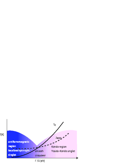
Figure 1: Diagram of the smooth crossover in the two impurity Kondo effect. $T$ is the temperature. $T_{K}$ is the Kondo temperature and $J_{RKKY}$ is the RKKY coupling constant.

With small $\Gamma$, we would expect that the antiferromagnetic RKKY interaction becomes dominant. In this situation, adjusting the RKKY interaction by changing the adatom separation, we can trace the crossover between the Kondo region and the antiferromagnetic region. For this reason, we calculate the dI/dV spectra for several values of $\Gamma$ and the adatom separation to show how the crossover transition in the two impurity Kondo problem can be observed through the STS spectra.

II Model and Method

As experiments showHeinrich et al. (2004); Otte et al. (2008), by covering the metal surface with a decoupling layer, $\Gamma$ was suppressed, which leads to a decrease in $T_{K}$. In the present study, we consider the model system shown in Fig.2.

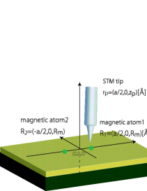
Figure 2: STS observation of a magnetic dimer on a nonmagnetic metal surface. Distances between the adatoms ($a$) , the tip apex and the metal surface ($z_{p}$) are given in Ångströms [Å]. STM tip is placed directly above atom 1.

Magnetic atom 2 is located at a distance of $a$ Å  with respect to magnetic atom 1. We assume that the center of atom 1 is located at $\mathbf{R_{1}}=(a/2,0,R_{m})$ Å  and that of atom 2 is located at $\mathbf{R_{2}}=(-a/2,0,R_{m})$ Å. $R_{m}$ is the radius of adatom. We set $R_{m}=0.4$ Å Shimada et al. (2003). The tip apex is at a distance of $z_{p}$ from the metal surface, directly above atom 1. $R_{o}$ is the thickness of the decoupling layer and we set $R_{o}=5$Å. The corresponding model Hamiltonian is given by

$$H = H_{A2}+H_{tip}+H_{mix}$$ (1)

$$= \sum_{i\sigma}E_{d}d_{i\sigma}^{\dagger}d_{i\sigma}+\sum_{k,\sigma}E_{k}c_{k\sigma}^{\dagger}c_{k\sigma}+\sum_{ik\sigma}(V_{kdi}c_{k\sigma}^{\dagger}d_{i\sigma}+h.c.)$$

$$+\sum_{i}Un_{i\uparrow}n_{i\downarrow}+\sum_{p,\sigma}E_{p}c^{\dagger}_{p\sigma}c_{p\sigma}$$

$$+\sum_{li\sigma}(T_{pdi}c_{p\sigma}^{\dagger}d_{i\sigma}+h.c.)+\sum_{pk\sigma}(W_{pk}c_{p\sigma}^{\dagger}c_{k\sigma}+h.c.).$$

Here $d_{i\sigma}^{\dagger}$, $c_{k\sigma}^{\dagger}$ and $c^{\dagger}_{p\sigma}$ correspond to creation operators for adatom $d$ electrons, metal surface conduction electrons, and tip electrons with spin $\sigma$, respectively. $n_{i\sigma}=d^{\dagger}_{i\sigma}d_{i\sigma}$. $E_{d}$, $E_{k}$ and $E_{p}$ correspond to the kinetic energies of adatom $d$ electrons, conduction electrons and tip electrons, respectively. Adatom index $i=1,2$. $k$ corresponds to the metal surface electron wavenumber, and $p$ corresponds to eigenstate quantum number of the tip electrons. $T_{pdi}$, $W_{pk}$, and $V_{kdi}$ correspond to the tip-adatom, tip-surface, and adatom-surface electron tunneling matrix elements, respectively. $U$ gives the on-site Coulomb repulsion on adatoms. We approximate the coefficients in the Hamiltonian (1) as

$$V_{kd1} = V_{0}\exp(i\mathbf{k}\cdot a/2),V_{kd2}=V_{0}\exp(-i\mathbf{k}\cdot a/2),$$ (2)

$$W_{kp} = W_{0}\exp(-(z_{p}-R_{s}+R_{o})/\lambda)\exp(-i(\mathbf{k\cdot r_{p}})),$$

$$T_{pdi} = T_{0}\frac{\psi_{di}(\mathbf{r_{p}}-\mathbf{R_{i}})}{\psi_{di}(\mathbf{R_{i}}+\mathbf{R})}=T_{0}\Phi_{di},$$ (4)

and

$$\Phi_{di}=\frac{\psi_{di}(\mathbf{r_{p}}-\mathbf{R_{i}})}{\psi_{di}(\mathbf{R_{i}}+\mathbf{R})}.$$ (5)

$\psi_{di}$ corresponds to the $d$ electron orbital of adatom $i$. We approximate the tip apex as a nonmagnetic metal sphere whose center is positioned at $\mathbf{r_{p}}=(a/2,0,z_{p})$ with radius $Rs$. $\mathbf{R}=(0,0,Rs)$ and $\mathbf{a}=(a,0,0)$. $W_{0}$ and $T_{0}$ correspond to the values of the tunneling matrix elements when the tip is in contact with the surface or adatoms, respectively. $V_{0}$ is the tunneling matrix element between a localized d electron and a metal surface in the single impurity case.

Using non-equilibrium Green’s function methodShimada et al. (2003); Rammer and Smith (1986), the electron current from the STM tip to the surface can be written as

$$I = \frac{2e}{h}\sum_{\sigma}\int d\omega(f_{k}-f_{p})\Bigl{\{}2\pi T_{0}^{2}(\Phi_{d1}^{2}+\Phi_{d2}^{2})\rho_{p}\Im G_{11\sigma}^{r}$$ (6)

$$+ 4\pi T_{0}^{2}\Phi_{d1}\Phi_{d2}\rho_{p}\Im G_{12\sigma}^{r}-2\pi^{2}\rho_{k}\rho_{p}W_{0}^{2}e^{-2(z_{p}-R_{s})/\lambda}$$

$$- 4\pi T_{0}(\Phi_{d1}J_{vw}(r_{1})+\Phi_{d2}J_{vw}(r_{2}))\rho_{p}\Re G_{11\sigma}^{r}$$

$$- 4\pi T_{0}(\Phi_{d1}J_{vw}(r_{2})+\Phi_{d2}J_{vw}(r_{1}))\rho_{p}\Re G_{12\sigma}^{r}$$

$$- 2\pi(J_{vw}^{2}(r_{1})+J_{vw}^{2}(r_{2}))\rho_{p}\Im G_{11\sigma}^{r}$$

$$- 4\pi J_{vw}(r_{1})J_{vw}(r_{2})\rho_{p}\Im G_{12\sigma}^{r}\Bigr{\}}.$$

From Eq. (6) we can then obtain the corresponding differential conductance $dI/dV$. In Eq. (6), the retarded Green’s function $G_{ij\sigma}^{r}$ of the surface system corresponds to that of the two-impurity Anderson model. $f_{k}$ and $f_{p}$ give the Fermi distribution functions for the surface and tip, respectively. $\rho_{k}$ and $\rho_{p}$ give the density of states of the conduction electrons and the STM tip electrons, respectively. We define $\Phi_{di}$ and $J_{vw}(r)$ as follows -

$$J_{vw}(r) = \pi\rho_{k}J_{0}(k_{F}r)V_{0}W_{0}\exp(-(z_{p}-R_{s}+R_{o})/\lambda).$$

$\lambda$ is the decay constant of the surface electron wave function. $J_{0}$ is the 0th order Bessel function. Using these parameters, $\Gamma$ is defined as $\Gamma=\pi\rho_{k}V_{0}^{2}$. At $T=0$ K, $dI/dV$ can be rewritten in the following simplified form -

$$dI/dV(eV) \propto A_{11}\Im G_{11\sigma}^{r}(eV)+A_{12}\Im G_{12\sigma}^{r}(eV)$$ (8)

$$+ B_{11}\Re G_{11\sigma}^{r}(eV)+B_{12}\Re G_{12\sigma}^{r}(eV)$$

Coefficients such as $A_{11},B_{11}$ can be derived from the coefficients of the Green’s function in Eq. (6), i.e.,

$$A_{11} = -2\pi T_{0}^{2}(\Phi_{d1}^{2}+\Phi_{d2}^{2})\rho_{p},$$ (9)

$$+ 2\pi(J_{vw}^{2}(r_{1})+J_{vw}^{2}(r_{2}))\rho_{p},$$

$$A_{12} = -4\pi T_{0}^{2}\Phi_{d1}\Phi_{d2}\rho_{p}+4\pi J_{vw}(r_{1})J_{vw}(r_{2})\rho_{p},$$ (10)

$$B_{11} = 4\pi T_{0}(\Phi_{d1}J_{vw}(r_{1})+\Phi_{d2}J_{vw}(r_{2}))\rho_{p},$$ (11)

$$B_{12} = 4\pi T_{0}(\Phi_{d1}J_{vw}(r_{2})+\Phi_{d2}J_{vw}(r_{1}))\rho_{p}.$$ (12)

The third and fourth terms are related to the Fano effect and makes the $dI/dV$ spectra asymmetric. We show several values of each coefficient eq.(8) in the case of $\Gamma=0.022$eV at several adatom separation in Table 1 .

Table 1: Values of coefficients in Eq.(8) in the case of $\Gamma=0.022$ eV at several adatom separations ($a$).

$a$ (Å)	$A_{11}$ (eV)	$A_{12}$ (eV)	$B_{11}$ (eV)	$B_{12}$ (eV)
5.0	-6.6225$\times 10^{-4}$	-1.6792$\times 10^{-9}$	5.3360$\times 10^{-7}$	1.7792$\times 10^{-7}$
6.0	-6.6225$\times 10^{-4}$	6.8125$\times 10^{-10}$	5.3360$\times 10^{-7}$	6.6775$\times 10^{-8}$
7.0	-6.6225$\times 10^{-4}$	2.9035$\times 10^{-11}$	5.3360$\times 10^{-7}$	-3.5216$\times 10^{-8}$
8.0	-6.6225$\times 10^{-4}$	-4.6240$\times 10^{-11}$	5.3360$\times 10^{-7}$	-1.1929$\times 10^{-7}$
9.0	-6.6225$\times 10^{-4}$	-7.1997$\times 10^{-11}$	5.3360$\times 10^{-7}$	-1.7886$\times 10^{-7}$

As can be seen from Table 1, in eq.(8), $A_{11}\Im G_{11\sigma}^{r}(eV)$ is dominant and other parts play only minor roles. This means that the decoupling layer suppresses the Fano effect. To derive the relevant Green’s function, we adopt the NRG technique Krishna-murthy et al. (1980a, b); Sakai and Shimizu (1992a); Campo et al. (2005); Bulla et al. (2008). In the present study, we transform $H_{A2}$ in eq.(1) into two semi-infinite chains form so as to be suitable for NRG calculation Campo et al. (2005); Silva et al. (1996); Minamitani et al. (2009a, b):

$$H_{A2} = \sum_{nq=\pm}\epsilon_{nq}f^{\dagger}_{nq}f_{nq}+\sum_{nq=\pm}(t_{nq}f^{\dagger}_{nq}f_{n+1q}+H.c.)$$ (13)

$$+ \sum_{q=\pm}E_{d}n_{dq}+U\sum_{i=1,2}n_{di\uparrow}n_{di\downarrow}$$

$$+ \sqrt{\frac{2D\Gamma}{\pi}}\sum_{q=\pm}(\sqrt{\bar{\gamma}}f^{\dagger}_{0q}d_{q}+h.c.).$$

Here, $f_{nq}$ corresponds to the $n$th site of the conduction electron part of the chain (Wilson chain) with the parity $q$. $q=+,-$ denotes the even and odd parity states, respectively. $d_{+}=\frac{d_{1}+d_{2}}{\sqrt{2}}$ and $d_{-}=\frac{d_{1}-d_{2}}{\sqrt{2}}$. $D$ gives the conduction electron band width. $\epsilon_{nq}$ and $t_{nq}$ are the corresponding matrix elements for the Wilson chain. When the metal surface conduction band is that for a two dimensional free electron,

$$f_{0\pm} = \int^{D}_{-D}\sqrt{\gamma_{\pm}(\epsilon)}c_{\epsilon\pm}/\sqrt{\bar{\gamma_{\pm}}}d\epsilon,$$ (14)

$$\gamma_{\pm}(\epsilon) = \frac{1\pm J_{0}(ka)}{2},$$ (15)

$$\bar{\gamma_{\pm}} = \int^{D}_{-D}\gamma_{\pm}(\epsilon)d\epsilon.$$ (16)

III Numerical results and Discussions

The two dominant parameters $T_{K}$ and $J_{RKKY}$ strongly depend on the value of $\Gamma$. $T_{K}$ decays much faster than $J_{RKKY}$ as $\Gamma$ decreases. The values of $\Gamma$ (therefore $T_{K}$) depend on the thickness, the surface condition and the type of the decoupling layer. In the present study, we set the thickness of the decoupling layer to 5Å Heinrich et al. (2004). In such system, the value of $T_{K}$ ranges from 3 to 6K. Thus, we calculate the dI/dV spectra with $\Gamma=0.025,0.022$, and $0.02$eV at several adatom separations. (From Yoshimori and Kasai (1986), corresponding $T_{K}$ is estimated at 6.64, 3.07,and 1.63K, respectively) In Fig.3, we show the calculation results for the dI/dV spectra.

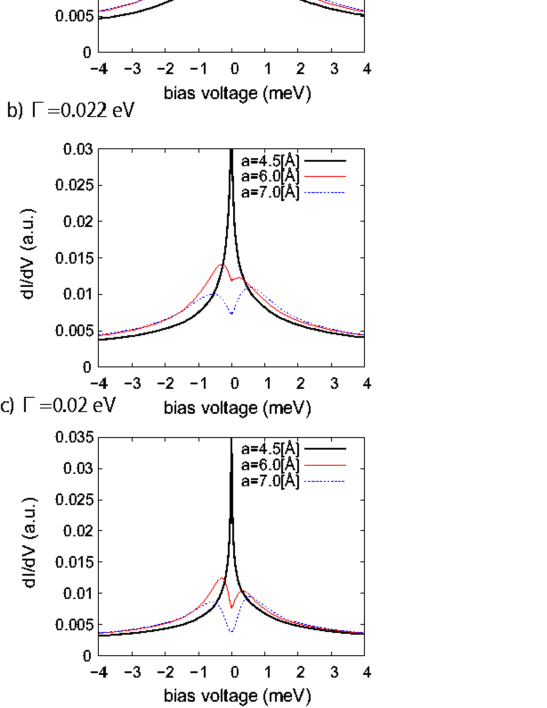
Figure 3: dI/dV calculation results at several adatom separations with a) $\Gamma=0.025$eV ($T_{K}$=6.64K), b)$\Gamma=0.022$eV ($T_{K}$=3.07K), and c) $\Gamma=0.02$eV ($T_{K}$=1.63K). The STM tip is placed at $z_{p}=4.0$Å. We set $R_{S}=3.0$Å  and $W_{0}=T_{0}=0.02$eV.

At $a=5.0$Å  and $a=9.0$Å, there is a sharp peak structure near the Fermi level. With these adatom separations, the RKKY interaction is weak antiferromagnetic and the Kondo effect is dominantMinamitani et al. (2009b). The sharp peak corresponds to the Yosida-Kondo resonance. With our settings, the antiferromagnetic RKKY interaction becomes largest around $a=7.0$Å. As the adatom separation becomes close to 7.0Å, the peak structure changes gradually. When $\Gamma=0.025$eV, the dI/dV spectra broaden as $a$ becomes close to 7.0Å. However, when $\Gamma=0.022$eV, a dip structure appears near the Fermi level. This dip structure develops to a deeper one as $\Gamma$ decreases.

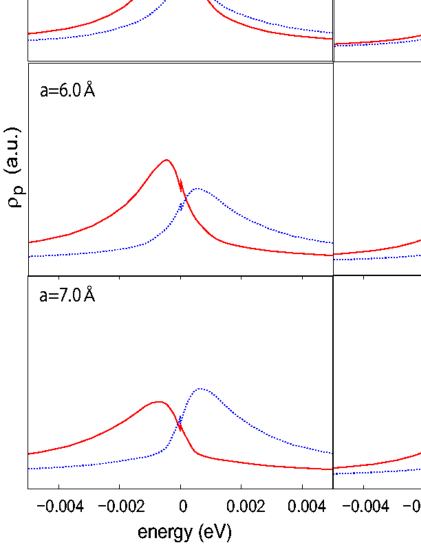
Figure 4: Single electron excitation spectra of adatom electrons for each parity channel.

We find that the “parity splitting” of the single electron excitation spectra is the origin of the dip structure in the dI/dV spectra. As shown in eq.(13), the operators in the model Hamiltonian are indexed by the parity $q$. Thus, the obtained physical properties such as single electron excitation spectra are divided with respect to the parity. The dI/dV spectra are proportional to the average of the single electron excitation spectra of adatom electrons on each parity channel ($\rho_{+}$,$\rho_{-}$). As shown in Fig.4, $\rho_{+}$ and $\rho_{-}$ have different peak positions. The asymmetry of the spectra results from the difference in the coupling between the adatom and conduction band in each parity channel (See eq.(13) and eq.(15)). Previous studies shows that the parity splitting is one of the signatures of the smearing out of the critical point due to the breaking of the e-h symmetry Affleck et al. (1995); Sakai and Shimizu (1992a). In the present study, based on the model Hamiltonian (1), the tunneling matrix element between the localized d-electrons and the metal surface conduction electrons has energy dependence, which breaks the e-h symmetry.

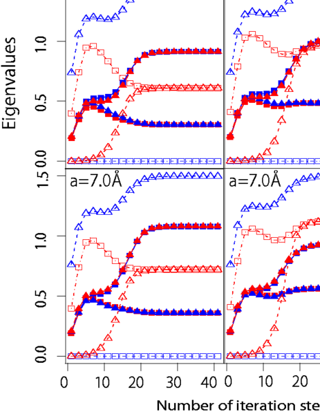
Figure 5: Flows of the low-lying many-particle energy levels in odd iterations. $N+1$ corresponds to the iteration step number. In this calculation we calculate at $a=5.0,6,0,7,0$Åa) $\Gamma=0.025$eV b)$\Gamma~{}0.02$eV. The states are labeled by the quantum numbers total charge $Q$, total spin $S$, and total parity $P$.

In order to investigate the electron state, we plotted the flow of low lying many-particle energies in the NRG calculation with several adatom separations (Fig.5). The states are labeled by the quantum numbers total charge $Q$, total spin $S$, and total parity $P$. Here we show the flows of the lowest state for (Q,2S,P)=(0,0,1),(1,1,1),(-1,1,1),(1,1,-1),(-1,1,-1),(0,2,1) and (0,2,-1). The Q=0,2S=0,P=1 state is the ground state. Q=$\pm 1$,2S=1and P=$\pm 1$ states are the single electron (hole) excited states. When $a=5.0$Å, as $N$ increases, the energy of ($\pm 1$, 1, $\pm 1$) state decreases relatively. This indicates the energy gain from the formation of a singlet between the adatom localized spin and excited state of the conduction electron, i.e., the Yosida-Kondo singlet. However, when $a$ comes close to 7.0Å, the energy of the single particle excited states do not decrease so much but keep considerable value in large N.

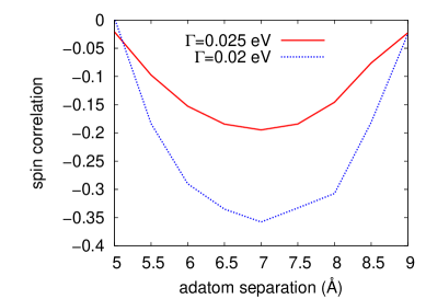
Figure 6: Spin correlation function as a function of adatom separation.

From the calculation result for the spin correlation function between adatom localized spin(Fig.6), we conclude that this large energy of single particle excitation states originates from the interruption of the Yosida-Kondo singlet formation by the strong antiferromagnetic correlation between the localized spins. In our model, the e-h symmetry breaking connect the antiferromagnetic region and the Kondo region continuously and the ground state would be the hybrid of the localized spin-spin singlet state and the Yosida-Kondo singlet state. As the antiferromagnetic correlation between localized spin becomes large, the localized spin-spin singlet state would become dominant and suppress the excitation at the Fermi level, which results in the dip structure of dI/dV. Thus, the dip structure in dI/dV would enable us to detect the strong antiferromagnetic correlation between localized spins.

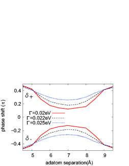
Figure 7: Phase shift as a function of adatom separation. (in units of $\pi$ radians)

We can also discuss about the fixed point Hamiltonian and the phase shift estimated from that. As shown in Fig.5, the energy levels converge to some values for large N. This means that the Hamiltonian becomes close to the fixed point Hamiltonian of renormalization transformationKrishna-murthy et al. (1980a, b); Bulla et al. (2008). In this calculation, we can define the fixed point Hamiltonian as follows;

$$H_{eff}^{N} = \Lambda^{(N-1)/2}\bigl{\{}\sum^{N-1}_{q=\pm,n=0}\eta_{qn}(f^{\dagger}_{qn}f_{qn}+H.C.)$$ (17)

$$+ K_{q}f^{\dagger}_{0}f_{0}\bigr{\}}$$

$q=\pm$ is the parity index. The second term with $K_{q}$ is related to the influence of potential scattering in each channel. The strength of the potential scattering $K_{q}$ and the phase shift $\delta_{q}$ have the following relation:

$$\delta_{q}=-\tan^{-1}(\pi\rho K_{q})$$ (18)

We estimate $K_{q}$ in each conduction channel by comparing the many-particle energy of first excited state in the last iteration of NRG calculation with that of Eq.(17).
  The phase shift is related to the number of electrons and holes which are virtually bounded by localized spin – i.e., the phase shift is a barometer of the existence of the Kondo effect. If $\delta_{\pm}=\pi/2$, it means that one electron-hole pair is bounded to each localized spin and quenches it individually (i.e,. two Yosida-Kondo singlets are formed). On the other hand, $\delta_{\pm}=0$ indicates that a localized spin-spin singlet is formed Sakai and Shimizu (1992a). In Fig.7, we show the result of the phase shift calculation as a function of adatom separation with several values of $\Gamma$.
  The phase shift changes gradually and has an intermediate value between $\pm\pi/2$ to 0 (Fig. 7). The smallest value of $\delta_{\pm}$ becomes close to 0 as $\Gamma$ decreases. This result also indicates that the dip structure around $a=7.0$Å  originates from the dominance of the spin-spin singlet state in the ground state. Though the values of $\delta_{\pm}$ at each adatom separation are different by $\Gamma$, the change of $\delta_{\pm}$ is smooth in all cases. If a critical point separates the Kondo region and the antiferromagnetic region, the possible values of $\delta_{\pm}$ are only 0 or $\pm\pi/2$ Sakai and Shimizu (1992a, b); Silva et al. (1996) . The intermediate value of $\delta_{\pm}$ would result from the crossover transition and supports the conclusion that there is no critical point in the system of a magnetic dimer on a metal surface.

IV Summary

To investigate how the transition between the Kondo effect dominant region and the antiferromagnetic RKKY interaction dominant region can be observed through scanning tunneling spectroscopy (STS), we calculate the differential conductance (dI/dV) corresponding to STS measurements for two magnetic atoms adsorbed on a metal surface with the aid of the numerical renormalization group technique. We find that the peak structure of the dI/dV spectra changes gradually as a function of the adatom separation and the coupling ($\Gamma$) between the adatoms and the metal surface conduction band. When $\Gamma$ becomes small, the peak disappears and a dip structure appears near the Fermi level. This dip structure originates from the parity splitting of the single electron excitation spectra and the manifestation of the strong antiferromagnetic correlation between the localized spins. The result of the phase shift calculation supports the conclusion that there is no critical point between the Kondo effect dominant region and the antiferromagnetic RKKY interaction dominant region but a crossover transition connect these regions.
  In conclusion, we show that the crossover transition from the Kondo region to the antiferromagnetic region in two-impurity Kondo effect can be observed through the change of the STS spectra. In particular, the existence of the strong antiferromagnetic correlation between localized spins are observed as dip structures in the dI/dV. Our results indicate the possibility in STM observation with the resolution of magnetic interactions on surface system, which would contribute to the realization of spintronics.

V Acknowledgments

This work is supported by the Ministry of Education, Culture, Sports, Science and Technology of Japan (MEXT) through their Special Coordination Funds for the Global Center of Excellence (GCOE) program (H08) “Center of Excellence for Atomically Controlled Fabrication Technology”, Grant-in-Aid for Scientific Research (C)(19510108); and the New Energy and Industrial Technology Development Organization (NEDO). E. Minamitani would like to thank the NIHON L’OREAL K.K. and Japan Society for the Promotion of Science (JSPS) for financial support and H. Matsuura (Osaka Univ.) for helpful discussions. Some of the calculations presented here were performed using the computer facilities of Cyber Media Center (Osaka University), the Institute of Solid State Physics (ISSP Super Computer Center, University of Tokyo), and the Yukawa Institute (Kyoto University).

References

- Jayaprakash et al. (1981) C. Jayaprakash, H. R. Krishna-murthy, and J. W. Wilkins, Phys. Rev. Lett. 47, 737 (1981).
- Jones et al. (1988) B. A. Jones, C. M. Varma, and J. W. Wilkins, Phys. Rev. Lett. 61, 125 (1988).
- Jones and Varma (1989) B. A. Jones and C. M. Varma, Phys. Rev. B 40, 324 (1989).
- Affleck et al. (1995) I. Affleck, A. W. W. Ludwig, and B. A. Jones, Phys. Rev. B 52, 9528 (1995).
- Sakai and Shimizu (1992a) O. Sakai and Y. Shimizu, J. Phys. Soc. Jpn 61, 2333 (1992a).
- Silva et al. (1996) J. B. Silva, W. L. C. Lima, W. C. Oliveira, J. L. N. Mello, L. N. Oliveira, and J. W. Wilkins, Phys. Rev. Lett. 76, 275 (1996).
- Kasai et al. (2000) H. Kasai, W. A. Dio, and A. Okiji, J. Elec. Spec. Rel. Phenom. 109, 63 (2000).
- Kawasaka et al. (1999) T. Kawasaka, H. Kasai, W. A. Dio, and A. Okiji, J. Appl. Phys. 86, 6970 (1999).
- Shimada et al. (2003) Y. Shimada, H. Kasai, H. Nakanishi, W. A. Dio, A. Okiji, and Y. Hasegawa, J. Appl. Phys. 94, 334 (2003).
- Crommie et al. (1993) M. F. Crommie, C. P. Lutz, and D. M. Eigler, Science 262, 218 (1993).
- Heinrich et al. (2004) A. J. Heinrich, J. A. Gupta, C. P. Lutz, and D. M. Eigler, Science 306, 466 (2004).
- Dio et al. (2006) W. A. Dio, H. Kasai, E. T. Rodulfo, and M. Nishi, Thin Solid Films 509, 168 (2006).
- Madhavan et al. (1998) V. Madhavan, W. Chen, T. Jamneala, M. F. Crommie, and N. S. Wingreen, Science 280, 567 (1998).
- Minamitani et al. (2009a) E. Minamitani, H. Nakanishi, W. A. Dio, and H.Kasai, J. Phys. Soc. Jpn. 78, 084705 (2009a).
- Minamitani et al. (2009b) E. Minamitani, H. Nakanishi, W. A. Dio, and H.Kasai, Solid State Commun. 149, 1241 (2009b).
- Merino et al. (2009b) J. Merino, L. Borda, and P. Simon, Europhys. Lett. 85, 47002 (2009b).
- Wahl et al. (2007) P. Wahl, P. Simon, L. Diekhöner, V. S. Stepanyuk, P. Bruno, M. A. Schneider, and K. Kern, Phys. Rev. Lett. 98, 056601 (2007).
- Otte et al. (2008) A. F. Otte, M. Ternes, K. V. Bergmann, S. Loth, H. Brune, C. P. Lutz, C. F. Hirjibehedin, and A. J. Heinrich, Nature Physics 4, 847 (2008).
- Rammer and Smith (1986) J. Rammer and H. Smith, Rev. Mod. Phys. 58, 323 (1986).
- Krishna-murthy et al. (1980a) H. R. Krishna-murthy, J. W. Wilkins, and K. G. Wilson, Phys. Rev. B 21, 1044 (1980a).
- Krishna-murthy et al. (1980b) H. R. Krishna-murthy, J. W. Wilkins, and K. G. Wilson, Phys. Rev. B 21, 1003 (1980b).
- Campo et al. (2005) V. L. Campo, Jr., and L. N. Oliveira, Phys. Rev. B 72, 104432 (2005).
- Bulla et al. (2008) R. Bulla, T. A. Costi, and T. Pruschke, Rev. Mod. Phys. 80, 395 (2008).
- Yoshimori and Kasai (1986) A. Yoshimori and H. Kasai, Solid State Commun. 58, 259 (1986).
- Sakai and Shimizu (1992b) O. Sakai and Y. Shimizu, J. Phys. Soc. Jpn 61, 2348 (1992b).