Adiabatic quantum computation along quasienergies

Abstract

The parametric deformations of quasienergies and eigenvectors of unitary operators are applied to the design of quantum adiabatic algorithms. The conventional, standard adiabatic quantum computation proceeds along eigenenergies of parameter-dependent Hamiltonians. By contrast, discrete adiabatic computation utilizes adiabatic passage along the quasienergies of parameter-dependent unitary operators. For example, such computation can be realized by a concatenation of parameterized quantum circuits, with an adiabatic though inevitably discrete change of the parameter. A design principle of adiabatic passage along quasienergy is recently proposed: Cheon’s quasienergy and eigenspace anholonomies on unitary operators is available to realize anholonomic adiabatic algorithms [Tanaka and Miyamoto, Phys. Rev. Lett. 98, 160407 (2007)], which compose a nontrivial family of discrete adiabatic algorithms. It is straightforward to port a standard adiabatic algorithm to an anholonomic adiabatic one, except an introduction of a parameter $|{}v{}\rangle$, which is available to adjust the gaps of the quasienergies to control the running time steps. In Grover’s database search problem, the costs to prepare $|{}v{}\rangle$ for the qualitatively different, i.e., power or exponential, running time steps are shown to be qualitatively different. Curiously, in establishing the equivalence between the standard quantum computation based on the circuit model and the anholonomic adiabatic quantum computation model, it is shown that the cost for $|{}v{}\rangle$ to enlarge the gaps of the eigenvalue is qualitatively negligible.

I Introduction

An adiabatic passage along an eigenenergy of a Hamiltonian with slowly-varying parameter Messiah (1999) provides one of the simplest ways to control quantum states. Recently, one of largest-scale applications of the adiabatic passage to compose an algorithm for classically intractable problems is proposed by Farhi et al. Farhi et al. (2000). Their adiabatic passage connects a quantum state, which is supposed to be easy to prepare, to a state that represents a solution of, for example, a satisfiability problem. Farhi et al. showed a systematic way to design a parameter-dependent Hamiltonian with local interactions of qubits only which governs the adiabatic passage. We will call this approach the standard adiabatic quantum computation (SAQC) as we later introduce a new approach to be distinguished from the SAQC. Recently, the standard adiabatic quantum computation is proven to have the same computational power as the standard quantum computation in terms of the computational complexity Aharonov et al. (2007). It is still an open question whether the adiabatic approach really solve the classically intractable problems efficiently as we can see the promising numerical results Farhi et al. (2001); Schützhold and Schaller (2006) as well as the reports of disastrous slowdown Žnidarič (2005); Žnidarič and Horvat (2005); Farhi et al. (2008).

In many studies of SAQC, e.g., in the simulations of SAQC by quantum circuits Farhi et al. (2000) and classical digital computers Hogg (2003), or in experimental realizations where the adiabatic changes of coupling constants are infeasible Steffen et al. (2003); not (a), it is inevitable to introduce the discretization of the adiabatic deformation of parameters. In such cases, the time evolution in the computational process is realized by the products of parameterized unitary operators, each of which represents a computational step to emulate the time evolution for the unit of time. Due to the tolerance of the adiabatic passage against small perturbations, the discretization of the time evolution, in general, provides a good approximation of SAQC. The discretization process however can be considered to introduce an alternative model of adiabatic quantum computation. The state vector follows the adiabatic change of an eigenvector of a unitary operator, where the definition of eigenenergy can be inapplicable even in any approximate sense. This scheme, which we call discrete adiabatic quantum computation (DAQC), will be formulated based on the adiabatic passage along a quasienergy Zel’dovich (1967), or equivalently, an eigenangle of slowly-varying unitary operator.

DAQC is useful to generalize quantum adiabatic algorithm, which we will show in this paper. A family of DAQC that essentially relies on the adiabatic passage along a quasienergy is recently proposed by one of the authors Tanaka and Miyamoto (2007). Here the adiabatic passage is composed with a help of Cheon’s eigenvalue anholonomy Cheon (1998); Tanaka and Miyamoto (2007); Miyamoto and Tanaka (2007); Cheon and Tanaka (2009), which enables us to design adiabatic passages that visit all eigenstates of a given unperturbed Hamiltonian. This adiabatic scheme, which will be called anholonomic adiabatic quantum computation (AAQC), composes an interesting and nontrivial family of DAQC. In particular, AAQC does not approximate SAQC, and hence the question whether AAQC is equivalent to the standard quantum computation naturally arises Tanaka and Miyamoto (2007).

In this paper, we establish a formulation of AAQC and elucidate its equivalence to the standard quantum computation. To achieve this, we start from the formulation of DAQC, the most general family of the adiabatic algorithm, in Section II. It turns out that AAQC, which composes a subset of DAQC, offers us a systematic way to design nontrivial instances of DAQC (Section III). We show how the performance of AAQC can be evaluated in the Grover’s unstructured database search problem Grover (1997). It is shown that an ingredient of AAQC strongly affects the performance that is determined by the “gap” of eigenvalues (Section IV). In Section V, we show that the anholonomic adiabatic quantum computation model is equivalent with the standard quantum computation, through a modification of Aharonov et al.’s proof Aharonov et al. (2007) of the equivalence between the standard quantum computation and the standard adiabatic computation model. There, it turns out that the control of the gap in AAQC discussed in Section IV plays crucial role to show the equivalence.

II Discrete Adiabatic Quantum Computation

In this section, we will introduce discrete adiabatic quantum computation (DAQC) in order to facilitate our study of AAQC in the following sections. First, a formulation of DAQC, which offers a unified framework for the adiabatic algorithm, is established in Section II.1. Second, it is shown that a family of DAQC approximates SAQC in Section II.2. Third, we show the equivalence of DAQC and the standard quantum computation in Section II.3.

II.1 Formulation of DAQC

We will design a computational system that involves $n$ qubits. This naturally introduces the concept of locality among qubits in the computational system. Namely, if an operation involves only few, $n$-independent numbers of qubits, the operation is called local. The time evolution of the quantum state is governed by a unitary operator $\hat{U}_{s}$ with an “adiabatic” parameter $s$. In the stroboscopic description of the time evolution, a unit step evolution of a quantum state from $|{}\psi^{\prime}{}\rangle$ to $|{}\psi^{\prime\prime}{}\rangle$ is described by a quantum map Berry et al. (1979)

$$|{}\psi^{\prime\prime}{}\rangle=\hat{U}_{s}|{}\psi^{\prime}{}\rangle.$$ (1)

Since the quantum map is iterated extensively to realize an adiabatic passage, $\hat{U}_{s}$ is required to be efficiently implementable, whose definition will be introduced so as to be compatible with the one for quantum circuits. First, we explain a construction of $\hat{U}_{s}$ from a product of local unitary operations. The unitary operator $\hat{U}_{s}$ accordingly has a natural counterpart of a quantum circuit, where each factor of $\hat{U}_{s}$ corresponds to an element of the circuit. If the number of the factors is bounded asymptotically by a polynomial of $n$, $\hat{U}_{s}$ is called to be efficiently implementable. The number of the iterations of the quantum map characterizes the computational complexity of the algorithm.

Next we discuss the case that $\hat{U}_{s}$ is realized by a time evolution induced by a time-dependent Hamiltonian $\hat{H}_{s}(t)$ during a finite time interval (say, $0\leq t\leq T$), i.e.,

$$\hat{U}_{s}=\mathop{\rm exp}_{\leftarrow}\left(-\frac{i}{\hbar}\int_{0}^{T}\hat{H}_{s}(t)dt\right),$$ (2)

where $\mathop{\rm exp}_{\leftarrow}$ denotes the time-orderd exponential. We restrict ourselves to the case that $\hat{H}_{s}(t)$ is composed by a finite number of local interaction terms. In particular, we call $\hat{H}_{s}(t)$ efficiently implementable, when the number of the local interaction terms for $\hat{H}_{s}(t)$ is bounded by a polynomial of $n$. Based on the argument by Lloyd Lloyd (1996); Farhi et al. (2000), the efficiency discussed here is equivalent to the efficiency for quantum circuits mentioned above. In addition to the two approaches of the implementation of $\hat{U}_{s}$, it is possible to merge two approaches to construct $\hat{U}_{s}$. An example will be shown in Section V.

To introduce an adiabatic passage for a quantum map, the eigenvalue problem of $\hat{U}_{s}$ is explained more precisely. An eigenvalue of $\hat{U}_{s}$ is a unimodular complex number, due to the unitarity. We parameterize the eigenvalue $e^{-i\theta(s)}$ by a real number $\theta(s)$, which is called an eigenangle not (b). By definition, the space of eigenangle has a period of $2\pi$. Since we assumed in the following that a unit time interval $T$ is associated with the quantum map $\hat{U}_{s}$, e.g. $\hat{U}_{s}$ is induced by a Hamiltonian time evolution during time interval $T$, an eigenangle $\theta(s)$ provides a characteristic energy scale $E(s)\equiv\theta(s)\hbar T^{-1}$, which is called quasienergy Zel’dovich (1967) and determined up to modulo $2\pi\hbar{}T^{-1}$. Corresponding to $E(s)$, let $|{}\xi(s){}\rangle$ be an eigenvector of $\hat{U}_{s}$, i.e., they satisfy the eigenvalue equation $\hat{U}_{s}|{}\xi(s){}\rangle=e^{-iTE(s)/\hbar}|{}\xi(s){}\rangle$. We further require that $E(s)$ and $|{}\xi(s){}\rangle$ are smooth with respect to $s$. The eigenvector $|{}\xi(s){}\rangle$ is also called a stationary state, due to its characteristic in dynamics. For the fixed value of $s$, the state $|{}\xi(s){}\rangle$ is invariant under the time evolution induced by successive application of $\hat{U}_{s}$ up to the accumulated dynamical phase.

To explain a discrete adiabatic behavior of the state vector, let us change the value of $s$ from $0$ to $s_{\rm max}$, under a successive application of $\hat{U}_{s}$ during $L$ ($\gg 1$) steps. Let $s_{l}$ be the value of $s$ at $l$-th step, where $s_{0}=0$ and $s_{L}=s_{\rm max}$. The exact final state is

$$|{}\Psi_{L}{}\rangle\equiv\hat{U}_{s_{L}}\hat{U}_{s_{L-1}}\ldots\hat{U}_{s_{1}}|{}\xi(0){}\rangle.$$ (3)

The adiabatic theorem for quantum maps Hogg (2003) ensures that $|{}\Psi_{L}{}\rangle$ converges to $|{}\xi(s_{\rm max}){}\rangle$ up to the global phase as $L\to\infty$, if the gaps between the nearest eigenangles are large enough. In reality, $L$ is always kept to be finite and the adiabatic time evolution is consequently not exact. A criterion to determine $L$ is the condition that the time evolution obeys the adiabatic time evolution within an error $\epsilon$, i.e., $\bm{\|}|{}\Psi_{L}{}\rangle\langle{}\Psi_{L}{}|-|{}\xi(s_{\rm max}){}\rangle\langle{}\xi(s_{\rm max}){}|\bm{\|}<\epsilon$. This is equivalent with $L\geq L(\epsilon)$, where $L(\epsilon)$ is an appropriate lower bound. Here, the most important source of the error in the asymptotic regime $L\to\infty$ is nonadiabatic transition Nakamura (2002). Hence the crudest estimate of $L(\epsilon)$ will be determined by the Landau-Zener-Stückelberg formula with a modification that comes from the use of quasienergies Breuer and Holthaus (1989), instead of eigenenergy, for the discrete adiabatic processes.

To summarize the above argument, a definition of discrete adiabatic computation (DAQC) is given: An instance of DAQC is specified by an efficiently implementable unitary operator $\hat{U}_{s}$, an initial state $|{}\Psi_{0}{}\rangle$, and a schedule $\left\{s_{l}\right\}_{l=0}^{L}$ of the adiabatic parameter from $s_{0}=0$ to $s_{L}=s_{\rm max}$ with the number of steps $L$. DAQC is designed to transport the initial state vector $|{}\Psi_{0}{}\rangle$, which is the eigenstate $|{}\xi(s=0){}\rangle$ of $\hat{U}_{0}$, to the target state $|{}\xi(s=s_{max}){}\rangle$ within an error $\epsilon$ through the continuous deformation of an eigenstate $|{}\xi(s){}\rangle$ of $\hat{U}_{s}$. The initial state is be prepared from $|{}0{}\rangle$ by an efficiently implementable unitary operator $\hat{U}_{\rm I}$, i.e. $|{}\Psi_{0}{}\rangle=\hat{U}_{\rm I}|{}0{}\rangle$. We need to make $L$ large enough so that the final state $|{}\Psi_{L}{}\rangle=\hat{U}_{s_{L}}\hat{U}_{s_{L-1}}\ldots\hat{U}_{s_{1}}|{}\Psi_{0}{}\rangle$ of the computation is a good approximation of the target state of the computation $|{}\xi(s_{\rm max}){}\rangle$. The running time $L(\epsilon)$ is the minimum value of $L$ to achieve that the distance between the final state $|{}\Psi_{L}{}\rangle$ and $|{}\xi(s_{\rm max}){}\rangle$ is smaller than a given error $\epsilon$.

II.2 DAQC from SAQC through the discretization of continuous-time evolution

As a way to construct DAQC, the discretizations of standard adiabatic quantum computation (SAQC) are explained for a pedagogic purpose. As mentioned in the introduction, many studies of SAQC are done through the discretization of the variation of the adiabatic parameter. The discretized time evolution is introduced so that it approximates well the ideal, continuous-time evolution. We first explain the standard adiabatic quantum computation. A computational system is specified by a Hamiltonian $\hat{H}(s)$, which can be decomposed into a finite number of local Hamiltonians, with an adiabatic parameter $s$. We assume, without loss of generality, that the initial and the final values of $s$ are $0$ and $s_{\text{max}}$, respectively. The initial state $|{}\Psi_{0}{}\rangle$ must be the ground state of $\hat{H}_{\rm B}\equiv\hat{H}(0)$, which can be efficiently prepared. The target of the computation is the ground state of $\hat{H}_{\rm P}\equiv\hat{H}(s_{\text{max}})$. For a given time-dependence of $s(t)$ with $0\leq t\leq T_{\text{max}}$, $s(0)=0$, and $s(T_{\text{max}})=s_{\text{max}}$, the exact final state of the computation (of the unitary evolution part) is

$$\mathop{\rm exp}_{\leftarrow}\left(-i\int_{0}^{T_{\text{max}}}\hat{H}\bm{(}s(t)\bm{)}dt\right)|{}\Psi_{0}{}\rangle.$$ (4)

In the adiabatic limit $T_{\text{max}}\to\infty$, the finial state converges to the target for the final state. The running time of the computation is the minimum value of $T_{\text{max}}$ that keeps the distance between the finial and the target states within a given error $\epsilon$.

A discretization of the time-dependence in $s(t)$ gives us an instance of DAQC. For a discretization of time $t_{l}$ ($0\leq l\leq L$), we introduce a piecewise constant function $\tilde{s}(t)=s_{l}\equiv\left[s(t_{l-1})+s(t_{l})\right]/2$ for $t_{t-1}<t<t_{l}$. For the sake of simplicity, we set $s_{0}\equiv 0$ and $t_{-1}\equiv-t_{1}$. Accordingly, we have a unitary operator of a time interval $(t_{l-1},t_{l})$:

$$\hat{U}_{l}\equiv\exp\left[-i\hat{H}(s_{l})(t_{l}-t_{l-1})\right].$$ (5)

The final state of a SAQC with the schedule $\tilde{s}(t)$ is

$$\hat{U}_{L}\hat{U}_{L-1}\ldots\hat{U}_{1}|{}\Psi_{0}{}\rangle.$$ (6)

Namely, we obtain a DAQC from a SAQC, since $|{}\Psi_{0}{}\rangle$ is also an eigenvector of $\hat{U}_{0}=e^{-i\hat{H}(0)(t_{0}-t_{-1})}$. We may expect the convergence of a DAQC to the original SAQC in the limit $L\to\infty$. For finite $L$, the DAQC is an approximation of the SAQC. Hence we may regard that the DAQC approximately follows the adiabatic passage built on the parametrically varying eigenenergy.

II.3 DAQC is equivalent to the standard quantum computation

Now we examine the equivalence of DAQC and the standard quantum computation, in the sense of computational complexity. First, it is straightforward to see that a DAQC is efficiently simulated by a quantum circuit from the definition above. Second, for the inverse argument, i.e., whether a quantum circuit can be simulated by a DAQC, we need to remind that DAQC involves a rather wide class of computation. In particular, as is explained above, DAQC contains the discretizations of the standard adiabatic quantum computation, which are proven to be equivalent with the standard quantum computation Aharonov et al. (2007). Hence, it is trivial to conclude that DAQC are equivalent with the standard quantum computation.

Much more serious question on the equivalence arises when we examine a subclass of DAQC, by introducing an alternative design of DAQC, where the adiabatic passage built on the parametrically varying eigenenergy is inapplicable. Instead, an adiabatic passage built on a quasienergy needs to be employed. We will discuss such an example in the next section.

III Anholonomic adiabatic quantum computation

In this section, anholonomic adiabatic quantum computation (AAQC), which compose a subclass of DAQC, is introduced. The adiabatic passages of AAQC can be constructed with the help of Cheon’s eigenvalue and eigenspace anholonomies, which will be explained in Section III.1. Subsequently, a formulation of AAQC is introduced in Section III.2. Finally, the simulation of AAQC by quantum circuits is examined in Section III.3, where a crucial ingredient to determine the cost of the simulation is identified.

III.1 Cheon’s anholonomies for unitary operators

First of all, we explain Cheon’s eigenvalue and eigenspace anholonomies Cheon (1998) and their realization in a periodically pulsed system under a rank-$1$ perturbation Tanaka and Miyamoto (2007). This offers a systematic design principle for adiabatic passages, in particular, adiabatic quantum computation, along parametric changes of unitary operators Miyamoto and Tanaka (2007). We assume that the spectrum of an “unperturbed” Hamiltonian $\hat{H}_{0}$ is discrete, finite and non-degenerate. We will examine a periodically-pulsed driven system described by the following “kicked” Hamiltonian:

$$\hat{H}_{s}(t)\equiv\hat{H}_{0}+s|{}v{}\rangle\langle{}v{}|\sum_{n\in\mathbb{Z}}\delta(t-nT),$$ (7)

where $T$ and $s$ are the period and the strength of the perturbation, and $|{}v{}\rangle$ is assumed to be normalized. The kicked Hamiltonian (7) naturally induces a quantum map $|{}\psi_{n+1}{}\rangle=\hat{U}_{s}|{}\psi_{n}{}\rangle$, where $|{}\psi_{n}{}\rangle$ is the state vector just before the kick at $t=nT$ and

$$\hat{U}_{s}\equiv e^{-i\hat{H}_{0}T}e^{-is|{}v{}\rangle\langle{}v{}|}$$ (8)

is the corresponding Floquet operator. We set $\hbar=1$ in the following.

We remark the topological structure of the parameter space $s$ for the Floquet operator $\hat{U}_{s}$ (8). From $e^{-is|{}v{}\rangle\langle{}v{}|}=(1-|{}v{}\rangle\langle{}v{}|)+e^{-is}|{}v{}\rangle\langle{}v{}|$ , both $\hat{U}_{s}$ and its spectrum is periodic in $s$ with period $2\pi$. Hence we may identify the parameter space of $s$ as a circle.

We explain what will happen for each quasienergy and each eigenvector of $\hat{U}_{s}$ (8) when we increase $s$ for a period. Let us consider the ground energy $E^{\prime}$ and the first excited eigenenergy $E^{\prime\prime}$ of $\hat{H}_{0}$ ($E^{\prime}<E^{\prime\prime}$) not (c). The corresponding normalized eigenvectors are denoted by $|{}E^{\prime}{}\rangle$ and $|{}E^{\prime\prime}{}\rangle$, respectively. For simplicity, we employ a normalized vector $|{}v{}\rangle=a|{}E^{\prime}{}\rangle+b|{}E^{\prime\prime}{}\rangle$, where $a\neq 0$, $b\neq 0$ and $|a|^{2}+|b|^{2}=1$, so that the subspace spanned by $|{}E^{\prime}{}\rangle$ and $|{}E^{\prime\prime}{}\rangle$ is invariant under $\hat{U}_{s}$. Accordingly, in the subspace, which we will focus on, $\hat{U}_{s}$ is a $2$-dimensional matrix effectively. Let $|{}\xi_{0}(s){}\rangle$ be the eigenvector of $\hat{U}_{s}$ with $|{}\xi_{0}(0){}\rangle=|{}E^{\prime}{}\rangle$ and $E_{0}(s)$ the corresponding quasienergy, whose branch is chosen as $[E^{\prime},E^{\prime}+2\pi T^{-1})$, i.e., $E^{\prime}<E^{\prime\prime}<E+2\pi T^{-1}$. Since $\partial_{s}E_{0}(s)=T^{-1}\langle{}\xi_{0}(s){}|{}v{}\rangle\langle{}v{}|{}\xi_{0}(s){}\rangle$ is positive, $E_{0}(s)$ increases as $s$ increases. At the same time, because of the periodicity of $\hat{U}_{2\pi}=\hat{U}_{0}$, $E_{0}(2\pi)=E^{\prime}+\int_{0}^{2\pi}\left[\partial_{s}E_{0}(s)\right]ds$ must be equal to $E^{\prime}$ or $E^{\prime\prime}$ (modulus $2\pi T^{-1}$). The above choice of $|{}v{}\rangle$ ensures $0<\partial_{s}E_{0}(s)<2\pi T^{-1}$, i.e., $E^{\prime}<E_{0}(2\pi)<E^{\prime}+2\pi T^{-1}$. Hence we have $E_{0}(2\pi)=E^{\prime\prime}$, which implies a presence of quasienergy anholonomy. The corresponding eigenvector $|{}\xi_{0}(s){}\rangle$ arrives at $|{}E^{\prime\prime}{}\rangle$ at $s=2\pi$. Thus the minimum example of a path along quasienergy anholonomy $E_{0}(s)$ is shown. Along the path, an adiabatic increment of $s$ for a period of its parameter space (i.e., from $0$ to $2\pi$) transfers the state vector that is initially prepared to be $|{}E^{\prime}{}\rangle$, to $|{}E^{\prime\prime}{}\rangle$.

So far, we did not specify $|{}v{}\rangle$, except that it is a superposed state of $|{}E^{\prime}{}\rangle$ and $|{}E^{\prime\prime}{}\rangle$, because the quasienergy anholonomy do not depend on the details of $|{}v{}\rangle$. For example, the quasienergy anholonomy persists even under adiabatically slow fluctuations of $|{}v{}\rangle$. On the other hand, $|{}v{}\rangle$ affects on the precise shape of $E_{0}(s)$ and adjacent quasienergy curves. Namely, $|{}v{}\rangle$ determines the quasienergy gaps between neighboring levels of $E_{0}(s)$ and accordingly a timescale for adiabatic passages.

Extensions of the quasienergy anholonomy for multilevels are straightforward Tanaka and Miyamoto (2007); Miyamoto and Tanaka (2007). For example, if we choose $|{}v{}\rangle$ that has non-zero overlapping with all eigenvectors of $\hat{H}_{0}$, $E_{0}(2\pi n)$ is the $n$-th excited energy of $\hat{H}_{0}$ not (d). Thus $E_{0}(s)$ connects all the eigenvalues of $\hat{H}_{0}$ to offer a path for adiabatic passages with adiabatic increments of $s$.

III.2 Formulation of AAQC

An anholonomic adiabatic quantum algorithm can be described based on the standard adiabatic algorithm. The standard adiabatic algorithm is specified by a parameter-dependent Hamiltonian $H(s)$ on the Hilbert space $\mathcal{H}_{\rm A}$. Here, we employ the simplest case that $H(s)$ is linear in $s$: $\hat{H}(s)=(1-s)\hat{H}_{\rm B}+s\hat{H}_{\rm P}$, where $\hat{H}_{\rm B}$ and $\hat{H}_{\rm P}$ are the initial and the final Hamiltonians, respectively. We impose that $\hat{H}_{\rm B}$ has non-degenerate ground state $|{}0_{\rm B}{}\rangle$ with the ground energy $0$. The finial Hamiltonian $\hat{H}_{\rm P}$ is a cost function of the problem to solve. Namely, an eigenvalue of $\hat{H}_{\rm P}$ indicates a “distance” between the corresponding eigenvector and the answer of the problem. We assume that the answer is unique and let $|{}x{}\rangle$ be the ground state of $\hat{H}_{\rm P}$. To reuse $\hat{H}_{\rm B}$ and $\hat{H}_{\rm P}$ in the anholonomic approach, the maximum eigenvalues of $\hat{H}_{\rm B}$ and $\hat{H}_{\rm P}$ need to be finite.

We now explain an implementation of an anholonomic adiabatic quantum processor under the assumption that the standard adiabatic quantum processor is available. The state space $\mathcal{H}_{\rm A}$, and its Hamiltonians $\hat{H}_{\rm B}$ and $\hat{H}_{\rm P}$ are reused. An additional qubit is employed as a “control register,” whose Hilbert space $\mathcal{H}_{\rm C}$ has a complete orthonormal system $\left\{|{}0{}\rangle,|{}1{}\rangle\right\}$. Hence the whole Hilbert space is $\mathcal{H}_{\rm A}\otimes\mathcal{H}_{\rm C}$. Corresponding to the “initial” and “final” states of computation, we introduce two projectors ${\hat{\mathcal{Z}}}^{({\rm c})}\equiv|{}0{}\rangle\langle{}0{}|$ and ${\hat{\mathcal{I}}}^{({\rm c})}\equiv|{}1{}\rangle\langle{}1{}|$, respectively, on $\mathcal{H}_{\rm C}$. Combining these parts, we obtain an unperturbed Hamiltonian

$$\hat{H}_{0}\equiv\hat{H}_{\rm B}\otimes{\hat{\mathcal{Z}}}^{({\rm c})}+(E_{\rm P}+\hat{H}_{\rm P})\otimes{\hat{\mathcal{I}}}^{({\rm c})},$$ (9)

where we assume that $E_{\rm P}$ is positive and smaller than the first excited energy of $\hat{H}_{\rm B}$. It is straightforward to see that the ground energy $0$ and the first excited energy $E_{\rm P}$ of $\hat{H}_{0}$ are nondegenerate. By construction, the ground and the first excited states of $\hat{H}_{0}$ are $|{}-{}\rangle\equiv|{}0_{\rm B}{}\rangle\otimes|{}0{}\rangle$ and $|{}+{}\rangle\equiv|{}x{}\rangle\otimes|{}1{}\rangle$, respectively. We employ the quantum map (8) to realize the quasienergy anholonomy that connects between the ground energy $0$ and the first excited energy $E_{\rm P}$ of $\hat{H}_{0}$ (9). We impose the conditions $\langle{}\pm{}|{}v{}\rangle\neq 0$ for $|{}v{}\rangle$ so that the quasienergy $E_{0}(s)$ of $\hat{U}_{s}$ with $E_{0}(0)=0$ reaches $E_{\rm P}$ at $s=2\pi$. The adiabatic passage along $E_{0}(s)$ ($0\leq{}s\leq 2\pi$) transfers the state vector from $|{}-{}\rangle$ to $|{}+{}\rangle$, then the final state provides the answer. To evaluate the performance of the anholonomic adiabatic quantum computation, we need to obtain the quasienergy gap with respect to the path $E_{0}(s)$. The quasienergy gap depends on the choice of $|{}v{}\rangle$. We will evaluate the gaps for two choices of $|{}v{}\rangle$ in the following sections.

III.3 Costs for simulations of AAQC by quantum circuits

We show how the unitary operator $\hat{U}_{s}$ (8) of the anholonomic adiabatic quantum processor is composed by local quantum circuits, in a similar way explained in Farhi et al. Farhi et al. (2000). From the definition of $\hat{H}_{0}$ (9), $\hat{U}_{s}$ is expressed by a product $\hat{U}_{s}=\hat{U}_{0{\rm B}}\;\hat{U}_{0{\rm P}}\;e^{-is|{}v{}\rangle\langle{}v{}|}$, where $\hat{U}_{0{\rm B}}\equiv e^{-i\hat{H}_{\rm B}\otimes{\hat{\mathcal{Z}}}^{({\rm c})}T}$ and $\hat{U}_{0{\rm P}}\equiv e^{-i(\hat{H}_{\rm P}+E_{\rm P})\otimes{\hat{\mathcal{I}}}^{({\rm c})}T}$.

In the analysis of $\hat{U}_{0{\rm B}}$, we assume that $\hat{H}_{\rm B}$ is composed by $\hat{H}_{{\rm B},j}$, initial Hamiltonians for $j$-th qubit. For example, it is often the case that $\hat{H}_{{\rm B},j}$ is an Hadamard operation. This allows further decomposition:

$$\hat{U}_{0{\rm B}}=e^{-i\hat{H}_{{\rm B},0}\otimes{\hat{\mathcal{Z}}}^{({\rm c})}T}e^{-i\hat{H}_{{\rm B},1}\otimes{\hat{\mathcal{Z}}}^{({\rm c})}T}\cdots e^{-i\hat{H}_{{\rm B},{n-1}}\otimes{\hat{\mathcal{Z}}}^{({\rm c})}T},$$ (10)

where $e^{-i\hat{H}_{{\rm B},j}\otimes{\hat{\mathcal{Z}}}^{({\rm c})}T}=(1-{\hat{\mathcal{Z}}}^{({\rm c})})+{\hat{\mathcal{Z}}}^{({\rm c})}e^{-i\hat{H}_{{\rm B},j}T}$ is a controlled-$1$ bit unitary operation. Hence $\hat{U}_{0{\rm B}}$ is simulated by $n$ controlled-$1$ bit unitary gates.

To examine $\hat{U}_{0{\rm P}}$, assume that $\hat{H}_{\rm P}$ is a cost Hamiltonian of a satisfiability problem, which is composed by clauses $C_{j}$. Let $m$ be the number of the clauses and $\hat{H}_{{\rm P},j}$ a corresponding local Hamiltonian for $C_{j}$. Note that $\hat{H}_{{\rm P}}=\sum_{j}\hat{H}_{{\rm P},j}$, and the elements $\hat{H}_{{\rm P},j}$ commute with each other. Hence we have a decomposition of $\hat{U}_{0{\rm P}}$:

$$\hat{U}_{0{\rm P}} =e^{-iE_{\rm P}{\hat{\mathcal{I}}}^{({\rm c})}T}e^{-i\hat{H}_{{\rm P},0}\otimes{\hat{\mathcal{I}}}^{({\rm c})}T}$$

$${}\qquad\times e^{-i\hat{H}_{{\rm P},1}\otimes{\hat{\mathcal{I}}}^{({\rm c})}T}\cdots e^{-i\hat{H}_{{\rm P},m-1}\otimes{\hat{\mathcal{I}}}^{({\rm c})}T}$$ (11)

where $e^{-i\hat{H}_{{\rm P},j}\otimes{\hat{\mathcal{I}}}^{({\rm c})}T}=(1-{\hat{\mathcal{I}}}^{({\rm c})})+{\hat{\mathcal{I}}}^{({\rm c})}e^{-i\hat{H}_{{\rm P},j}}$ is a several qubits unitary operation with a condition (3 qubit unitary operation for 3-SAT problem). Hence, a simulation of $\hat{U}_{0{\rm P}}$ requires a conditional phase-shift gate and $m$ conditional, few bits unitary gates.

Finally, $e^{-is|{}v{}\rangle\langle{}v{}|}$ is examined. With two unit vectors $|{}v_{0}{}\rangle$ and $|{}v_{1}{}\rangle$ in $\mathcal{H}_{\rm A}$, $|{}v{}\rangle$ is written as $|{}v{}\rangle=c_{0}|{}v_{0}{}\rangle\otimes|{}0{}\rangle+c_{1}|{}v_{1}{}\rangle\otimes|{}1{}\rangle$, where $c_{0}$ and $c_{1}$ are coefficients. We introduce two unitary operators $\hat{G}_{0}$ and $\hat{G}_{1}$ so as to induce $|{}v_{0}{}\rangle$ and $|{}v_{1}{}\rangle$ from $|{}0{}\rangle\in\mathcal{H}_{\rm A}$, i.e., $|{}v_{0}{}\rangle=\hat{G}_{0}|{}0{}\rangle$ and $|{}v_{1}{}\rangle=\hat{G}_{1}|{}0{}\rangle$. Hence we have $|{}v{}\rangle=\hat{G}\left(|{}0{}\rangle\otimes|{}\rm C{}\rangle\right)$, where $\hat{G}\equiv\left(\hat{G}_{0}\otimes{\hat{\mathcal{Z}}}^{({\rm c})}+{\hat{\mathcal{I}}}^{({\rm c})}\right)\left({\hat{\mathcal{Z}}}^{({\rm c})}+\hat{G}_{1}\otimes{\hat{\mathcal{I}}}^{({\rm c})}\right)$ and $|{}\rm C{}\rangle\equiv c_{0}|{}0{}\rangle+c_{1}|{}1{}\rangle$, and

$$e^{-is|{}v{}\rangle\langle{}v{}|}=\hat{G}e^{-is|{}0{}\rangle\langle{}0{}|\otimes|{}\rm C{}\rangle\langle{}\rm C{}|}\hat{G}^{\dagger},$$ (12)

where $e^{-is|{}0{}\rangle\langle{}0{}|\otimes|{}\rm C{}\rangle\langle{}\rm C{}|}$ is a phase-shift gate. Note that $\hat{G}$ is a product of two conditional-unitary operations. If both $\hat{G}_{0}$ and $\hat{G}_{1}$ are simulated efficiently by quantum circuits, in other words, both $|{}v_{0}{}\rangle$ and $|{}v_{1}{}\rangle$ can be efficiently prepared by the standard quantum computers, $\hat{G}$ can also be simulated efficiently. For example, a state $2^{-n/2}\sum_{j=0}^{2^{n}-1}|{}j{}\rangle$ in $\mathcal{H}_{\rm A}$ is efficiently available, since the state is $H^{\otimes n}|{}0{}\rangle$ and is available through $n$ Hadamard operations $H$. We may employ $H^{\otimes n}|{}0{}\rangle$ for $|{}v_{0}{}\rangle$, and, in Section IV.2, we also employ $H^{\otimes n}|{}0{}\rangle$ for $|{}v_{1}{}\rangle$. On the other hand, in Section IV.1, we employ $|{}v_{1}{}\rangle=|{}x{}\rangle$, which is the answer of the problem. Note that if $|{}x{}\rangle$ is efficiently available with quantum circuits, $\hat{G}$ is also efficiently available with quantum circuits and we may put $\hat{G}$ in our anholonomic processor only with a qualitatively negligible cost. Otherwise, the implementation of $\hat{G}$ requires exponentially many quantum gates by the definition of the efficiency here.

IV Two examples of AAQC

Through the study of two examples, we show that the magnitude of the minimum quasienergy gap drastically depends on $|{}v{}\rangle$. At the same time, we examine the cost for the increment of the gap, in terms of the number of quantum gates to realize $|{}v{}\rangle$.

IV.1 An “optimal” choice of $|{}v{}\rangle$ to widen the quasienergy gap

Let us assume that the unique solution of a given problem $|{}x{}\rangle$ is available to construct $|{}v{}\rangle$ for the anholonomic processor:

$$|{}v{}\rangle \equiv\frac{1}{\sqrt{2}}\left(|{}0_{\rm B}{}\rangle\otimes|{}0{}\rangle+|{}x{}\rangle\otimes|{}1{}\rangle\right)=\frac{|{}-{}\rangle+|{}+{}\rangle}{\sqrt{2}}.$$ (13)

As is seen below, the point of the assumption is that $|{}v{}\rangle$ is a superposed state of $|{}\pm{}\rangle$, and the precise values of the coefficients are irrelevant. The following argument is rather general since it is applicable as long as the problem has a unique solution.

First, we examine the quasienergy gap during the adiabatic passage. With our choice of $|{}v{}\rangle$ (13), the linear span of $|{}\pm{}\rangle$ is invariant under $\hat{U}_{s}$ (Eq. (8)), since $|{}\pm{}\rangle$ are eigenstates of the unperturbed part $\hat{U}_{0}$ and the linear span of $|{}\pm{}\rangle$ is invariant under the kick part $e^{-is|{}v{}\rangle\langle{}v{}|}$ of $\hat{U}_{s}$, due to the fact

$$e^{-is|{}v{}\rangle\langle{}v{}|} =\frac{1}{2}\left(1-i\hat{\sigma}_{y}\right)+e^{-is}\frac{1}{2}\left(1+\hat{\sigma}_{x}\right),$$ (14)

where $\hat{\sigma}_{x}\equiv|{}-{}\rangle\langle{}+{}|+\text{h.c.}$ and $\hat{\sigma}_{y}\equiv i|{}+{}\rangle\langle{}-{}|+\text{h.c.}$. Hence it is suffice to examine $\hat{U}_{s}$ within the subspace spanned by $|{}\pm{}\rangle$. The characteristic equation of $\hat{U}_{s}$ within the subspace is

$$\det\left|z-\begin{bmatrix}1&0\\ 0&e^{-iE_{\rm P}T}\end{bmatrix}\times e^{-is/2}\begin{bmatrix}\cos\frac{s}{2}&-i\sin\frac{s}{2}\\ -i\sin\frac{s}{2}&\cos\frac{s}{2}\end{bmatrix}\right|$$

$$=0.$$ (15)

The above characteristic equation is independent of the details of $\hat{H}_{\rm P}$, in particular, the size of the problem $n$. This indicates that the quasienergy gap is also independent of $n$. Hence, the choice of $|{}v{}\rangle$ above (13) provides an extraordinary speed up of the anholonomic processor for asymptotically large $n$.

The eigenvalues are

$$z_{\pm}(s)\equiv\exp\left[-i\left(\frac{E_{\rm P}T+s}{2}\pm\Theta_{\rm P}(s)\right)\right],$$ (16)

where $\Theta_{\rm P}(s)\equiv\cos^{-1}\left(\cos\frac{E_{\rm P}T}{2}\cos\frac{s}{2}\right)$. The corresponding quasienergies $E_{\pm}(s)=(E_{\rm P}T+s)/2\pm\Theta_{\rm P}(s)$ are depicted in Fig. 1.

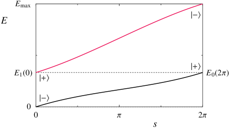
Figure 1: (Color online) Two quasienergies $E_{\pm}(s)$ (bold curves) for the optimal choice of $|{}v{}\rangle$ given at Eq. (13), with $T=1$ and $E_{\rm P}=2\pi/3$. The dashed line corresponds to a unperturbed eigenenergy $E_{1}(0)=E_{\rm P}$. The period of quasienergy space is $E_{\rm max}=2\pi$. The “ground” quasienergy for the present choice of the branch exhibits anholonomy, connecting $E_{0}(s=0)=0$ and $E_{0}(s=2\pi)=E_{\rm P}$. Accordingly the adiabatic passage along the ground quasienergy transports $|{}-{}\rangle$ at $s=0$ to $|{}+{}\rangle$ at $s=2\pi$. Note that the “first excited” quasienergy that connects $(s,E)=(0,E_{\rm P})$ and $(2\pi,E_{\rm max})$ has crossings with other quasienergies (not depicted), which are $s$-independent and, whose eigenspaces are orthogonal to $|{}\pm{}\rangle$ Miyamoto and Tanaka (2007).

The extraordinary speed up by $|{}v{}\rangle$ (13) has to be compensated by the cost for the preparation of the kick part of the Floquet operator $e^{-is|{}v{}\rangle\langle{}v{}|}$, as is mentioned in the previous section. This means that we have to pay the cost to prepare the unitary operator that makes $|{}x{}\rangle$ from a simple state, say, $|{}0{}\rangle^{\otimes n}$. Namely, the effort to solve the given problem by the standard quantum computation is required. In this sense, the present choice of $|{}v{}\rangle$ is not practically useful. However, the present argument is applicable to study the theoretical nature of AAQC, as is shown in Sec V.

IV.2 A “fair” choice of $|{}v{}\rangle$ for Grover’s problem

We first explain the standard adiabatic algorithm Farhi et al. (2000) for Grover’s quantum search Grover (1997) before we examine a fair choice of the state $|{}v{}\rangle$. Let $N$ be the number of items in the unstructured database. The items will be labeled with integers $0,\ldots,N-1$, and the label of the answer is denoted by $x$, which is assumed to be unique. The Hilbert space of the arithmetic register for the standard adiabatic computation is spanned by an orthonormal system $\left\{|{}m{}\rangle\right\}_{m=0}^{N-1}$. The finial Hamiltonian $\hat{H}_{\rm P}$ is a cost function of Grover’s problem:

$$\hat{H}_{\rm P}=\alpha(1-|{}x{}\rangle\langle{}x{}|),$$ (17)

where we introduce an energy scale $\alpha$($>0$). With an initialization of the arithmetic register to be in $|{}0_{\rm B}{}\rangle$, an adiabatic passage along the path of the ground energy of $\hat{H}(s)$, with an adiabatic change of $s$, transposes the state of the arithmetic register to $|{}x{}\rangle$. In SAQC, the minimum gap for the ground energy of $H(s)$ is $\mathcal{O}(N^{-\frac{1}{2}})$ for asymptotically large $N$ Farhi et al. (2000). This implies that the running time is $\mathcal{O}(N)$, if $ds/dt$ is kept constant along the path. Namely, no quantum speedup is available. However, a time-dependent $ds/dt$ introduced by Roland and Cerf provides a Grover-type improvement of running time $\mathcal{O}(\sqrt{N})$, once the locations of narrow gaps in the parameter space could be identified Roland and Cerf (2002). In the latter sense, the standard adiabatic quantum search has the same computational power as the original Grover’s algorithm. We will show that the anholonomic adiabatic approach has the same performance as the standard adiabatic approach.

In the Grover’s problem, we have no prior knowledge of $|{}x{}\rangle$ to choose $|{}v{}\rangle$. Hence, we employ $|{}\mathcal{F}{}\rangle$, which need to have non-zero overlap with $|{}x{}\rangle$, to introduce a normalized $|{}v{}\rangle$:

$$|{}v{}\rangle\equiv a|{}0_{\rm B}{}\rangle\otimes|{}0{}\rangle+b|{}\mathcal{F}{}\rangle\otimes|{}1{}\rangle=a|{}-{}\rangle+b|{}\mathcal{F}{}\rangle\otimes|{}1{}\rangle,$$ (18)

where we choose the phase of $|{}\mathcal{F}{}\rangle$ so that $b$ is positive. Although the overlap $\langle{}x{}|{}\mathcal{F}{}\rangle$ is required to be non-zero, $|\langle{}x{}|{}\mathcal{F}{}\rangle|$ become small as $N\to\infty$, due to the lack of the prior knowledge of $x$ to prepare $|{}\mathcal{F}{}\rangle$. A typical state for $|{}\mathcal{F}{}\rangle$ may be a superposition of all candidates of the answer, that is

$$|{}\mathcal{F}{}\rangle=\frac{1}{\sqrt{N}}\sum_{m=0}^{N-1}|{}m{}\rangle,$$ (19)

in this sense we consider the state $|{}\mathcal{F}{}\rangle$ as a fair choice for $|{}v{}\rangle$. The preparation of $|{}\mathcal{F}{}\rangle$ and hence $|{}v{}\rangle$ is trivial, and hence only polynomially many quantum gates are required to prepare $\hat{U}_{s}$. Hence it is natural to assume $\langle{}x{}|{}\mathcal{F}{}\rangle=\mathcal{O}(N^{-1/2})$ as $N\to\infty$. We introduce a small parameter $\epsilon=\mathcal{O}(N^{-1/2})$ to parameterize the overlap between $|{}x{}\rangle$ and $|{}\mathcal{F}{}\rangle$ as $\langle{}x{}|{}\mathcal{F}{}\rangle=e^{i\theta}\sin\epsilon$, where $0<\epsilon<\pi/2$ and $\theta=\arg\langle{}x{}|{}\mathcal{F}{}\rangle$.

To study the spectrum of $\hat{U}_{s}$, it is convenient to introduce a normalized vector $|{}x^{\perp}{}\rangle\in\mathcal{H}_{\rm A}$:

$$|{}x^{\perp}{}\rangle\equiv\frac{1}{\cos\epsilon}\left(1-|{}x{}\rangle\langle{}x{}|\right)|{}\mathcal{F}{}\rangle.$$ (20)

Hence we have an expansion of $|{}v{}\rangle$ (18) by orthonormal vectors:

$$|{}v{}\rangle=a|{}-{}\rangle+be^{i\theta}\sin\epsilon|{}+{}\rangle+b\cos\epsilon|{}f{}\rangle,$$ (21)

where a normalized vector

$$|{}f{}\rangle\equiv|{}x^{\perp}{}\rangle\otimes|{}1{}\rangle\in\mathcal{H}_{\rm A}\otimes\mathcal{H}_{\rm C}$$ (22)

satisfies $\langle{}\pm{}|{}f{}\rangle=0$.

The subspace spanned by $|{}\pm{}\rangle$ and $|{}f{}\rangle$ is invariant under $\hat{U}_{s}=e^{-i\hat{H}_{0}T}e^{-is|{}v{}\rangle\langle{}v{}|}$ (8) of Grover’s problem. This is because $|{}x^{\perp}{}\rangle$ is an eigenvector of the cost Hamiltonian for Grover’s problem, $\hat{H}_{\rm P}$ (17) and $|{}f{}\rangle$ is accordingly an eigenvector of $\hat{H}_{0}$ (9).

Hence it is suffice to examine a truncation of $\hat{U}_{0}$ by a three-level system

$$\hat{U}_{0}=|{}-{}\rangle\langle{}-{}|+e^{-iE_{\rm P}T}|{}+{}\rangle\langle{}+{}|+e^{-i(E_{\rm P}+\alpha)T}|{}f{}\rangle\langle{}f{}|$$ (23)

for Grover’s problem. The minimum quasienergy gap of $\hat{U}_{s}$ along an increment of $s$ is immediately obtained through numerical diagonalizations of $3\times 3$ unitary matrices (Fig. 2).

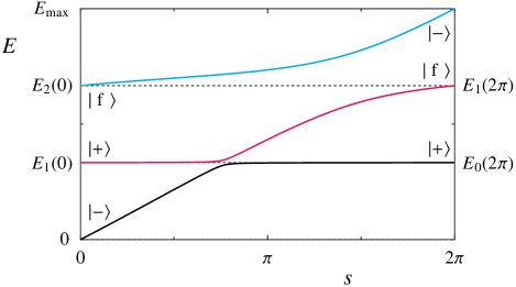
Figure 2: (Color online) Three quasienergies $E_{\pm}(s)$ and $E_{\rm f}(s)$ (bold curves) for the fair choice of $|{}v{}\rangle$ (Eqs. (18) and (19)), with $\left|\langle{}x{}|{}\mathcal{F}{}\rangle\right|^{2}=1/100$ (i.e., $N=100$) and $\left|\langle{}-{}|{}v{}\rangle\right|^{2}=5/6$. The energy scale for the cost Hamiltonian (17) is $\alpha=2\pi/3$. Other parameters are the same as in Fig 1. The adiabatic passage for the computation follows the ground quasienergy $E_{0}(s)$, which encounters a narrow avoided crossing during the increment of $s$ from $0$ to $2\pi$.

We show that the adiabatic passage from $|{}-{}\rangle$ to $|{}+{}\rangle$ encounters a narrow quasienergy gap in Fig. 2, leaving the details of calculation to Appendix A. The magnitude of the gap is $\mathcal{O}(\epsilon)=\mathcal{O}(N^{-1/2})$ by a perturbation expansion by $\epsilon$. An application of Landau-Zener-Stückelberg formula for an estimation of nonadiabatic error implies that the running time of adiabatic approach is $\mathcal{O}(N)$. However, if the location of the quasienergy gap is identified, Roland and Cerf’s prescription Roland and Cerf (2002) is also applicable to the quantum map $\hat{U}_{s}$ to obtain a Grover-type improvement of running time $\mathcal{O}(\sqrt{N})$.

V Efficient simulation of quantum circuits by AAQC

In this section, we will complete to show the equivalence of AAQC with quantum circuits. Since we have already shown that AAQC is efficiently simulated by quantum circuits, we only need to show the converse; quantum circuits can be efficiently simulated by AAQC. To achieve this, we utilize Aharonov et al.’s SAQC  Aharonov et al. (2007) to construct a simulator of a given quantum circuit by AAQC. We remark that their proof for the equivalence of SAQC to quantum circuits can be directory applied to DAQC, since a subset of DAQC consists of all discrete approximant of SAQC, i.e., SAQC is a subset of DAQC in effect. On the other hand, as for AAQC, the relationship with SAQC is not trivial. This is the reason why the equivalence of AAQC to quantum circuits remains nontrivial. The quasienergy gap of our simulator is adjusted by $|{}v{}\rangle$, as is done in Section IV.1, with a reasonable cost for the present case.

Because the following argument involves extensive use of local observables, it is convenient to denote them by local operators, instead of brackets. Let $\mathcal{H}_{\rm b}$ denote the Hilbert space of a qubit and $\left\{|{}0{}\rangle,|{}1{}\rangle\right\}$ corresponding unit vectors. Operators of the qubit are

$$\hat{X}\equiv|{}1{}\rangle\langle{}0{}|+\text{h.c.},\quad\hat{Y}\equiv i|{}1{}\rangle\langle{}0{}|+\text{h.c.},$$

$$\hat{Z}\equiv|{}0{}\rangle\langle{}0{}|-|{}1{}\rangle\langle{}1{}|,$$

$$\hat{{\mathcal{Z}}}\equiv\frac{1}{2}(1+\hat{Z})=|{}0{}\rangle\langle{}0{}|,\quad\hat{{\mathcal{I}}}\equiv\frac{1}{2}(1-\hat{Z})=|{}1{}\rangle\langle{}1{}|.$$ (24)

and we need to introduce “annihilation” and “creation” operators:

$$\hat{A}\equiv|{}0{}\rangle\langle{}1{}|,\quad\hat{A}^{\dagger}\equiv|{}1{}\rangle\langle{}0{}|.$$ (25)

The target of the simulation is a quantum circuit that involves $n$ qubits, whose Hilbert space is denoted by $\mathcal{H}_{\rm A}=(\mathcal{H}_{\rm b})^{\otimes n}$. Let $\hat{a}_{j}^{({\rm A})}$ be a local operator $\hat{a}$ on $j$-th qubit. The quantum circuit is composed by $L$ elementary circuits $\left\{\hat{U}_{l}\right\}_{l=1}^{L}$, where $\hat{U}_{l}$ involves only few (possibly two) qubits, and its state evolves as

$$|{}\alpha(l){}\rangle=\hat{U}_{l}|{}\alpha(l-1){}\rangle.$$ (26)

where the initial and final states of the quantum circuit are $|{}\alpha(0){}\rangle\equiv|{}0{}\rangle^{\otimes n}$ and $|{}\alpha{}\rangle\equiv|{}\alpha(L){}\rangle$, respectively. Our simulator of the quantum circuit by an AAQC depends on the initial and final Hamiltonians $\hat{H}_{\rm B}$ and $\hat{H}_{\rm P}$ of Aharonov et al.’s simulator of the same circuit by a SAQC. Hence the contsruction of these Hamiltonians explained.

Another ingredient of the simulator is Kitaev’s clock Kitaev et al. (2002), which is composed by $L$ qubits. Let $\mathcal{H}_{\rm clock}$ be the Hilbert space of the clock’s states and $\hat{a}_{l}$ be a local operator $\hat{a}$ on clock’s $l$-th qubit. The state of clock at step $l$ is associated with a state

$$|{}c(l){}\rangle\equiv|{}1^{l}0^{L-l}{}\rangle,$$ (27)

which is an eigenstate of $\hat{{\mathcal{I}}}_{1}\hat{{\mathcal{I}}}_{2}\ldots\hat{{\mathcal{I}}}_{l}\hat{{\mathcal{Z}}}_{l+1}\ldots\hat{{\mathcal{Z}}}_{L-1}\hat{{\mathcal{Z}}}_{L}$ with a non-degenerate eigenvalue $1$. Although $\left\{|{}c(l){}\rangle\right\}_{l=0}^{L}$ is orthonormal, it is not a complete system of $\mathcal{H}_{\rm clock}$. Let us introduce a Hilbert space $\mathcal{H}_{\rm clock}^{({\rm V})}$ that is spanned by $\left\{|{}c(l){}\rangle\right\}_{l=0}^{L}$. When the state of the clock does not belong to $\mathcal{H}_{\rm clock}^{({\rm V})}$, the clock is “out of order”. A cost Hamiltonian on $\mathcal{H}_{\rm clock}$

$$\hat{H}_{\rm clock}\equiv\sum_{l=1}^{L-1}\hat{{\mathcal{Z}}}_{l}\hat{{\mathcal{I}}}_{l+1}$$ (28)

is introduced in order to characterize $\mathcal{H}_{\rm clock}^{({\rm V})}$. By definition, the ground subspace of $\hat{H}_{\rm clock}$ is $\mathcal{H}_{\rm clock}^{({\rm V})}$.

Combining Kitaev’s clock and the quantum circuit, the state of the whole system “at $l$-th step” is $|{}\gamma(l){}\rangle\equiv|{}\alpha(l){}\rangle\otimes|{}c(l){}\rangle$. Let $|{}\eta{}\rangle$ be a superposition of $|{}\gamma(l){}\rangle$’s:

$$|{}\eta{}\rangle\equiv\frac{1}{\sqrt{L+1}}\sum_{l=0}^{L}|{}\gamma(l){}\rangle,$$ (29)

which is the destination state, i.e., the ground state of $\hat{H}_{\rm P}$, of Aharonov et al.’s simulator of the quantum circuits. Let $\mathcal{H}_{0}$ be $L$-dimensional Hilbert space spanned by $\left\{|{}\gamma(l){}\rangle\right\}_{l=0}^{L}$. It will be clear that we need to focus on $\mathcal{H}_{0}$ in the following analysis of the simulator.

The initial state of Aharonov et al.’s simulator is $|{}\gamma(0){}\rangle=|{}0{}\rangle^{\otimes(n+L)}$. To achieve this, $\hat{H}_{\rm B}$, the initial Hamiltonian of Aharonov et al.’s SAQC, is composed by three parts. The first ingredient is $\hat{H}_{\rm clock}$ (28), whose ground state must be in $\mathcal{H}_{\rm A}\otimes\mathcal{H}_{\rm clock}^{({\rm V})}$. The next is

$$\hat{H}_{\rm clockinit}\equiv\hat{{\mathcal{I}}}_{1},$$ (30)

whose ground subspace is $\mathcal{H}_{\rm A}\otimes|{}c(0){}\rangle$, if the state space is restricted within $\mathcal{H}_{\rm A}\otimes\mathcal{H}_{\rm clock}^{({\rm V})}$. To initialize the quantum circuit, we introduce

$$\hat{H}_{\rm input}\equiv\left(\sum_{j=1}^{n}\hat{{\mathcal{I}}}^{({\rm A})}_{j}\right)\otimes\hat{{\mathcal{Z}}}_{1},$$ (31)

whose ground subspace contains $|{}\gamma(0){}\rangle$ and $\mathcal{H}_{\rm A}\otimes\left({\rm span}\left\{|{}c(l){}\rangle\right\}_{l=1}^{L}\right)$. To obtain $\hat{H}_{\rm B}$, three Hamiltonians are combined:

$$\hat{H}_{\rm B}\equiv\hat{H}_{\rm clockinit}+\hat{H}_{\rm input}+\hat{H}_{\rm clock},$$ (32)

whose unique ground state is $|{}\gamma(0){}\rangle$.

The finial Hamiltonian $\hat{H}_{\rm P}$ of Aharonov et al.’s SAQC is also composed by three parts. Two of them, $\hat{H}_{\rm input}$ and $\hat{H}_{\rm clock}$, are also contained in $\hat{H}_{\rm B}$. The last part, which we denote $\hat{H}_{\rm h}$, of $\hat{H}_{\rm P}$ is determined so that $|{}\eta{}\rangle$ (Eq. (29)) is a nondegenerate ground state of $\hat{H}_{\rm P}$. A component of $\hat{H}_{\rm h}$, which correspond to the “$l$-th step” of the quantum circuit, is a “five-body” interaction term ($1<l<L$):

$$\hat{H}_{l} \equiv\frac{1}{2}\hat{{\mathcal{I}}}_{l-1}\hat{{\mathcal{Z}}}_{l}\hat{{\mathcal{Z}}}_{l+1}-\frac{1}{2}\left(\hat{{\mathcal{I}}}_{l-1}\hat{U}_{l}\hat{A}^{\dagger}_{l}\hat{{\mathcal{Z}}}_{l+1}+\text{h.c.}\right)$$

$$\quad{}+\frac{1}{2}\hat{{\mathcal{I}}}_{l-1}\hat{{\mathcal{I}}}_{l}\hat{{\mathcal{Z}}}_{l+1}$$ (33)

$$=\hat{{\mathcal{I}}}_{l-1}\hat{h}_{l}\hat{{\mathcal{Z}}}_{l+1},$$ (34)

where the “three-body” term

$$\hat{h}_{l}\equiv\frac{1}{2}\left[1-\left(\hat{U}_{l}\hat{A}^{\dagger}_{l}+\text{h.c.}\right)\right]$$ (35)

transfers $|{}\gamma(l){}\rangle$ into a superposition of $|{}\gamma(l\pm 1){}\rangle$ and the projectors $\hat{{\mathcal{I}}}_{l-1}$ and $\hat{{\mathcal{Z}}}_{l+1}$ make $\hat{H}_{l}$ to be invariant in $\mathcal{H}_{0}$. With the boundary terms

$$\hat{H}_{1}\equiv\hat{h}_{1}\hat{{\mathcal{Z}}}_{2},\quad\text{and}\quad\hat{H}_{L}\equiv\hat{{\mathcal{I}}}_{L-1}\hat{h}_{L},$$ (36)

we have

$$\hat{H}_{\rm h}\equiv\sum_{l=1}^{L}\hat{H}_{l},$$ (37)

which has a unique ground state $|{}\eta{}\rangle$ with the ground energy $0$ and leaves $\mathcal{H}_{0}$ invariant. Hence we obtain the final Hamiltonian

$$\hat{H}_{\rm P}\equiv\hat{H}_{\rm h}+\hat{H}_{\rm input}+\hat{H}_{\rm clock}.$$ (38)

In the following, we employ the restriction of $\hat{H}_{\rm P}$ to $\mathcal{H}_{0}$.

To incorporate Aharanov et al.’s $\hat{H}_{\rm P}$ with the AAQC simulator, we need to estimate the asymptotic behaviors of its energy gap of the ground state and the maximum eigenenergy in the limit $L\to\infty$, within the subspace $\mathcal{H}_{0}$. The spectrum properties of $\hat{H}_{\rm P}$ are also crucial for the Aharonov et al.’s SAQC and are already clarified by them Aharonov et al. (2007). Hence we explain their results only briefly. Since the subspace $\mathcal{H}_{0}$ is an eigenspace of $\hat{H}_{\rm input}+\hat{H}_{\rm clock}$, which is a part of $\hat{H}_{\rm P}$ (see, Eq. (38)), and the corresponding eigenvalue is zero, it is suffice to examine $\hat{H}_{\rm h}$, the nontrivial remainder of $\hat{H}_{\rm P}$. It is straightforward to estimate the spectrum of $\hat{H}_{\rm h}$ from the fact that $\hat{H}_{\rm h}$ is a discretized one-dimensional Laplacian. The first excited energy of $\hat{H}_{\rm P}$ is

$$\Delta=\mathcal{O}(L^{-2})$$ (39)

and is doubly degenerated. The maximum eigenenergy of $\hat{H}_{\rm P}$ is

$$W_{\rm P}=2+\mathcal{O}(L^{-1}).$$ (40)

Hence the two Hamiltonians $\hat{H}_{\rm B}$ and $\hat{H}_{\rm P}$ for Aharonov et al.’s SAQC have introduced.

With these preparations, we introduce an AAQC, which simulates the quantum circuit. The construction of the AAQC from Aharonov et al.’s SAQC follows the prescription explained in Section III. The unperturbed Hamiltonian for the AAQC is

$$\hat{H}_{0}\equiv\hat{H}_{\rm B}{\hat{\mathcal{Z}}}^{({\rm c})}+(\hat{H}_{\rm P}+E_{\rm P}){\hat{\mathcal{I}}}^{({\rm c})}$$ (41)

where ${\hat{\mathcal{Z}}}^{({\rm c})}$ and ${\hat{\mathcal{I}}}^{({\rm c})}$ are projectors of a control register made of a qubit, and $E_{\rm P}$ is non-negative but smaller than $1$, which is the first excited energy of $\hat{H}_{\rm B}$. The ground and the first excited states of $\hat{H}_{0}$ are

$$|{}-{}\rangle\equiv|{}\gamma(0){}\rangle\otimes|{}0{}\rangle=|{}0{}\rangle^{\otimes(n+L+1)}$$ (42)

and

$$|{}+{}\rangle\equiv|{}\eta{}\rangle\otimes|{}1{}\rangle,$$ (43)

respectively, and they are non-degenerate. Our unperturbed Floquet operator is

$$\hat{U}_{0}\equiv e^{-i\hat{H}_{0}T},$$ (44)

where $T$ is the period of our quantum map. Since $\hat{U}_{0}$ is induced by $\hat{H}_{0}$, which is composed only by few-body interactions, $\hat{U}_{0}$ can be implemented efficiently. To ensure that $\hat{U}_{0}$ has no quasienergy between $0<E<E_{\rm P}$, $T$ is assumed to be smaller than $2\pi/W$, where $W$ is the maximum eigenenergy of $\hat{H}_{0}$. From Eq. (40), we have $W=E_{\rm P}+W_{\rm P}=E_{\rm P}+2+\mathcal{O}(L^{-1})$.

To build a quasienergy path that connects between $|{}-{}\rangle$ and $|{}+{}\rangle$ (Eqs. (42) and (43)), we employ

$$|{}v{}\rangle=\frac{1}{\sqrt{2}}(|{}-{}\rangle+|{}+{}\rangle)$$ (45)

to realize quasienergy anholonomy with $N$-independent gap in the Floquet operator

$$\hat{U}_{s}=\hat{U}_{0}e^{-is|{}v{}\rangle\langle{}v{}|}.$$ (46)

It remains to show that the kick part $e^{-is|{}v{}\rangle\langle{}v{}|}$ is efficiently implementable. In the case of Grover’s quantum search, this brings us disastrous slowdown to prepare $|{}v{}\rangle$ (Section IV.1). Contrary to this, we will show that the cost for the preparation of $|{}v{}\rangle$ is negligibly small, in the sense of quantum circuit complexity, to simulate the quantum circuit. The crucial point is to obtain $|{}\eta{}\rangle$ (in $|{}+{}\rangle$) from $|{}\gamma(0){}\rangle$. This is decomposed into two steps. We first introduce a Fourier transformation on $\mathcal{H}_{\rm clock}^{({\rm V})}$ as

$$\hat{F}_{\rm clock}\equiv\sum_{j=0}^{L}|{}c_{j}{}\rangle\langle{}c(j){}|,$$ (47)

where

$$|{}c_{k}{}\rangle\equiv\frac{1}{\sqrt{L+1}}\sum_{l=0}^{L}e^{-i2\pi kl/(L+1)}|{}c(l){}\rangle.$$ (48)

The classical FFT algorithm ensures that the cost of $\hat{F}_{\rm clock}$ is $\mathcal{O}(L\ln L)$ steps. $\hat{F}_{\rm clock}$ acts on $|{}\gamma(0){}\rangle$, yielding

$$\hat{F}_{\rm clock}|{}\gamma(0){}\rangle =\frac{1}{\sqrt{L+1}}|{}\alpha(0){}\rangle\otimes\sum_{l=0}^{L}|{}c(l){}\rangle.$$ (49)

Second, we introduce a “conditional evolution operator”

$$\hat{U}_{\rm h} \equiv\left(\hat{{\mathcal{Z}}}_{L}+\hat{{\mathcal{I}}}_{L}\hat{U}_{L}\right)\left(\hat{{\mathcal{Z}}}_{L-1}+\hat{{\mathcal{I}}}_{L-1}\hat{U}_{L-1}\right)$$

$$\qquad{}\times\cdots\left(\hat{{\mathcal{Z}}}_{1}+\hat{{\mathcal{I}}}_{1}\hat{U}_{1}\right),$$ (50)

which is a product of $L$ few-body unitary operators and is accordingly efficiently implementable. Because its action on $|{}c(l){}\rangle$ extracts a product of quantum circuits as $\hat{U}_{\rm h}|{}c(l){}\rangle=\hat{U}_{l}\hat{U}_{l-1}\cdots\hat{U}_{1}|{}c(l){}\rangle$, it turns out that an efficiently implementable unitary operator $\hat{U}_{\rm h}\hat{F}_{\rm clock}$ gives us $|{}\eta{}\rangle$ from $|{}\gamma(0){}\rangle$

$$\hat{U}_{\rm h}\hat{F}_{\rm clock}|{}\gamma(0){}\rangle=\frac{1}{\sqrt{L+1}}\sum_{l=0}^{L}|{}\gamma(l){}\rangle=|{}\eta{}\rangle.$$ (51)

Hence we have a unitary transformation $\hat{G}$, which makes $|{}v{}\rangle$ from $|{}-{}\rangle$, as follows:

$$\hat{G}=\left({{\mathcal{Z}}}^{({\rm c})}+\hat{U}_{\rm h}\hat{F}_{\rm clock}{{\mathcal{I}}}^{({\rm c})}\right){\hat{H}}^{({\rm c})}$$ (52)

where ${\hat{H}}^{({\rm c})}$ is the Hadamard operation on the control register. Now it is straightforward to see that $\hat{G}$ and the kick operation

$$e^{-is|{}v{}\rangle\langle{}v{}|}=\hat{G}e^{-is|{}-{}\rangle\langle{}-{}|}\hat{G}^{\dagger}$$ (53)

are also efficiently implementable.

Once we build the Floquet operator $\hat{U}_{s}$, $|{}+{}\rangle$ is obtained from $|{}-{}\rangle$, which is easy to prepare, through an adiabatic increment of $s$ from $0$ to $2\pi$ along the adiabatic passage build on Cheon’s quasienergy and eigenspace anholonomies of $\hat{U}_{s}$. Now it is straightforward to obtain $|{}\alpha{}\rangle$, which the final state of the quantum circuit, from $|{}+{}\rangle$ not (e).

To determine the running time of our AAQC, the minimum quasienergy gap along the adiabatic passage needs to be estimated. Due to our choice of $|{}v{}\rangle$, the quasienergy spectrum of $\hat{U}_{s}$ is simple. Two quasienergies depend on $s$. The other quasienergies are independent with $s$, because the corresponding eigenvectors have no overlap with $|{}v{}\rangle$ Miyamoto and Tanaka (2007). Among them, the relevant quasienergy is $E_{\rm P}+\Delta$, which correspond to the first excited energy of $\hat{H}_{\rm P}$. The distance between $E_{\rm P}+\Delta$ and the quasienergy of the adiabatic passage takes minimum value $\Delta$ at $s=2\pi$, at the end of the passage. Hence the minimum gap is $\mathcal{O}(L^{-2})$. Accordingly, the rate of adiabatic change of $s$ needs to be algebraically slow in $L$ to ignore errors due to nonadiabatic transitions. Thus an efficient implementation of the simulator of the quantum circuit is shown to be possible.

VI Summary and outlook

Adiabatic quantum computation that is originally composed of a slowly varying Hamiltonian is reformulated purely in terms of discrete time evolution, e.g. concatenations of quantum circuits, where the concept of quasienergy, instead of eigenenergy, is employed to construct the adiabatic passage. Furthermore, a nontrivial family of DAQC is introduced with the help of the quasienergy anholonomy, which is far more easier to implement than the eigenvalue anholonomy in adiabatic Hamiltonian evolutions. We explain theoretical treatment of AAQC through estimations of quasienergy gaps for “impractical” and “realistic” cases. It turns out that the former case provides a key to show the equivalence of AAQC and the conventional quantum computation. The proof of the equivalence was obtained by extending the proof by Aharonov et al. for SAQC. Although our argument focus only on the essential point of Aharonov et al.’s proof, the rest of sophisticated points could be taken into account straightforwardly for AAQC.

There remains an open question whether AAQC really solves classically intractable problems efficiently. To clarify this, we need to examine AAQC for a hard problem by a classical computer. This certainly involves a simulation of complex quantum dynamics. In this respect, we explain an advantage of AAQC over SAQC from a historical perspective obtained through the studies of classical and quantum chaos Gutzwiller (1990), i.e, prototypes of complex dynamics in classical and quantum mechanics. Although examples of chaos are described by differential equations Lorenz (1963), the discovery of chaotic iterative mapping Hénon (1976); Berry et al. (1979) has galvanized the studies of chaos. This approach allows us to facilitate both numerical and exact analysis Tabor (1989), which can also be applied to adiabatic quantum computation.

Appendix A Estimation of quasienergies for Grover problem with “fair” $|{}v{}\rangle$

We will examine the quasienergies of AAQC’s $\hat{U}_{s}$ (Eq. (8)) for Grover’s problem with the fair choice of $|{}v{}\rangle$ (Eq. (18)), introduced in Sec. IV.2. It is shown above that the subspace spanned by $|{}\pm{}\rangle$ and $|{}f{}\rangle$ (22) is the relevant one for AAQC.

A perturbation expansion with a small parameter $\epsilon$ is suffice to obtain the asymptotic behavior of the minimum quasienergy gap for $N\gg 1$. The reference of the expansion is a unitary operator

$$\hat{W}_{s}\equiv\hat{U}_{0}e^{-is|{}u{}\rangle\langle{}u{}|}$$ (54)

where $|{}u{}\rangle\equiv a|{}-{}\rangle+b|{}f{}\rangle$ agrees with $|{}v{}\rangle$ as $\epsilon\to 0$. Because of the fact $\langle{}u{}|{}+{}\rangle=0$, $|{}+{}\rangle$ is a trivial eigenvector of $\hat{W}_{s}$, in the sense that the corresponding eigenvalue $e^{-iE_{\rm P}T}$ is independent with $s$. Let us denote $|{}w_{-}(s){}\rangle$ and $|{}w_{f}(s){}\rangle$ be the two eigenvectors of $\hat{W}_{s}$ in the remaining subspace spanned by $|{}-{}\rangle$ and $|{}f{}\rangle$, where we impose $|{}w_{-}(0){}\rangle=|{}-{}\rangle$ and $|{}w_{f}(0){}\rangle=|{}f{}\rangle$. The corresponding quasienergies $W_{-}(s)$ and $W_{f}(s)$ are monotonically increase with $s$ and exhibit quasienergy anholonomy: $W_{-}(0)=0\leq W_{-}(s)\leq W_{-}(2\pi)=E_{\rm P}+\alpha=W_{f}(0)\leq W_{f}(s)\leq W_{f}(2\pi)=2\pi/T$. At the same time, two quasienergies $W_{-}(s)$ and $e^{-iE_{\rm P}T}$ of $\hat{W}_{s}$ crosses between $0<s=s_{\rm c}<2\pi$. Hence the adiabatic passages along both $W_{-}(s)$ is inapplicable for the adiabatic search, because the destination of the state vector $|{}f{}\rangle$ does not provide $|{}x{}\rangle$ immediately. Hence we do need to incorporate the effect of small $\epsilon$ to achieve the anholonomic adiabatic quantum search with $\hat{U}_{s}$ (8).

We rearrange $\hat{U}_{s}$ to carry out the perturbation expansion from $\hat{W}_{s}$:

$$\hat{U}_{s}=\hat{W}_{s}\hat{S}_{s},$$ (55)

where

$$\hat{S}_{s}\equiv e^{+is|{}u{}\rangle\langle{}u{}|}e^{-is|{}v{}\rangle\langle{}v{}|}.$$ (56)

The perturbation $\hat{S}_{s}$ makes an exact crossing of the quasienergies $W_{-}(s)$ and $e^{-iE_{\rm P}T}$ of $\hat{W}_{s}$, at $s=s_{\rm c}$, to an avoided crossing of the exact quasienergies $E_{-}(s)$ and $E_{+}(s)$ of $\hat{U}_{s}$. The resultant quasienergy $E_{-}(s)$ connects $|{}-{}\rangle$ at $s=0$ and $|{}+{}\rangle$ at $s=2\pi$. The narrowest quasienergy gap between $E_{-}(s)$ and $E_{+}(s)$ around $s=s_{\rm c}$ determines the speed of the anholonomic quantum search. By using the fact that both $|{}u{}\rangle$ and $|{}v{}\rangle$ belongs to a two-dimensional subspace of $\mathcal{H}_{\rm A}\otimes\mathcal{H}_{\rm C}$, $\hat{S}_{s}$ is expressed as $\hat{S}_{s}=e^{-i\hat{s}_{s}}$, where $\hat{s}_{s}$ is the perturbation “Hamiltonian”

$$\hat{s}_{s}\times\left(\Theta/\sin\Theta\right)^{-1}$$

$$=\left(|{}\delta{}\rangle\langle{}u{}|+|{}u{}\rangle\langle{}\delta{}|+|{}\delta{}\rangle\langle{}\delta{}|\right)\sin{}s$$

$$\quad+i(|{}u{}\rangle\langle{}\delta{}|-|{}\delta{}\rangle\langle{}u{}|)(1-\frac{1}{2}\langle{}\delta{}|{}\delta{}\rangle)\left(1-\cos{}s\right)$$

$$\quad-\left(2|{}u{}\rangle\langle{}u{}|+|{}u{}\rangle\langle{}\delta{}|+|{}\delta{}\rangle\langle{}u{}|\right)\Im(\langle{}u{}|{}\delta{}\rangle)\left(1-\cos{}s\right),$$ (57)

where $|{}\delta{}\rangle\equiv|{}v{}\rangle-|{}u{}\rangle$ and $\Theta$ satisfies

$$\cos\Theta =1-2\left(\langle{}\delta{}|{}\delta{}\rangle-|\langle{}u{}|{}\delta{}\rangle|^{2}\right)\sin^{2}\frac{s}{2}.$$ (58)

From $\langle{}\delta{}|{}\delta{}\rangle=4b^{2}\sin^{2}\frac{\epsilon}{2}$ and $\langle{}u{}|{}\delta{}\rangle=-2b^{2}\sin^{2}\frac{\epsilon}{2}$, we have

$$\cos\Theta =1-8b^{2}\sin^{2}\frac{\epsilon}{2}\left(1-b^{2}\sin^{2}\frac{\epsilon}{2}\right)\sin^{2}\frac{s}{2}.$$ (59)

Hence, in the asymptotic regime $|\epsilon|\ll 1$, we obtain $\Theta/\sin\Theta=1+\mathcal{O}(\epsilon^{2})$. Finally, we obtain the leading contribution of $\hat{s}_{s}$ with respect to an expansion by $\epsilon$:

$$\hat{s}_{s}=2\epsilon b\sin\frac{s}{2}\left(|{}+{}\rangle\langle{}u{}|e^{i\theta-is/2}+\text{h.c.}\right)+\mathcal{O}(\epsilon^{2}).$$ (60)

Thus we conclude that, if we avoid $s_{c}=0,\pi$, the minimum quasienergy gap between $E_{-}(s)$ and $E_{+}(s)$ is $|2\epsilon b\sin(s_{c}/2)|=\mathcal{O}(\epsilon)$.

References

- Messiah (1999) A. Messiah, Quantum Mechanics (Dover, New York, 1999), chap. 17.
- Farhi et al. (2000) E. Farhi, J. Goldstone, S. Gutmann, and M. Sipser (2000), eprint arXiv:quant-ph/0001106.
- Aharonov et al. (2007) D. Aharonov, W. van Dam, J. Kempe, Z. Landau, and S. Lloyd, SIAM Journal on Computing 37, 166 (2007).
- Farhi et al. (2001) E. Farhi, J. Goldstone, S. Gutmann, J. Lapan, A. Lundgren, and D. Preda, Science 292, 472 (2001).
- Schützhold and Schaller (2006) R. Schützhold and G. Schaller, Phys. Rev. A 74, 060304 (2006).
- Žnidarič (2005) M. Žnidarič, Phys. Rev. A 71, 062305 (2005).
- Žnidarič and Horvat (2005) M. Žnidarič and M. Horvat, Phys. Rev. A 73, 022329 (2005).
- Farhi et al. (2008) E. Farhi, J. Goldstone, S. Gutmann, and D. Nagaj, Int. J. Quantum Info. 6, 503 (2008), eprint arXiv:quant-ph/0512159.
- Hogg (2003) T. Hogg, Phys. Rev. A 67, 022314 (2003).
- not (a) We do not claim that any realization of SAQC requires the discretization. See, e.g., a proposal of an implementation with STIRAP [D. Daems and S. Guérin, Phys. Rev. Lett. 99, 170503 (2007)].
- Steffen et al. (2003) M. Steffen, W. van Dam, T. Hogg, G. Breyta, and I. Chuang, Phys. Rev. Lett. 90, 067903 (2003).
- Zel’dovich (1967) Y. B. Zel’dovich, Sov. Phys.–JETP 24, 1006 (1967).
- Tanaka and Miyamoto (2007) A. Tanaka and M. Miyamoto, Phys. Rev. Lett. 98, 160407 (2007).
- Cheon and Tanaka (2009) T. Cheon and A. Tanaka, Europhys. Lett. 85, 20001 (2009).
- Cheon (1998) T. Cheon, Physics Letters A 248, 285 (1998).
- Miyamoto and Tanaka (2007) M. Miyamoto and A. Tanaka, Phys. Rev. A 76, 042115 (2007).
- Grover (1997) L. K. Grover, Phys. Rev. Lett. 79, 325 (1997).
- Berry et al. (1979) M. Berry, N. Balazs, M. Tabor, and A. Voros, Ann. Phys. 122, 26 (1979).
- Lloyd (1996) S. Lloyd, Science 273, 1073 (1996).
- not (b) Our definition of eigenangle and the conventional one have opposite sign. This is to make a natural correspondence with quasienergy and the time development of dynamical phase.
- Nakamura (2002) H. Nakamura, Nonadiabatic transition (World Scientific, Singapore, 2002), and references therein.
- Breuer and Holthaus (1989) H. Breuer and M. Holthaus, Z. Phys. D 11, 1 (1989).
- not (c) Note that and are also neighboring eigenenergy of in the unit circle, due to the condition .
- not (d) If is the maximum eigenenergy of , is the ground energy due to the periodicity of quasienergy space.
- Roland and Cerf (2002) J. Roland and N. J. Cerf, Phys. Rev. A 65, 042308 (2002).
- Kitaev et al. (2002) A. Y. Kitaev, A. H. Shen, and M. N. Vyalyi, Classical and Quantum Computation (American Mathematical Society, Providence, RI, 2002).
- not (e) To obtain from a single measurement of , with reasonably small overhead and errors, it is suffice to employ Aharonov et al.’s amplification technique that increases the weight of in (see Lemma 3.10 in Ref. Aharonov et al. (2007)).
- Gutzwiller (1990) M. C. Gutzwiller, Chaos in Classical and Quantum Mechanics (Springer-Verlag, New York, 1990).
- Lorenz (1963) E. N. Lorenz, J. Atmos. Sci. 20, 130 (1963).
- Hénon (1976) M. Hénon, Comm. Math. Phys. 50, 69 (1976).
- Tabor (1989) M. Tabor, Chaos and integrability in nonlinear dynamics: an introduction (Wiley, New York, 1989).