Frequentist comparison of CMB local extrema statistics in the five-year WMAP data with two anisotropic cosmological models

Abstract

We present local extrema studies of two models that introduce a preferred direction into the observed cosmic microwave background (CMB) temperature field. In particular, we make a frequentist comparison of the one- and two-point statistics for the dipole modulation and ACW models with data from the five-year Wilkinson Microwave Anisotropy Probe (WMAP). This analysis is motivated by previously revealed anomalies in the WMAP data, and particularly the difference in the statistical nature of the temperature anisotropies when analysed in hemispherical partitions.

The analysis of the one-point statistics indicates that the previously determined hemispherical variance difficulties can be apparently overcome by a dipole modulation field, but new inconsistencies arise if the mean and the $\ell$-dependence of the statistics are considered. The two-point correlation functions of the local extrema, $\xi_{\rm TT}$ (the temperature pair product) and $\xi_{\rm PP}$ (point-point spatial pair-count), demonstrate that the impact of such a modulation is to over-‘asymmetrise’ the temperature field on smaller scales than the wave-length of the dipole or quadrupole, and this is disfavored by the observed data. The results from the ACW model predictions, however, are consistent with the standard isotropic hypothesis. The two-point analysis confirms that the impact of this type of violation of isotropy on the temperature extrema statistics is relatively weak.

From this work, we conclude that a model with more spatial structure than the dipole modulated or rotational-invariance breaking models are required to fully explain the observed large-scale anomalies in the WMAP data.

1 Introduction

Local extrema in the CMB have been extensively studied in the context of hotspots (peaks) and coldspots (troughs) arising in Gaussian random fields (Bond & Efstathiou, 1987; Vittorio & Juszkiewicz, 1987). Additional statistics related to such local extrema, such as the Gaussian curvature and temperature-correlation function, have been investigated as a means to distinguish the geometry of the universe and test the Gaussian hypothesis for the nature of the initial conditions (Barreiro et al., 1997; Heavens & Sheth, 1999; Heavens & Gupta, 2001). Such statistical techniques have subsequently been applied to several datasets, and most notably by Kogut et al. (1995, 1996) with the $COBE$-DMR data. Observations from the Wilkinson Microwave Anisotropy Probe (WMAP) currently provide the most comprehensive, full-sky, high-resolution CMB measurements to-date, and studies on the local extrema properties thereof have been undertaken (Larson & Wandelt, 2004, 2005; Tojeiro et al., 2006).

More recently in Hou, Banday & Górski (2009), we extensively analyzed the statistical properties of both the one- and two-point statistics of local extrema in the five-year WMAP temperature data. Such extrema are defined as those pixels whose temperature values are higher (maxima) or lower (minima) than all of the adjacent pixels (Wandelt, Hivon & Górski, 1998). We considered only that part of the sky outside of the WMAP KQ75 mask and its subsequent partition in either Galactic or Ecliptic coordinates into northern and southern hemispheres (hereafter GN, GS, EN, ES). A frequentist comparison with the predictions of a Gaussian isotropic cosmological model that adopted the best-fit parameters from the WMAP team was then made. The hypothesis test indicated a low-variance of both local maxima and minima in the Q-, V- and W-band data that was inconsistent with the Gaussian hypothesis at the 95% C.L. The two-point analysis showed that the observed temperature pair product at a given threshold $\nu$, $\xi_{\rm TT}(\theta,\nu>1,2)$, indicates a $3\sigma$ level ‘suppression’ on GN and EN, whereas $\xi_{\rm TT}(\theta<20^{\circ},\nu<\infty)$ is suppressed on the full-sky and both northern hemisphere partitions. The latter is also the case for the point-point spatial pair-count function $\xi_{\rm PP}(\theta<20^{\circ},\nu>1,2)$. Intriguingly, the statistics showed an $\ell$-dependence such that consistency with the Gaussian hypothesis was achieved once the first 5 or 10 best-fitting multipoles were subtracted, implying that the anomalies may be connected to features of the large-scale multipoles.

The local extrema anomalies therefore provide further evidence of a hemispherical asymmetry that was originally revealed using the power spectrum (Hansen, Banday & Górski, 2004; Eriksen et al., 2004; Hansen et al., 2008), the N-point correlation functions (Eriksen et al., 2005) and Minkowski functionals (Park C-G, 2004). This can be interpreted as a violation of the cosmological principle of isotropy. Theoretically, Gordon et al. (2005) proposed a mechanism of spontaneous isotropy breaking in which the long-wavelength modes of a mediating field couple non-linearly to the CMB perturbations. These fluctuations appear locally as a gradient and imprint a preferred direction on the sky. An implementation of a multiplicative modulation field of the intrinsic anisotropy with a single preferred direction was fitted to the three-year WMAP observations in Eriksen et al. (2007) . The so-called ‘dipole modulation field’ (dmf) was detected at a significant confidence level, and confirmed at even higher significance in the five-year WMAP data by Hoftuft et al. (2009).

Another mechanism that violates rotational invariance was proposed by Ackerman, Carroll & Wise (2007). The ACW model picks out a preferred direction during cosmological inflation to modify the power spectrum of primordial perturbations, $P(k)$. Its imprint on the CMB can then be described by the covariance matrix of spherical harmonic coefficients, $\langle a_{\ell m}a^{*}_{\ell^{\prime}m^{\prime}}\rangle$. Groeneboom & Eriksen (2009) estimated the parameters of the ACW model in an extended CMB Gibbs sampling framework from the five-year WMAP data. The posterior distribution of the parameters indicated a convincing detection of isotropy violation at $3.8\sigma$ significance in the W-band data.

In this paper, we make a frequentist comparison of the dmf and ACW models with the five-year WMAP maps of temperature anisotropy using a large number of Monte-Carlo simulations. In particular, we consider the one- and two-point statistics of local extrema and evaluate whether the WMAP data are more consistent with these models as opposed to the standard Gaussian cosmological models against which various anomalies have been claimed. A rigorous hypothesis test methodology is applied to establish the significance at which the models impact the previous conclusions regarding WMAP data and the violation of isotropy. In addition, the $\xi_{\rm TT}$ and $\xi_{\rm PP}$ correlation functions are utilised to further confirm the findings of the one-point analysis and to study the scale-dependence of the local extrema both in real and spherical harmonic space.

It might be considered that the statistical significance of the local extrema anomalies alone is insufficient to warrant an analysis of the anisotropic models, in particular given the additional parameters required to specify them. However, that they provide significantly better fits to the WMAP data than the isotropic model has been demonstrated by independent Bayesian power spectrum analysis. It is clearly then quite legitimate to consider the local extrema statistics in terms of these improved models, and to determine whether the observed local extrema are also more consistent with such cosmological prescriptions. In fact, we will find that there is little evidence that the extrema anomalies are remedied by these models, and indeed in one case we show that the anomalous behaviour becomes more significant.

This paper is organised as follows. In Section 2.1, we present an overview of the WMAP data and the instrumental properties that must be involved in Gaussian simulations to enable an unbiased comparison with the real data. The two models and the algorithms for simulating them are briefly reviewed in Section 2.2. Section 2.3 prescribes the technique used for further data-processing and introduces the one- and two-point analysis methods. The results are reported in Section 3 before we present our conclusions in Section 4.

2 METHOD

Both the dipole modulation and ACW models provide mechanisms for the violation of cosmological isotropy in the context of Gaussian random fields. In a frequentist formalism, we construct simulations for each model, convolve with the appropriate instrumental beam transfer functions, then add noise according to the properties of the WMAP detectors. The statistical properties of the simulated data are then compared with the observed ones to verify the consistency of the models with the observed Universe.

2.1 The WMAP data

The WMAP instrument consists of 10 differencing assemblies (DAs) covering frequencies from 23 to 94 GHz (Bennett et al., 2003). The V and W-band foreground-reduced sky maps are used in our analysis, consistent with the data selection for the WMAP five-year power spectrum estimation (Nolta et al., 2009). The maps are available in the HEALPix pixelisation scheme with $N_{\rm side}=512$ from the LAMBDA website. We combine data from DAs covering the same frequency using uniform weighting over the sky and equal weight per DA. This allows a simple effective beam to be computed from the combination of beam transfer functions ($b_{\ell}$) for the DAs involved. In fact, the WMAP beams are not axisymmetric and Wehus et al. (2009) have attempted to assess the effect of the combination of the true asymmetric beams with scanning strategy on the sky using reconstructed sky maps. They report deviations from the official $b_{\ell}$ at a level of $\approx$1.0% at $\ell\approx 800$. However, the additional smoothing employed in this work render our statistics insensitive to such deviations, thus we continue to adopt the beam properties provided by the WMAP team. There are two noise components contributing to observations, white noise and residual $1/f$ noise following an effective destriping in the map-making process. However, the $1/f$ noise can be considered negligible even on the largest scales since the 5-year signal-to-noise level is so high (Hinshaw et al., 2007).

The extended temperature analysis mask (KQ75 which leaves approximately 72% sky usable coverage) is applied to the data to eliminate regions contaminated by Galactic foreground and point sources. Hemispherical masks of the Galactic North and South (GN and GS), Ecliptic North and South (EN and ES) are also applied together with the KQ75 mask for some parts of our analysis. In this paper, we will refer to results derived on the KQ75 sky-coverage as ‘full-sky’ results for convenience, to distinguish then from the corresponding results on masked hemispheres.

2.2 The two models

In this section, we briefly review the implementation of the two models discussed in our work. We use $T^{\prime}_{\rm{dmf}}$ and $T^{\prime}_{\rm{acw}}$ to identify the simulated realisations for each model, which are then combined with the beam profiles and WMAP-like noise properties for each frequency band concerned in the analysis. The realisations are performed at a HEALPix resolution parameter $N_{\rm side}=512$ with maximum multipole, $\ell_{\rm max}=1024$.

2.2.1 Dipole modulation

We follow Eriksen et al. (2007) and their implementation of a multiplicative dipole modulation field as proposed in Gordon et al. (2005).

The CMB temperature field is defined as

$$\tilde{T}(\textbf{{n}})=T(\textbf{{n}})[1+f(\textbf{{n}})],$$ (1)

where $T(\textbf{{n}})=\sum_{\ell,m}a_{\ell m}Y_{\ell m}(\textbf{{n}})$ is a statistically isotropic CMB temperature field with power spectrum $C_{\ell}$ and $f(\textbf{{n}})$ is a dipole modulation field with amplitude much less than one but non-zero.

In their low $\ell$ analysis of the WMAP data, Eriksen et al. (2007) have parameterised the dmf model using four free parameters, $q$ (normalisation amplitude), $n$ (tilt), $A$ (amplitude of dmf) and p (direction of dmf), together with a fiducial Gaussian power-spectrum, $C_{\ell}^{\rm fid}$, which was chosen to be the WMAP best-fitting power spectrum. The power spectrum and modulation field are then written as

$$C_{\ell;(q,n)}=q\left(\frac{\ell}{\ell_{0}}\right)^{n}C_{\ell}^{\rm fid}\ {\rm{and}}\ f(\textbf{{n}};A,\textbf{{p}})=A\textbf{{n}}\cdot\textbf{{p}}.$$ (2)

In fact, this formalism recognises that the best-fitting dmf may also impact other cosmological parameters, but that over the limited range in $\ell$ that the analysis is carried out, the practical effect can be represented by a normalisation $q$ and spectral tilt $n$. The posterior distributions of the parameters were then given by an optimal Bayesian analysis.

In this work, we modulate Gaussian realisations of the CMB adopting the most recent parameters estimated from the WMAP5 data in Hoftuft et al. (2009). Their estimations seem to provide a robust value of p, whereas the magnitude $A$ seems to be a function of $\ell_{\rm mod}$, the maximum value of $\ell$ included in the analysis. We therefore simulate the dmf adopting the best-fitting directions for the different $\ell_{\rm mod}$ ranges, and consider values for the amplitude $A$ varying spanning the 68% confidence region for each range. These parameters sets are summarised in Table 1. Note that we apply these parameters over the full range of $\ell$ used in the simulations. Importantly, they find that $q$ and $n$ are consistent with unity and zero respectively (for the V-band, the actual values are $q=0.96\pm 0.05$ and $n=0.06\pm 0.05$), thus we can simply assume the WMAP5 best-fitting ‘lcdm+sz+lens’ model power spectrum as our fiducial spectrum, and that the presence of the dmf does not perturb the best-fit cosmological parameters.

Table 1: The groups of parameters adopted for the dmf simulations. The $(A,\textbf{{p}})$ values are estimated by Hoftuft et al. (2009) for different maximum values of multipole moment, $\ell_{\rm mod}$, involved during the estimation. The dipole axis p point towards $(l,b)$ in Galactic coordinates.

Band	$\ell_{\rm mod}$	$A$	$\textbf{{p}}(l,b)$
V	40	$0.119-0.034$	$(224^{\circ},-22^{\circ})$
		0.119
		$0.119+0.034$
	64	$0.080-0.021$	$(232^{\circ},-22^{\circ})$
		$0.080$
		$0.080+0.021$
	80	$0.070-0.019$	$(235^{\circ},-17^{\circ})$
		$0.070$
		$0.070+0.019$
W	64	$0.074-0.021$	$(232^{\circ},-22^{\circ})$
		$0.074$
		$0.074+0.021$

The simulated realisations $T^{\prime}_{\rm dmf}(\textbf{{n}})$ are then given by

$$\tilde{a}_{\ell m} =\,b_{\ell}\sum_{\textbf{{n}}}\tilde{T}(\textbf{{n}})Y_{\ell m}(\textbf{{n}}),$$ (3)

$$T^{\prime}_{\rm dm}(\textbf{{n}}) =\,\sum_{\ell,m}\tilde{a}_{\ell m}Y_{\ell m}(\textbf{{n}})+N(\textbf{{n}}).$$ (4)

These realisations are then convolved with the appropriate beam transfer function $b_{\ell}$, and noise realisations $N(\textbf{{n}})$ are added. For each group of $(A,\textbf{{p}})$, we perform 2500 simulations for comparison with observations.

2.2.2 The ACW model

Inflationary theory gives a firm prediction that the primordial density perturbations should be isotropic without any preferred direction. Ackerman, Carroll & Wise (2007) considered the breaking of this rotational invariance by the explicit introduction of a preferred direction, $\textbf{{n}}^{\prime}$, during the inflationary era thus modifying the primordial power spectrum $P(k)$ to

$$P^{\prime}(\textbf{{k}};g(k),\textbf{{n}}^{\prime})=P(k)[1+g(k)(\textbf{{k}}\cdot\textbf{{n}}^{\prime}/k)^{2}],$$ (5)

where k is the vector with magnitude $k$. $g(k)$ is a general function representing the rotationally non-invariant part, which ACW have argued can be approximated by a constant $g_{*}$. The imprint of this preferred direction on the CMB is then given by

$$S_{\ell m,\ell^{\prime}m^{\prime}}=\langle a_{\ell m}a^{*}_{\ell^{\prime}m^{\prime}}\rangle=C_{\ell}\delta_{\ell\ell^{\prime}}\delta_{mm^{\prime}}+\Delta_{\ell m,\ell^{\prime}m^{\prime}},$$ (6)

where $C_{\ell}$ is the CMB angular power spectrum and we define

$$\Delta_{\ell m,\ell^{\prime}m^{\prime}}=g_{*}\xi_{\ell m,\ell^{\prime}m^{\prime}}\int^{\infty}_{0}dk\,k^{2}P(k)\Theta_{\ell}(k)\Theta_{\ell^{\prime}}(k).$$ (7)

$\xi_{\ell m,\ell^{\prime}m^{\prime}}$ are then geometric factors that describe coupling between modes, $\ell$ to $\ell^{\prime}=\ell,\ell+2$ and $m$ to $m^{\prime}=m,m\pm 1,m\pm 2$. The integral term is a generalisation of the standard CMB power spectrum and may be computed using a modified version of CAMB (Lewis, Challinor & Lasenby, 2000).

The contribution of $\Delta$ can contribute significantly to the diagonal part of S which affects the total angular power spectrum and induces strong degeneracy between $g_{*}$ and the amplitude of the power spectrum of scalar perturbations, $A_{s}$. However, it can be ensured that a given choice of $g_{*}$ mainly affects the anisotropic contribution by redefining the signal covariance matrix. as

$$S_{\ell m,\ell^{\prime}m^{\prime}}=\frac{C_{\ell}\delta_{\ell\ell^{\prime}}\delta_{mm^{\prime}}+\Delta_{\ell m,\ell^{\prime}m^{\prime}}}{1+g_{*}/3},$$ (8)

In this work, we assume that the cosmological parameters are known and given by the WMAP5 best-fitting ‘lcdm+sz+lens’ model power spectrum (Komatsu et al., 2009). The two free parameters remaining in the model, $(g_{*},\textbf{{n}}^{\prime})$, have been estimated by Groeneboom & Eriksen (2009) from the WMAP five-year data using Bayesian analysis in an extended CMB Gibbs sampling framework. The estimation was carried out over different $\ell$-ranges to investigate whether the preferred direction $\textbf{{n}}^{\prime}$ is dependent on the $\ell$-range selection. Indeed, a preferred direction and value for $g_{*}$ for the ACW model was found for the V and W-bands at $2.5\sigma$ and $3.8\sigma$ confidence-level, respectively (Table 1 of their paper), although there is a $20^{\circ}$ deviation in Galactic longitude between the two bands. For the range $\ell=[2,400]$ and KQ85 sky-coverage, the $g_{*}$ value is reported as $0.10\pm 0.04$ for the V-band and $0.15\pm 0.039$ for W-band (95% confidence), while for the more conservative KQ75 sky-coverage the V-band $g_{*}$ value is $0.10[-0.100,0.158]$. In Hou, Banday & Górski (2009), we show that the signal-to-noise-ratio (S/N) of the 5-year WMAP temperature data decreases to 1 at $\ell=399$ (385) on V- (W-) band, and the additional smoothing imposed during data-processing suppresses information on this scale by a further factor of 0.1 in spherical harmonic space. Therefore, we choose different $g_{*}$ values estimated from the $\ell$-range [2,400] within the 95% confidence region, to carry out the frequentist comparison. The parameters used in this work are summarised in Table 2.

Table 2: The groups of parameters used in our local extrema analysis for ACW model. The parameters follow the estimation results of Groeneboom & Eriksen (2009) for $\ell$-range [2,400].

V-band		W-band
$g_{*}$	$\textbf{{n}}^{\prime}(l,b)$	$g_{*}$	$\textbf{{n}}^{\prime}(l,b)$
-0.100	$(130^{\circ},10^{\circ})$	0.111	$(110^{\circ},10^{\circ})$
-0.050		0.130
0.050		0.150
0.100		0.170
0.158		0.189
0.158	$(110^{\circ},10^{\circ})$	0.189	$(130^{\circ},10^{\circ})$

We then follow the algorithm of Groeneboom & Eriksen (2009) to get the simulated ACW realisations of the sky using

$$T^{\prime}_{\rm acw}(\textbf{{n}};g_{*},\textbf{{n}}^{\prime}) = \sum_{\ell,m}b_{\ell}2^{\frac{\delta_{m0}-1}{2}}L_{\ell m}(g_{*},\textbf{{n}}^{\prime})\eta_{\ell m}Y_{\ell m}(\textbf{{n}})$$ (9)

$$\mbox{}+N(\textbf{{n}}),$$

where $L_{\ell m}$ is the Cholesky decomposition of the sparse covariance matrix S, involving the best-fitting parameters $(g_{*},\textbf{{n}}^{\prime})$ and cosmological model, and $\eta_{\ell m}$ is a set of Gaussian random numbers with zero mean and unit variance. The factor $2^{\frac{\delta_{m0}-1}{2}}$ is placed regarding the triangular $L_{\ell m}$ and HEALPix data convention. Each simulation is convolved with the appropriate WMAP beams and noise realisations are added. For each group of parameters, we perform 5000 simulations.

2.3 Analysis and statistics

In this section, we introduce the processing steps and statistics utilised for the local extrema comparison between the observed sky and simulations for our two selected models. Generally, the treatment follows closely that of sections 2.5 and 2.6 of Hou, Banday & Górski (2009), but is briefly reviewed here.

The data and simulations are treated in an identical way. Masks are applied to the sky maps, then the best-fitting monopole and dipole components for the region outside the mask are subtracted – this is a standard procedure in CMB data analysis. Since our previous results on local extrema statistics suggest a close connection with large angular scale modes on the sky, we also consider cases where modes up to and including the quadrupole, $\ell\leq 5$ or $\ell\leq 10$ are also subtracted before analysis. A modest smoothing is then applied to the resulting sky maps where the angular scale of smoothing is determined by a signal-to-noise normalisation technique. In this work, we applied 43.485 arcmin and 45.064 arcmin FWHM Gaussian beams to the masked sky maps of the V- and W-band respectively. In order to be conservative and avoid potential boundary effects in the analysis, the masks (for which all valid pixels are set to unity) are also smoothed and only those pixels with values larger than 0.90 are retained as valid. The local extrema are then determined using the hotspots program in the HEALPix package.

First, the one-point statistics (number, mean, variance, skewness and kurtosis) of the local extrema temperature distribution are computed for further hypothesis test. The hypothesis test methodology introduced by Larson & Wandelt (2005) is again adopted here. The probability of finding a simulated statistic that falls below the observed one is defined as $p$. As a two-sided test, we set the significance level $\alpha=0.05$ with the hypothesis

$$H:p\in(\alpha/2,1-\alpha/2),$$ (10)

and perform the test twice to control the Type I error ($\beta$ – rejection of true hypothesis) and the Type II error ($\gamma$ – acceptance of the false hypothesis) to be small.

Secondly, the two-point correlation functions of temperature pairs, $\xi_{\rm TT}$, and spatial pair-counting, $\xi_{\rm PP}$, are computed to make a further $\chi^{2}$ analysis. During the two-point analysis, each realisation can be examined in a renormalised form, $T(\textbf{{n}})=\nu(\textbf{{n}})\sigma_{\rm sky}$, where $\sigma_{\rm sky}$ is the standard-deviation of the temperature field over the valid region of each realisation. We will continue to examine the correlation dependence on the thresholds $\nu$,e and the large-scale multipoles. For the $\xi_{\rm PP}$ computation, we utilise the Hamilton estimator (Hamilton, 1993) and use the same random sample as in Hou, Banday & Górski (2009). Since the $\{\xi_{\rm TT}(\theta)\}$ and $\{\xi_{\rm PP}(\theta)\}$ are asymmetrically distributed in a given angular range, the $\chi^{2}$ statistics are optimised by mapping the distributions to Gaussian ones $\{s(\theta)\}$,

$$\frac{\rm Rank\ of\ observed\ map}{\rm{Total\ number\ of\ maps}+1}=\frac{1}{\sqrt{2\pi}}\int_{-\infty}^{s}e^{-\frac{1}{2}t^{2}}\,dt.$$ (11)

Then the probability of finding the number of simulations with a $\chi^{2}$ value below the observed one can be determined.

3 RESULTS AND DISCUSSIONS

In this paper, we will not attempt to describe all the one- and two-point results determined, but instead highlight some interesting cases that help to build the conclusions.

Those results that are derived after subtraction of the low–$\ell$ multipoles in the range $[0,\ell_{\rm rmv}]$ are denoted by $\ell_{\rm rmv}$ for simplicity, where $\ell_{\rm rmv}=1$, 2, 5 and 10.

In the frequentist comparison, we determine the probability $p$ described in section 2.3 by counting the number of simulations with statistical values (either one-point statistics or the associated $\chi^{2}$ measure for the two-point analysis) below the observed one. For the one-point analysis, the probabilities are subjected to a hypothesis test twice, the first test sets $\beta=\alpha$ and any rejections are listed in the tables and marked by asterisks; the second test sets $\gamma=\alpha$, with the subsequent rejections that were accepted by the first test marked by question-marks. If we specify $\alpha=0.05$, those cases rejected by the first test indicate that the consistency of the observations with the model concerned is rejected at the 95% C.L., with an associated 5% probability of a Type I error ($\beta=0.05$). For those cases accepted by the second test, it can then be asserted that such a consistency is accepted at the 0.05 significance level, with an associated 5% probability of a Type II error ($\gamma=0.05$).

3.1 Dipole modulation results

A subset of the results are shown in Table 3. We only present the local extrema mean and variance statistics for $\rm V^{A=0.119\pm 0.034}_{\textbf{{p}}=(224^{\circ},-22^{\circ})}$ and $\rm W^{A=0.074\pm 0.021}_{\textbf{{p}}=(232^{\circ},-22^{\circ})}$ here, since the number, skewness and kurtosis values are not revealing, and the results from other groups of dmf parameters lead to similar conclusions.

Table 3: Frequencies of the extrema one-point statistics with lower values than the WMAP V and W-band five-year data. The dmf parameters are given as superscripts and subscripts of the frequency label. The local maxima (minima) results are denoted as ‘max’ (‘min’). NS, GN, GS, EN and ES correspond to full-sky, Galactic North, Galactic South, Ecliptic North and Ecliptic South sky-coverage outside of the KQ75 mask, respectively. The values rejected by the hypothesis test are marked by a * or ?. Values outside the $3\sigma$ confidence range are underlined.

WMAP5, KQ75		NS	GN	GS	EN	ES	NS	GN	GS	EN	ES
MEAN		$\ell_{\rm rmv}=1$					$\ell_{\rm rmv}=2$
$\rm V^{A=0.085}_{(224^{\circ},-22^{\circ})}$	max	0.1416	0.5252	0.0604	0.8584	0.0052*	0.1436	0.8776	0.0600	0.9628	0.0000*
	min	0.0908	0.3908	0.0592	0.7980	0.0016*	0.1304	0.3040	0.0596	0.8720	0.0008*
$\rm V^{A=0.119}_{(224^{\circ},-22^{\circ})}$	max	0.1216	0.5816	0.0392	0.8292	0.0064*	0.1248	0.9088	0.0284?	0.9468	0.0000*
	min	0.0812	0.4460	0.0376	0.7632	0.0012*	0.1108	0.3616	0.0324	0.8408	0.0012*
$\rm V^{A=0.153}_{(224^{\circ},-22^{\circ})}$	max	0.1312	0.8340	0.0060*	0.9940*	0.0000*	0.1340	0.9856*	0.0060*	0.9992*	0.0000*
	min	0.0860	0.7536	0.0084*	0.9892*	0.0000*	0.1180	0.6820	0.0068*	0.9988*	0.0000*
		$\ell_{\rm rmv}=5$					$\ell_{\rm rmv}=10$
$\rm V^{A=0.085}_{(224^{\circ},-22^{\circ})}$	max	0.4056	0.9640	0.0164*	0.9836*	0.0008*	0.4168	0.9076	0.0260?	0.9988*	0.0000*
	min	0.0596	0.3064	0.0328	0.9272	0.0004*	0.0944	0.6784	0.0396	0.9656	0.0004*
$\rm V^{A=0.119}_{(224^{\circ},-22^{\circ})}$	max	0.3700	0.9748?	0.0080*	0.9760?	0.0008*	0.4072	0.9684	0.0044*	1.0000*	0.0000*
	min	0.0476	0.3648	0.0148*	0.8968	0.0000*	0.0916	0.8520	0.0108*	0.9984*	0.0000*
$\rm V^{A=0.153}_{(224^{\circ},-22^{\circ})}$	max	0.3900	0.9976*	0.0004*	1.0000*	0.0000*	0.4024	0.9940*	0.0008*	1.0000*	0.0000*
	min	0.0532	0.7076	0.0020*	0.9992*	0.0000*	0.0888	0.9468	0.0024*	1.0000*	0.0000*
		$\ell_{\rm rmv}=1$					$\ell_{\rm rmv}=2$
$\rm W^{A=0.053}_{(232^{\circ},-22^{\circ})}$	max	0.1800	0.4380	0.1296	0.8904	0.0136*	0.1528	0.7380	0.1036	0.9556	0.0068*
	min	0.0632	0.0860	0.1756	0.5716	0.0068*	0.0704	0.0476	0.1984	0.6148	0.0116
$\rm W^{A=0.074}_{(232^{\circ},-22^{\circ})}$	max	0.1760	0.5524	0.0852	0.9608	0.0028*	0.1524	0.8244	0.0568	0.9884*	0.0004*
	min	0.0624	0.1408	0.1076	0.7664	0.0012*	0.0700	0.0816	0.1176	0.8200	0.0024
$\rm W^{A=0.095}_{(232^{\circ},-22^{\circ})}$	max	0.1792	0.6564	0.0444	0.9888*	0.0004*	0.1492	0.8936	0.0288?	0.9984*	0.0000*
	min	0.0624	0.2168	0.0616	0.8976	0.0008*	0.0688	0.1392	0.0716	0.9336	0.0004*
		$\ell_{\rm rmv}=5$					$\ell_{\rm rmv}=10$
$\rm W^{A=0.053}_{(232^{\circ},-22^{\circ})}$	max	0.3256	0.8784	0.0304	0.9660	0.0008*	0.4288	0.7936	0.1144	0.9876*	0.0076*
	min	0.1444	0.0464	0.4172	0.3864	0.0532	0.0388	0.1432	0.2716	0.4844	0.0076*
$\rm W^{A=0.074}_{(232^{\circ},-22^{\circ})}$	max	0.3240	0.9344	0.0136*	0.9916*	0.0004*	0.4224	0.8800	0.0572	0.9980*	0.0008*
	min	0.1448	0.0952	0.2760	0.6568	0.0096*	0.0376	0.2368	0.1708	0.7528	0.0008*
$\rm W^{A=0.095}_{(232^{\circ},-22^{\circ})}$	max	0.3192	0.9688	0.0044*	0.9992*	0.0000*	0.4088	0.9340	0.0248?	0.9996*	0.0000*
	min	0.1380	0.1664	0.1756	0.8704	0.0004*	0.0376	0.3488	0.0924	0.9220	0.0000*
VARIANCE		$\ell_{\rm rmv}=1$					$\ell_{\rm rmv}=2$
$\rm V^{A=0.085}_{(224^{\circ},-22^{\circ})}$	max	0.0044*	0.0080*	0.2860	0.0128*	0.1164	0.0420	0.0064*	0.6112	0.0544	0.3444
	min	0.0020*	0.0040*	0.2664	0.0120*	0.0920	0.0272?	0.0020*	0.6544	0.0576	0.2320
$\rm V^{A=0.119}_{(224^{\circ},-22^{\circ})}$	max	0.0028*	0.0076*	0.2412	0.0104*	0.1024	0.0320	0.0068*	0.5432	0.0376	0.3196
	min	0.0008*	0.0040*	0.2304	0.0096*	0.0812	0.0164*	0.0008*	0.5988	0.0392	0.2132
$\rm V^{A=0.153}_{(224^{\circ},-22^{\circ})}$	max	0.0020*	0.0140*	0.1664	0.0468	0.0300?	0.0260?	0.0136*	0.4188	0.1660	0.1076
	min	0.0008*	0.0068*	0.1608	0.0472	0.0220?	0.0144*	0.0088*	0.4668	0.1684	0.0624
		$\ell_{\rm rmv}=5$					$\ell_{\rm rmv}=10$
$\rm V^{A=0.085}_{(224^{\circ},-22^{\circ})}$	max	0.0508	0.1860	0.3524	0.3336	0.0612	0.0616	0.5036	0.0540	0.8244	0.0176*
	min	0.0840	0.1100	0.2936	0.2292	0.0568	0.0240?	0.3872	0.0360	0.6888	0.0084*
$\rm V^{A=0.119}_{(224^{\circ},-22^{\circ})}$	max	0.0320	0.1720	0.2664	0.2448	0.0468	0.0380	0.5736	0.0192*	0.9404	0.0020*
	min	0.0528	0.1000	0.2020	0.1608	0.0448	0.0148*	0.4668	0.0136*	0.8572	0.0012*
$\rm V^{A=0.153}_{(224^{\circ},-22^{\circ})}$	max	0.0216?	0.2772	0.1120	0.6692	0.0028*	0.0208?	0.6292	0.0064*	0.9824*	0.0000*
	min	0.0392	0.1796	0.0888	0.5372	0.0028*	0.0052*	0.5212	0.0024*	0.9408	0.0000*
		$\ell_{\rm rmv}=1$					$\ell_{\rm rmv}=2$
$\rm W^{A=0.053}_{(232^{\circ},-22^{\circ})}$	max	0.0044*	0.0124*	0.2716	0.0088*	0.1576	0.0488	0.0064*	0.5468	0.0304	0.3528
	min	0.0064*	0.0064*	0.3660	0.0112*	0.1532	0.0468	0.0108*	0.7060	0.0820	0.3124
$\rm W^{A=0.074}_{(232^{\circ},-22^{\circ})}$	max	0.0044*	0.0156*	0.2344	0.0140*	0.1124	0.0456	0.0064*	0.4884	0.0516	0.2532
	min	0.0064*	0.0080*	0.3196	0.0232?	0.1096	0.0416	0.0136*	0.6636	0.1180	0.2196
$\rm W^{A=0.095}_{(232^{\circ},-22^{\circ})}$	max	0.0044*	0.0196*	0.1996	0.0228?	0.0764	0.0416	0.0100*	0.4332	0.0844	0.1796
	min	0.0052*	0.0104*	0.2812	0.0356	0.0776	0.0364	0.0184*	0.6152	0.1680	0.1572
		$\ell_{\rm rmv}=5$					$\ell_{\rm rmv}=10$
$\rm W^{A=0.053}_{(232^{\circ},-22^{\circ})}$	max	0.0468	0.1836	0.3376	0.1632	0.1352	0.1644	0.5216	0.1048	0.5548	0.0588
	min	0.0636	0.1536	0.3024	0.2432	0.0544	0.0488	0.4416	0.0744	0.6492	0.0216?
$\rm W^{A=0.074}_{(232^{\circ},-22^{\circ})}$	max	0.0408	0.2152	0.2660	0.2556	0.0620	0.1452	0.5824	0.0600	0.6948	0.0208?
	min	0.0532	0.1876	0.2248	0.3564	0.0180*	0.0440	0.5076	0.0420	0.7928	0.0048*
$\rm W^{A=0.095}_{(232^{\circ},-22^{\circ})}$	max	0.0320	0.2540	0.1904	0.3812	0.0260?	0.1164	0.6392	0.0380	0.8248	0.0040*
	min	0.0424	0.2248	0.1672	0.4736	0.0060*	0.0356	0.5640	0.0244?	0.8860	0.0012*

We first focus on the variance results from Table 3. For the most general case, $\ell_{\rm rmv}=1$, the probabilities for both the V and W-bands in the GN and EN are less-extreme than the unmodulated results as might be expected, although there are still rejections of the model on the full-sky and northern hemispheres. In addition, an improved agreement for $\ell_{\rm rmv}=2$ on EN and ES hemispheres indicates good consistency of the real data with the dmf model which again should not be surprising given its profile. The results on hemispheres implies that an increasing dmf amplitude may suppress the observed variance anomalies. However, after subtraction of the first 10 multipoles, new problems arise in the southern hemispheres, where the observed variance of local extrema is now much lower than the model prediction. This result is robust within the 68% confidence region of the dmf amplitudes tested here. It should also be noticed that, contrary to the cases on hemispheres, the full-sky variance is increasingly inconsistent with the model as the dmf amplitude increases. This is suggestive that the dmf may not have the correct profile over the full-sky in order to reconcile the variance properties of the observed local extrema with the Gaussian anisotropic simulations.

The observed mean statistics, which showed few anomalies when compared to the Gaussian isotropic model, are not consistent with the dmf, in particular for cases on the EN and ES. There are $3\sigma$-level inconsistencies in both the V and W-bands that demonstrate that the observed local extrema are not as extreme as the model expectations on the ES, but are too extreme on the EN, especially for $\ell_{\rm rmv}=5$ and 10. Indeed, the discrepancies become more significant with an increasing dmf amplitude. It is noteworthy that the results for $\rm V^{A=0.080\pm 0.021}_{\textbf{{p}}=(232^{\circ},-22^{\circ})}$ and $\rm V^{A=0.070\pm 0.019}_{\textbf{{p}}=(235^{\circ},-17^{\circ})}$ (parameters fitted for $\ell_{\rm mod}=64$ and 80, respectively) show weaker evidence for a variance anomaly than found above, but the inconsistency of the mean values remains at 3$\sigma$ C.L.. Therefore, we seem to have a ‘paradoxical’ situation where a weaker perturbed dmf is inadequate to explain the observed variance difficulties whereas the mean results and full-sky variances argue against a stronger dmf amplitude.

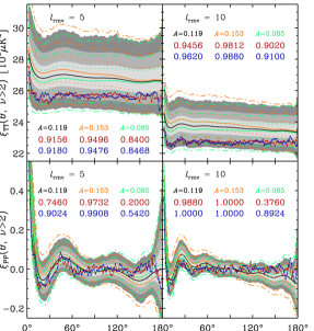
Figure 1: The full-sky TT (upper panel) and PP (lower panel) correlation functions (180 bins) of local extrema for $\nu>2$ with $\ell_{\rm rmv}=5$ and 10. The red (blue) lined-dots correspond to the correlation function of local maxima (minima) observed in the WMAP V-band data. The light, middle and dark gray shaded bands show, respectively, the 68.26%, 95.44%, 99.74% confidence regions determined from 2500 MC simulations for dmf of $\rm V^{A=0.119}_{\textbf{{p}}=(224^{\circ},-22^{\circ})}$, and the black solid line shows the median, as well as the confidence regions and the median of $+/-1\sigma$ variation of the dmf amplitude shown by orange/green lines (solid for the medians, dotted, dashed and dot-dashed for boundaries of 68.26%, 95.44% and 99.74% confidence regions, respectively). The probabilities of finding a simulation with corresponding $\chi^{2}$ values lower than the observed ones are marked for both maxima (red) and minima (blue).

The two-point results are more revealing. The full-sky results for both $\xi_{\rm TT}(\nu\!<\!\infty)$ and $\xi_{\rm PP}(\nu\!<\!\infty)$ show few deviations from the non-modulated model and so cannot change the previous conclusions for these cases. For $\xi_{\rm TT}(\nu\!>\!2)$, especially with $\ell_{\rm rmv}=5$ and 10 as shown by the upper panel of Figure 1, the $\chi^{2}$-frequencies of observation are increasing as the amplitude of the applied dmf increases. The relative spacing of the medians and the confidence interval bands shows that such a shifting is scale-dependent, decreasing on larger scales and providing evidence that the observation does not favor a full-sky dmf since, as found previously, the shape of the observed $\xi_{\rm TT}(\nu\!>\!2)$ fits the non-modulated median quite well.

We then investigate $\xi_{\rm PP}(\nu\!>\!2)$ to find the impact on the spatial distribution of the local extrema by the dmf. The lower panel of Figure 1 indicates that for realisations with the first 5 or 10 multipoles subtracted, the local extrema tend to be more clustered on scales less than $90^{\circ}$ while more anti-clustered on larger scales, and this effect becomes more pronounced for a stronger dmf amplitude. However, the full-sky $\xi_{\rm PP}(\nu\!>\!2)$ medians in the equivalent unmodulated cases fit the observations quite well, and simply oscillate about the zero level on scales larger than $90^{\circ}$ indicating an approximately uniform spatial distribution of local extrema with $\nu\!>\!2$. Again, the empirical properties of the dmf are not favoured by observations.

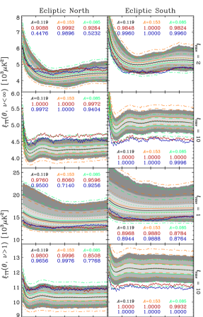
Figure 2: The Ecliptic North and South $\xi_{\rm TT}(\nu\!<\!\infty)$ (the upper two panels for $\ell_{\rm rmv}=2$ and 10) and $\xi_{\rm TT}(\nu\!>\!1)$ (the lower two panels for $\ell_{\rm rmv}=1$ and 10) with dmf $\rm V^{A=0.119\pm 0.034}_{\textbf{{p}}=(224^{\circ},-22^{\circ})}$. The nomenclature of the lined-dots, bands, lines and numbers follows the same style as Figure 1.

The hemispherical results of $\xi_{\rm PP}$ show similar behavior to the full-sky ones on scales less than $90^{\circ}$ and so we focus on $\xi_{\rm TT}$ results for the Ecliptic hemispheres here. As discussed in our previous work, on the GN and EN hemispheres with $\ell_{\rm rmv}=1$ and 2, the observed $\xi_{\rm TT}(\nu\!<\!\infty)$ is suppressed on scales less than $20^{\circ}$ and $\xi_{\rm TT}(\nu\!>\!1,\!2)$ are disfavoured at the $3\sigma$-level in comparison with the Gaussian isotropic model. In contrast, the results for the GS and ES, as well as for correlation functions with $\ell_{\rm rmv}=5$ and 10 over a variety of sky-coverages, show good consistency with the predicted medians. The results presented in Figure 2 here indicate an offset in the expected confidence regions between the north and south, and the discrepancy is enhanced with an increasing dmf amplitude. Considering the profile of the dmf, the model practically attempts to solve the suppression problem on the northern hemispheres by imposing an effective north-south amplitude asymmetry that potentially improves the fit in that part of the sky. On scales less than $15^{\circ}$, the median of $\xi_{\rm TT}(\nu\!<\!\infty)$ with $\ell_{\rm rmv}=2$ on EN does match the observations well. However, the model behaves poorly on the ES – the observations lie below the lower $3\sigma$-level for $\nu\!<\!\infty$ and below the $2\sigma$-level for $\nu\!>\!1$. Moreover, after subtracting the first 5 or 10 multipoles, the north-south asymmetry is increased so far that the model cannot fit the observations, as quantified by the $\chi^{2}$-frequencies and consistent with the behaviour of the one-point statistics. A simple interpretation of these results would be that the profile of the dmf is incorrect, and that the amplitude of the effect may also be a function of $\ell$.

3.2 ACW model results

Generally speaking, the local extrema results in the ACW scenario show few differences from the corresponding isotropic results in Hou, Banday & Górski (2009). For the northern hemispheres, the observed variances are still rejected at 95% confidence level for $\ell_{\rm rmv}=1$ and 2, while other one-point statistics are quite consistent with the model expectations, as judged by the hypothesis tests. Improvements in consistency occur again for $\ell_{\rm rmv}=5$ and 10. Nevertheless, we further investigate the variance results on the full-sky, GN and EN as a function of $g_{*}$ (Figure 3), and more sophisticated acceptance/rejection boundaries are applied by setting different significance levels – $\alpha=0.050$, 0.025 and 0.010.

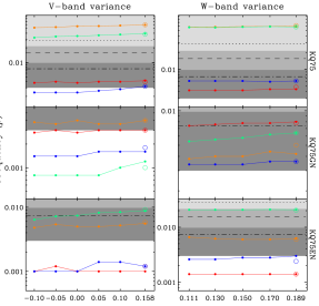
Figure 3: The frequencies ($p$) for which the local extrema variances of 5000 ACW simulations fall below the WMAP5 V and W-band observations as a function of $g_{*}$. Results are shown for the the full-sky (upper panel), GN (middle) and EN (lower). The red (blue) dots and lines correspond to the maxima (minima) frequencies for $\ell_{\rm rmv}=1$, whilst the orange (green) values correspond to $\ell_{\rm rmv}=2$. The centres of the coloured circles correspond to the cases summarised in the last row of Table 2. Note that the red and blue circle in the lower-left panel overlap. The light, middle and dark grey-shaded bands fix the rejection regions in our two-sided hypothesis test with confidence level 95.0%, 97.5% and 99.0%, respectively, with the Type I error $\beta\equiv\alpha$. The dotted, dashed and dot-dashed lines fix the lower-limit of the acceptance regions with $\alpha=0.05$, 0.025 and 0.01, respectively, with the Type II error $\gamma\equiv\alpha$. A logarithmic coordinate is applied to the vertical axis to clearly show the acceptance/rejection boundaries.

The $p$-values for the full-sky V-band variances exhibit an increasing trend $g_{*}$ value (note that we have added our previous results for isotropic ($g_{*}=0.00$) simulations to the plot), although such a trend is not apparent for the W-band. The frequencies of the $\ell_{\rm rmv}=1$ minima (blue lines and dots in Figure 3) are asserted to be rejected at 99% C.L., while not being 99% rejected (but still not accepted at the same level) when $g_{*}$ increases to its 95% confidence upper limit, 0.158. Despite the apparent increasing trend in the V-band, the $\ell_{\rm rmv}=1$ maxima (red lines and dots) variances are still not accepted at 99% C.L., while results of $\ell_{\rm rmv}=2$ are accepted within 95% C.L., also showing the increasing trend. This indicates that the ACW isotropy violation model shows mild improvement in the agreement with observations of the full-sky extrema variances. Nevertheless, the improvement for the cases with $\ell_{\rm rmv}=1$ is inadequate to be accepted by the hypothesis test even at a significance level of 0.01. The results on GN and EN show similar features. The observed maxima variance on the W-band GN hemisphere increases with $g_{*}$ and is accepted at 0.01 significance level, as are the minima on the V-band EN hemisphere with $\ell_{\rm rmv}=2$. There are no other acceptance/rejection changes as a function of $g_{*}$.

It is a natural concern as to the extent to which an incorrectly adopted value for the preferred direction can affect results. Groeneboom & Eriksen (2009) found a $20^{\circ}$ deviation of the best-fitting $\textbf{{n}}^{\prime}$ between V and W-band. Therefore, we assume that such a deviation represents the typical estimation error on the preferred direction and test its impact by, for example, fixing the maximum $g_{*}$ estimated from the W-band but setting $\textbf{{n}}^{\prime}$ as that estimated from the V-band, as summarised in the last row of Table 2. However, as indicated by the coloured circles in Figure 3, no qualitative change is seen.

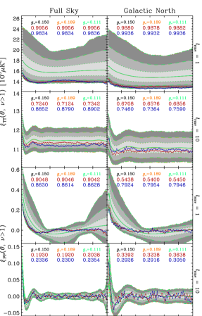
Figure 4: The full-sky and Galactic North $\xi_{\rm TT}(\nu\!>1)$ (the upper two panels for $\ell_{\rm rmv}=1$ and 10) and $\xi_{\rm PP}(\nu\!>\!1)$ (the lower two panels for $\ell_{\rm rmv}=1$ and 10) with 5000 ACW simulations on W-band, $g_{*}=0.150\pm 0.039$, $\textbf{{n}}^{\prime}=(130^{\circ},10^{\circ})$. The nomenclature of the lined-dots, bands, lines and numbers follows the same style as Figure 1. Note that the medians and the boundaries of confidence region are more or less overlapped.

Some of the two-point correlation results of ACW simulations are highlighted in Figure 4. Even though the $\chi^{2}$-frequencies decrease for larger $g_{*}$ values, the $3\sigma$-level suppression of $\xi_{\rm TT}(\nu\!>1,\ell_{\rm rmv}=1,2)$ on the full-sky, GN and EN is still robust for the W-band, and the ACW model does not cause the $\chi^{2}$-frequencies to improve sufficiently until the first 5 or 10 multipoles are subtracted. The confidence regions deviate little as $g_{*}$ varies within its 95% estimation error, constraining the observations almost at the same level as the isotropic model, for both $\xi_{\rm TT}$ and $\xi_{\rm PP}$. It is thus convincingly indicated that the ACW model alone is unable to reconcile the local extrema anomalies originally found in the context of an isotropic Gaussian model of CMB fluctuations.

4 CONCLUSIONS

In this paper, the statistical properties of local temperature extrema in the 5-year WMAP data have been compared with two models that break rotational invariance – dipole modulation and the ACW model. Such a comparison was motivated by the fact that our previous analysis of local extrema statistics (Hou, Banday & Górski, 2009) demonstrated an unlikely hemispherical asymmetry in the GN and EN as a consequence of an extremely low-variance compared to the expectations of a Gaussian isotropic scenario. Moreover, the 5-year WMAP data indicate significant detections of these models on the basis of power spectrum analyses.

We employ Gaussian MC simulations encoding the features of these two models to establish the statistical basis for testing whether the breaking of rotational invariance by the models can afford a satisfactory explanation of local extrema anomalies. As in previous work, both one and two-point statistics, as well as their dependence on large angular-scale modes have been studied. Both models are parameterised by a set of amplitudes and preferred directions as established by independent Bayesian analyses in Hoftuft et al. (2009) and Groeneboom & Eriksen (2009). Our analysis has been carried out by sampling the former within their 95% confidence intervals, whilst imposing the fixed preferred direction found for each band, since the latter are estimated to be robust for each model. The V and W-band data are considered here.

In fact, the local extrema studies based on one and two-point statistics indicate that neither model provides a satisfactory solution to observed properties. In particular, the ACW model is probably the least interesting in this context – both the one-point analysis and two-point studies show similar features to the isotropic results, including their $\ell$-dependence. The dipolar modulation field, however, may itself be constrained by our analysis.

Results determined from division of the data into hemispheres implies that a dmf with significant amplitude may suppress the observed variance anomalies. In particular, the $\ell_{\rm rmv}=2$ values on EN and ES hemispheres indicates consistency of the data with the model. However, after subtraction of the first 10 multipoles, new problems arise in the southern hemispheres, where the observed variance of local extrema is now much lower than the model prediction. This is suggestive that the dmf may not have the correct profile over the full-sky in order to reconcile the variance properties of the observed local extrema with the Gaussian anisotropic simulations, and that the amplitude of the effect may also be a function of $\ell$. Moreover, the observed mean statistics, which showed few anomalies when compared to the Gaussian isotropic model, are not consistent and contradict the variance results by requiring a weaker amplitude.

Our analysis indicates that neither a simple dipole modulated field model nor a rotational-invariance breaking model can satisfactorily explain the local extrema anomalies present in the WMAP data. On the one side, the rotational-invariance model affects the large-scale temperature amplitudes too little to significantly affect the local extrema statistics. On the other side, a modulation type model needs a more elaborate spatial structure than a simple dipole to fully fit the data. These issues remain interesting for further investigation.

References

- Ackerman, Carroll & Wise (2007) Ackerman L., Carroll S. M., Wise M. B., 2007, PRD, 75, 083502
- Barreiro et al. (1997) Barreiro R. B., Sanz J. L., Martínez-González E., Cayón L., Silk J., 1997, ApJ, 478, 1
- Bennett et al. (2003) Bennett C. L., et al., 2003, ApJS, 148, 1
- Bond & Efstathiou (1987) Bond J. R., Efstathiou G., 1987, MNRAS, 226, 655
- Eriksen et al. (2007) Eriksen H. K., Banday A. J., Górski K. M., Hansen H. K., Lilje P. B., 2007, ApJ, 660, L81
- Eriksen et al. (2004) Eriksen H. K., Hansen F. K., Banday A. J., Górski K. M., Lilje P. B., 2004, ApJ, 605, 14
- Eriksen et al. (2005) Eriksen H. K., Banday A. J., Górski K. M., Lilje P. B., 2005, ApJ, 622, 58
- Górski et al. (2005) Górski K. M., Hivon E., Banday A. J., Wandelt B. D., Hansen F. K., Reinecke M., Bartelmann M., 2005, ApJ, 622, 759
- Gordon et al. (2005) Gordon C., Hu W., Huterer D., Crawford T., 2005, PRD, 72, 103002
- Groeneboom & Eriksen (2009) Groeneboom N. E., Eriksen H. K., 2009, ApJ, 690, 1807
- Hamilton (1993) Hamilton A. J., 1993, ApJ, 417, 19
- Hansen, Banday & Górski (2004) Hansen F. K., Banday A. J., Górski K. M., 2004, MNRAS, 354, 641
- Hansen et al. (2008) Hansen F. K., Banday A. J., Górski K. M., Eriksen H. K., Lilje P. B., 2008, preprint (arXiv:0812.3795)
- Heavens & Sheth (1999) Heavens A. F., Sheth R. K., 1999, MNRAS, 310, 1062
- Heavens & Gupta (2001) Heavens A. F., Gupta S., 2001, MNRAS, 324, 960
- Hinshaw et al. (2007) Hinshaw G., et al., 2007, ApJS, 170, 288
- Hoftuft et al. (2009) Hoftuft J., Eriksen H. K., Banday A. J., Górski K. M., Hansen H. K., Lilje P. B., 2009, ApJ, 699, 985
- Hou, Banday & Górski (2009) Hou Z., Banday A. J., Górski K. M., 2009, MNRAS, 396, 1273
- Kogut et al. (1995) Kogut A., Banday A. J., Bennett C. L., Hinshaw G., Lubin P. M, Smoot G. F., 1995, ApJ, 439, L29
- Kogut et al. (1996) Kogut A., Banday A. J., Bennett C. L., Górski K. M., Hinshaw G., Smoot G. F., Wright E. L., 1996, ApJ, 464, L29
- Komatsu et al. (2009) Komatsu E., et al., 2009, ApJS, 180, 330
- Larson & Wandelt (2004) Larson D. L., Wandelt B. D., 2004, ApJ, 613, L85
- Larson & Wandelt (2005) Larson D. L., Wandelt B. D., 2005, preprint (arXiv:astro-ph/0505046)
- Lewis, Challinor & Lasenby (2000) Lewis A., Challinor A., Lasenby A., 2000, ApJ, 538, 473
- Nolta et al. (2009) Nolta M. R., et al, 2009, ApJS, 180, 296
- Park C-G (2004) Park, C-G, 2004, MNRAS, 349, 313
- Tojeiro et al. (2006) Tojeiro R., Castro P. G., Heavens A. F., Gupta S., 2006, MNRAS, 365, 265
- Vittorio & Juszkiewicz (1987) Vittorio N., Juszkiewicz R., 1987, ApJ, 314, L29
- Wandelt, Hivon & Górski (1998) Wandelt B. D., Hivon E., Górski K. M., 1998, preprint (arXiv:astro-ph/9803317), to appear in ‘Fundemental Parameters in Cosmology’, proceedings of the 33rd Rencontres de Moriond, edited by Tran Thanh Van, 237–240 (1999)
- Wehus et al. (2009) Wehus I. K., Ackerman L., Eriksen H. K., Groeneboom N. E., 2009, preprint (arXiv:0904.3998)