A Scalable VLSI Architecture for Soft-Input Soft-Output Depth-First Sphere Decoding^∗

Abstract

Multiple-input multiple-output (MIMO) wireless transmission imposes huge challenges on the design of efficient hardware architectures for iterative receivers. A major challenge is soft-input soft-output (SISO) MIMO demapping, often approached by sphere decoding (SD). In this paper, we introduce the—to our best knowledge—first VLSI architecture for SISO SD applying a single tree-search approach. Compared with a soft-output-only base architecture similar to the one proposed by Studer et al. in IEEE J-SAC 2008, the architectural modifications for soft input still allow a one-node-per-cycle execution. For a 4$\times$4 16-QAM system, the area increases by 57 % and the operating frequency degrades by 34 % only.

Manuscript received October 26, 2009; revised April 5, 2010. This work has been supported by the UMIC (Ultra High-Speed Mobile Information and Communication) Research Centre at the RWTH-Aachen University.

The authors are with the Institute for Integrated Signal Processing Systems, RWTH-Aachen University, D-52056 Aachen, Germany (email: {witte,borlenghi,ascheid,leupers,meyr}@iss.rwth-aachen.de).

I Introduction

Multiple-input multiple-output (MIMO) wireless transmissions utilizing spatial multiplexing achieve an increased spectral efficiency compared with single-antenna systems. This improvement comes at the cost of an increased signal-demapping complexity, which becomes particularly critical for iterative receivers [1]. Recent developments of soft-input soft-output (SISO) MIMO-demapping algorithms reduced this complexity significantly. Prominent demapping algorithms are k-best and list-based approaches [2, 3], Markov chain Monte Carlo algorithms (MCMC) [4] and single tree-search (STS) sphere decoders (SD) [5]. The STS approach is often preferred since it guarantees max-log maximum a posteriori (MAP) optimality.

Efficient VLSI implementations have been proposed for soft-output-only STS SDs [6, 7] exploiting geometric properties of QAM constellations. These geometric relations help determining a search order, defined as enumeration, leading to a fast average tree-search convergence. The SISO STS complexity has been prohibitive for VLSI implementations so far, because geometric relations are not applicable directly. Recent improvements of soft-input enumeration strategies moved SISO STS SD closer to VLSI architectures [8].

Contributions: In this paper, we introduce the—to our best knowledge—first VLSI architecture for SISO STS SD. It is based on a soft-output-only architecture following the one-node-per-cycle (ONPC) paradigm used by [6]. The SISO modifications are modular enough to be applied to other existing STS SD architectures and still allow ONPC execution. Compared with a soft-output-only architecture, the area increases by 57 % and the clock frequency degrades by 34 % for a $4\times 4$ 16-QAM system. Thus, this architecture enables STS-based iterative wireless MIMO receivers.

The paper is organized as follows: Section II sums up the basics of SISO STS SD, extended by the soft-input enumeration strategy in Section III. Section IV describes important implementation aspects of the scalable VLSI architecture. In Section V the parameter design space of the SISO STS architecture as well as area, timing and throughput are discussed.

II Single Tree-Search Soft-Input Sphere Decoding

A spatial-multiplexing MIMO scheme with $M_{\textrm{T}}$ transmit and $M_{\textrm{R}}\geq M_{\textrm{T}}$ receive antennas is assumed [1]. Each transmit antenna sends one of the $2^{Q}$ complex elements of the symbol set $\mathcal{O}$ defined by the modulation alphabet, which is assumed to be the same for every antenna. Each vector $\textbf{s}=\left[s_{1},...,s_{M_{\textrm{T}}}\right]^{T}\in\mathcal{O}^{M_{\textrm{T}}}$ results from mapping $M_{\textrm{T}}{}Q$ bits $x_{i,b}\in\{+1,-1\}$ to an element of $\mathcal{O}^{M_{\textrm{T}}}$, with $i$ being the antenna index and $b$ the bit index for one scalar symbol $s_{i}$.

The received symbol vector $\textbf{y}\in\mathbb{C}^{M_{\textrm{R}}}$ is given by $\textbf{y}~{}=~{}\textbf{H}\textbf{s}~{}+~{}\textbf{n}$, where $\textbf{H}\in\mathbb{C}^{M_{\textrm{R}}\times M_{\textrm{T}}}$ is the channel matrix and $\textbf{n}\in\mathbb{C}^{M_{\textrm{R}}}$ is a white circular Gaussian noise vector with variance $N_{\textrm{0}}$ per element. For tree-search SD, H is typically QR-decomposed (QRD) with $\textbf{H}=\textbf{Q}\textbf{R}$, $\textbf{Q}\in\mathbb{C}^{M_{\textrm{R}}\times M_{\textrm{T}}}$ and $\textbf{Q}^{H}\textbf{Q}=\textbf{I}$ and $\textbf{R}\in\mathbb{C}^{M_{\textrm{T}}\times M_{\textrm{T}}}$ being an upper triangular matrix [1, 5]. With $\tilde{\textbf{y}}=\textbf{Q}^{H}\textbf{y}$ and $\tilde{\textbf{n}}=\textbf{Q}^{H}\textbf{n}$, this results in

$$\tilde{\textbf{y}}=\textbf{R}\textbf{s}+\tilde{\textbf{n}}\quad.$$ (1)

According to [5], the triangular matrix R in equation (1) allows to formulate the SISO max-log MAP MIMO detection problem as STS within a $2^{Q}$-ary complete tree. The tree levels correspond to the $M_{\textrm{T}}$ antennas, each node ${s}_{i}\in\mathcal{O}$ on tree level $i$ is a received symbol candidate, with $s_{1}$ being a leaf node. An exhaustive search in such a tree leads to a worst-case run-time complexity of $O(2^{QM_{\textrm{T}}})$. As formalized in equations (2) to (4), metric increments $\mathcal{M}_{\textrm{C}}({s}_{i})$ for channel-based and $\mathcal{M}_{\textrm{A}}({s}_{i})$ for a priori-based information are summed up to a total increment $\mathcal{M}_{\textrm{P}}({s}_{i})$. $\textrm{P}[{s}_{i}]$ is the symbol probability computed from the a priori log-likelihood ratios (LLRs) $L^{\textrm{A}}_{i,b}$.

$$\mathcal{M}_{\textrm{A}}({s}_{i}) = -\log\textrm{P}[{s}_{i}]$$ (2)

$$\mathcal{M}_{\textrm{C}}({s}_{i}) = \frac{1}{N_{\textrm{0}}}|\tilde{{y}_{i}}-\sum_{j=i}^{M_{\textrm{T}}}{R}_{{i},{j}}{s}_{j}|^{2}$$ (3)

$$\mathcal{M}_{\textrm{P}}({s}_{i}) = \mathcal{M}_{\textrm{C}}({s}_{i})+\mathcal{M}_{\textrm{A}}({s}_{i})$$ (4)

The sum of metric increments along a path from the root to node ${s}_{i}$ yields the partial metric $\mathcal{M}_{\textrm{P}}(\textbf{s}^{(i)})$ for a partial symbol vector $\textbf{s}^{(i)}=[s_{i},...,s_{M_{\textrm{T}}}]^{T}$:

$$\mathcal{M}_{\textrm{P}}(\textbf{s}^{(i)}) = \sum_{j=i}^{M_{\textrm{T}}}\mathcal{M}_{\textrm{P}}({s}_{j})$$ (5)

During a STS, the MAP solution $\textbf{s}^{\textrm{MAP}}$, its bits $x_{i,b}^{\textrm{MAP}}$ and metric $\lambda^{\textrm{MAP}}\!=\!\mathcal{M}_{\textrm{P}}(\textbf{s}^{\textrm{MAP}})$ and extrinsic counter-hypothesis metrics $\Lambda^{\overline{\textrm{MAP}}}_{i,b}$ are computed by successively improving the current metrics $\lambda^{\textrm{MAP},\textrm{cur}}$ and $\Lambda^{\overline{\textrm{MAP}},\textrm{cur}}_{i,b}$. $L^{\textrm{E}}_{i,b}$ are extrinsic LLRs with

$$\textbf{s}^{\textrm{MAP}} = \underset{\textbf{s}\in\mathcal{O}^{M_{\textrm{T}}}}{\arg\min}\left\{\mathcal{M}_{\textrm{P}}(\textbf{s})\right\}$$

$$\Lambda^{\overline{\textrm{MAP}}}_{i,b} = \underset{\textbf{s}\in\mathcal{O}^{M_{\textrm{T}}}\wedge x_{i,b}\neq x_{i,b}^{\textrm{MAP}}}{\min}\left\{\mathcal{M}_{\textrm{P}}(\textbf{s})\right\}-L^{\textrm{A}}_{i,b}x_{i,b}^{\textrm{MAP}}$$

$$L^{\textrm{E}}_{i,b} = \left(\Lambda^{\overline{\textrm{MAP}}}_{i,b}-\lambda^{\textrm{MAP}}\right)x_{i,b}^{\textrm{MAP}}\quad.$$

These metric computations dominate the detection complexity. For a depth-first tree search, the pruning of sub-trees lying outside a hypersphere with a radius not improving $\lambda^{\overline{\textrm{MAP}},\textrm{cur}}_{i,b}\!=\!\Lambda^{\overline{\textrm{MAP}},\textrm{cur}}_{i,b}\!+\!L^{\textrm{A}}_{i,b}x_{i,b}^{\textrm{MAP}}$ provides a heuristic for complexity reduction which is sensitive to the visiting order $[{s}_{i}^{(1)},...,{s}_{i}^{(|\mathcal{O}|)}]$. A Schnorr-Euchner (SE) order [9] provides a very fast search convergence by the following pruning criteria [6], typically defining the pruning metrics $\mathcal{M}_{\textrm{prn},j}^{\textrm{down}}\!:=\!\mathcal{M}_{\textrm{prn},j}^{\textrm{sibl.}}\!:=\!\mathcal{M}_{\textrm{P}}(\textbf{s}^{(j)})$:

$$\mathcal{M}_{\textrm{prn},j}^{\textrm{down}}\geq\max{\left\{\left.\lambda^{\overline{\textrm{MAP}},\textrm{cur}}_{i,b}\right|i<j\vee x_{i,b}\neq x_{i,b}^{\textrm{MAP},\textrm{cur}},\forall b\right\}}$$ (6)

$$\mathcal{M}_{\textrm{prn},j}^{\textrm{sibl.}}\geq\max{\left\{\left.\lambda^{\overline{\textrm{MAP}},\textrm{cur}}_{i,b}\right|i\leq j\vee x_{i,b}\neq x_{i,b}^{\textrm{MAP},\textrm{cur}},\forall b\right\}}$$ (7)

If inequality (6) holds, the current node and its sub-tree are pruned, otherwise a step down is performed in the tree. If inequality (7) holds, the enumeration on level $j$ stops, otherwise the sibling of the current node is enumerated. The arguments of the $\max{}$ operators in (6) and (7) are the sets $\mathcal{A}$ and $\mathcal{B}$ respectively in [6]. We define an examined node (as used in [6] and [7]) as a node ${s}_{j}$ that has been checked against at least one pruning criterion, leading to the complexity measure number of examined nodes per detected symbol vector $N_{\textrm{en}}$.

If a leaf node with $\mathcal{M}_{\textrm{P}}(\textbf{s})\geq\lambda^{\textrm{MAP},\textrm{cur}}$ is not pruned by inequalities (6) or (7), the values $\{\Lambda^{\overline{\textrm{MAP}},\textrm{cur}}_{i,b}|x_{i,b}\neq x_{i,b}^{\textrm{MAP},\textrm{cur}}\}$ need to be updated by $\min{\{\Lambda^{\overline{\textrm{MAP}},\textrm{cur}}_{i,b},\mathcal{M}_{\textrm{P}}(\textbf{s})-L^{\textrm{A}}_{i,b}x_{i,b}^{\textrm{MAP},\textrm{cur}}\}}$. Otherwise, if $\mathcal{M}_{\textrm{P}}(\textbf{s})<\lambda^{\textrm{MAP},\textrm{cur}}$, the current leaf becomes the new MAP solution and the extrinsic counter-hypothesis metrics $\{\Lambda^{\overline{\textrm{MAP}},\textrm{cur}}_{i,b}|x_{i,b}^{\textrm{MAP},\textrm{old}}\neq x_{i,b}^{\textrm{MAP},\textrm{cur}}\}$ are updated by $\min{\{\Lambda^{\overline{\textrm{MAP}},\textrm{cur}}_{i,b},\lambda^{\textrm{MAP},\textrm{old}}-L^{\textrm{A}}_{i,b}x_{i,b}^{\textrm{MAP},\textrm{cur}}\}}$.

Many methods exist to reduce $N_{\textrm{en}}$, like sorted QRD (SQRD) [10] and extrinsic LLR clipping [5]. The latter one limits the allowed range for $L^{\textrm{E}}_{i,b}$ to $|L^{\textrm{E}}_{i,b,\textrm{clipped}}|\leq L^{\textrm{E}}_{\textrm{max}}$, which leads to clipped extrinsic metrics $\Lambda^{\overline{\textrm{MAP}}}_{i,b,\textrm{clipped}}$:

$$\Lambda^{\overline{\textrm{MAP}}}_{i,b,\textrm{clipped}}\!=\!\max\left\{\lambda^{\textrm{MAP}}\!-\!L^{\textrm{E}}_{\textrm{max}},\min\left\{\lambda^{\textrm{MAP}}\!+\!L^{\textrm{E}}_{\textrm{max}},\Lambda^{\overline{\textrm{MAP}}}_{i,b}\right\}\right\}$$ (8)

Please note that equation (8) is stricter than the $\min\{\}$ function used in [5] where a post-processing step is used to guarantee $|L^{\textrm{E}}_{i,b,\textrm{clipped}}|~{}\leq~{}L^{\textrm{E}}_{\textrm{max}}$ for proper channel decoding. In [5], this saves 50 % of the comparisons required for clipping. Experiments indicate that $\mathbb{E}[N_{\textrm{en}}]$ differs only marginally between the two clipping methods. Moreover, radius tightening further reduces $N_{\textrm{en}}$. A hardware-friendly approximation of $\mathcal{M}_{\textrm{A}}({s}_{i})$ for statistically independent symbols, including tightening and still guaranteeing max-log-optimal a posteriori LLRs, has been proposed in [5] (with unipolar bits $d_{i,b}\!=\!\frac{1}{2}(1-x_{i,b}\cdot\mathrm{sign}(L^{\textrm{A}}_{i,b}))$):

$$\mathcal{M}_{\textrm{A}}({s}_{i})=-\log\textrm{P}[{s}_{i}]\approx\sum_{b=1}^{Q}\begin{cases}|L^{\textrm{A}}_{i,b}|,&d_{i,b}=1\\ 0,&\textrm{otherwise}\end{cases}$$ (9)

III The Hybrid-Enumeration Algorithm

A major issue of SD algorithms is the enumeration process, namely the determination of the SE order $[{s}_{i}^{(1)},...,{s}_{i}^{(|\mathcal{O}|)}]$ on a level $i$ with ${s}_{i}^{(k)}$ representing the $k^{\textrm{th}}$ candidate for node ${s}_{i}$, in ascending order of $\mathcal{M}_{\textrm{P}}$. A straightforward implementation by computing and fully sorting the set $\{\mathcal{M}_{\textrm{P}}({s}_{i}^{(k)})\}$ is very expensive and inefficient. For the soft-output-only case, the geometric properties of the QAM constellation can be exploited to avoid full sorting and thus save most of the computations, as proposed in [6, 11, 7]. However, in iterative receivers these optimizations are not usable directly because the geometry-based order is scrambled by the a priori information. A viable approach towards efficient soft-input enumeration is given by the hybrid-enumeration algorithm presented in [8]. Its basic idea is to split the enumeration of $\{\mathcal{M}_{\textrm{P}}({s}_{i}^{(k)})\}$ into two concurrent enumerations of $\{\mathcal{M}_{\textrm{C}}({s}_{i}^{(k)})\}$ and $\{\mathcal{M}_{\textrm{A}}({s}_{i}^{(k)})\}$.

On the one hand, the enumeration of $\{\mathcal{M}_{\textrm{C}}({s}_{i}^{(k)})\}$ is the same as in the soft-output-only case, thus allowing to reuse any of the related aforementioned efficient methods, even in later iterations. On the other hand, the enumeration of $\{\mathcal{M}_{\textrm{A}}({s}_{i}^{(k)})\}$ is efficient as well since the linear sorting of the symbol set $\mathcal{O}$ needs to be performed independently only once per antenna.

According to [8], the channel- and a priori-based enumerations independently select candidate symbols ${s}_{\textrm{C},i}^{(k)}$ and ${s}_{\textrm{A},i}^{(k)}$ at each step $k$. The hybrid enumeration simply selects the candidate with the lower metric $\mathcal{M}_{\textrm{P}}$ between these two.

\psfrag{Ma}[Bc][Bc][1][0]{\footnotesize$\mathcal{M}_{\textrm{A}}$}\psfrag{Mc}[Br][Br][1][0]{\footnotesize$\mathcal{M}_{\textrm{C}}$}\psfrag{step}[Bc][Bc][1][0]{\scriptsize step $k$}\psfrag{k1}[Bc][Bc][1][0]{\scriptsize$1$}\psfrag{k2}[Bc][Bc][1][0]{\scriptsize$2$}\psfrag{k3}[Bc][Bc][1][0]{\scriptsize$3$}\psfrag{k4}[Bc][Bc][1][0]{\scriptsize$4$}\psfrag{CMa}[Bc][Bc][1][0]{\scriptsize$\mathcal{M}_{\textrm{P}}({s}_{\textrm{A},i}^{(k)})$}\psfrag{ma1}[Bc][Bc][1][0]{\scriptsize$\mathcal{M}_{\textrm{P}}(O^{(2)})$}\psfrag{ma2}[Bc][Bc][1][0]{\scriptsize$\mathcal{M}_{\textrm{P}}(O^{(1)})$}\psfrag{ma3}[Bc][Bc][1][0]{\scriptsize$\mathcal{M}_{\textrm{P}}(O^{(4)})$}\psfrag{ma4}[Bc][Bc][1][0]{\scriptsize{\color[rgb]{0.3,0.3,0.3}$\mathcal{M}_{\textrm{P}}(O^{(4)})$}}\psfrag{ma5}[Bc][Bc][1][0]{\scriptsize{\color[rgb]{0.3,0.3,0.3}$\mathcal{M}_{\textrm{P}}(O^{(4)})$}}\psfrag{ma6}[Bc][Bc][1][0]{\scriptsize$\mathcal{M}_{\textrm{P}}(O^{(4)})$}\psfrag{r1}[Bc][Bc][1][0]{\scriptsize$<$}\psfrag{r2}[Bc][Bc][1][0]{\scriptsize$<$}\psfrag{r3}[Bc][Bc][1][0]{\scriptsize$>$}\psfrag{r4}[Bc][Bc][1][0]{\scriptsize{\color[rgb]{0.3,0.3,0.3}$>$}}\psfrag{r5}[Bc][Bc][1][0]{\scriptsize{\color[rgb]{0.3,0.3,0.3}$>$}}\psfrag{r6}[Bc][Bc][1][0]{\scriptsize$=$}\psfrag{CMc}[Bc][Bc][1][0]{\scriptsize$\mathcal{M}_{\textrm{P}}({s}_{\textrm{C},i}^{(k)})$}\psfrag{mc1}[Bc][Bc][1][0]{\scriptsize$\mathcal{M}_{\textrm{P}}(O^{(3)})$}\psfrag{mc2}[Bc][Bc][1][0]{\scriptsize$\mathcal{M}_{\textrm{P}}(O^{(3)})$}\psfrag{mc3}[Bc][Bc][1][0]{\scriptsize$\mathcal{M}_{\textrm{P}}(O^{(3)})$}\psfrag{mc4}[Bc][Bc][1][0]{\scriptsize{\color[rgb]{0.3,0.3,0.3}$\mathcal{M}_{\textrm{P}}(O^{(1)})$}}\psfrag{mc5}[Bc][Bc][1][0]{\scriptsize{\color[rgb]{0.3,0.3,0.3}$\mathcal{M}_{\textrm{P}}(O^{(2)})$}}\psfrag{mc6}[Bc][Bc][1][0]{\scriptsize$\mathcal{M}_{\textrm{P}}(O^{(4)})$}\psfrag{E}[Bc][Bc][1][0]{\scriptsize${s}_{i}^{(k)}$}\psfrag{n1}[Bc][Bc][1][0]{\scriptsize$O^{(2)}$}\psfrag{n2}[Bc][Bc][1][0]{\scriptsize$O^{(1)}$}\psfrag{n3}[Bc][Bc][1][0]{\scriptsize$O^{(3)}$}\psfrag{n4}[Bc][Bc][1][0]{\scriptsize{\color[rgb]{0.3,0.3,0.3} \emph{skipped}} }\psfrag{n5}[Bc][Bc][1][0]{\scriptsize{\color[rgb]{0.3,0.3,0.3} \emph{skipped}} }\psfrag{n6}[Bc][Bc][1][0]{\scriptsize$O^{(4)}$}\psfrag{Mp1}[Bc][Bc][1][0]{\scriptsize$\mathcal{M}_{\textrm{P}}(O^{(1)})$}\psfrag{Mp2}[Bc][Bc][1][0]{\scriptsize$\mathcal{M}_{\textrm{P}}(O^{(2)})$}\psfrag{Mp3}[Bc][Bc][1][0]{\scriptsize$\mathcal{M}_{\textrm{P}}(O^{(3)})$}\psfrag{o1}[cc][cc][1][0]{\tiny$O^{(1)}$}\psfrag{o2}[cc][cc][1][0]{\tiny$O^{(2)}$}\psfrag{o3}[cc][cc][1][0]{\tiny$O^{(3)}$}\psfrag{o4}[cc][cc][1][0]{\tiny$O^{(4)}$}\psfrag{1}[Bc][Bc][1][0]{\scriptsize$k\!=\!1$}\psfrag{2}[Bc][Bc][1][0]{\scriptsize$k\!=\!2$}\psfrag{34}[Bc][Bc][1][0]{\scriptsize$k\!\in\!\{3,\!4\}$}\psfrag{4}[Bc][Bc][1][0]{\scriptsize$k\!=\!4$}\psfrag{123}[Br][Br][1][0]{\scriptsize$k\!\in\!\{1,\!2,\!3\}$}\includegraphics[width=216.81pt]{hybrid-enumeration}

Figure 1: Hybrid-enumeration example, $k^{th}$ symbol in SE order: $O^{(k)}\in\mathcal{O}$.

As visualized in Figure 1, the strict SE order is not preserved, hence the inequality $\mathcal{M}_{\textrm{P}}({s}_{i}^{(k)})\leq\mathcal{M}_{\textrm{P}}({s}_{i}^{(l)}),\forall l>k$ does not hold any more. Thus, a modification of the pruning criteria is needed to avoid the erroneous exclusion of the MAP or counter-hypothesis solutions. For $l>k$, the inequalities $\mathcal{M}_{\textrm{C}}({s}_{\textrm{C},i}^{(k)})\leq\mathcal{M}_{\textrm{C}}({s}_{\textrm{C},i}^{(l)})$ and $\mathcal{M}_{\textrm{A}}({s}_{\textrm{A},i}^{(k)})\leq\mathcal{M}_{\textrm{A}}({s}_{\textrm{A},i}^{(l)})$ lead to $\mathcal{M}_{\textrm{C}}({s}_{\textrm{C},i}^{(k)})+\mathcal{M}_{\textrm{A}}({s}_{\textrm{A},i}^{(k)})\leq\mathcal{M}_{\textrm{P}}({s}_{i}^{(l)})$, providing an alternative lower bound for tree pruning. Thus, in [8] the pruning metric of inequality (7) on the current tree level $i$ is re-defined as

$$\mathcal{M}_{\textrm{prn},i}^{\textrm{sibl.}}:=\mathcal{M}_{\textrm{C}}({s}_{\textrm{C},i}^{(k)})+\mathcal{M}_{\textrm{A}}({s}_{\textrm{A},i}^{(k)})+\mathcal{M}_{\textrm{P}}(\textbf{s}^{(i+1)})\quad.$$ (10)

Compared with the SE order, pruning metric (10) preserves the error-rate performance at the price of a slight increase in $N_{\textrm{en}}$. For a more detailed description and analysis of the hybrid-enumeration algorithm, the reader is referred to [8].

IV A VLSI Architecture for STS Soft-Input Sphere Decoding

In this section, a VLSI architecture for SISO STS SD is introduced. It is derived from a soft-output-only depth-first STS base architecture extended by soft-input processing. The main challenges are discussed that arise from the implementation of efficient soft-input extensions according to the hybrid-enumeration scheme. Further algorithmic optimizations such as LLR correction proposed in [5] are orthogonal to the base architecture and can be implemented on top of it.

IV-A Soft-Output-Only Base Architecture

The soft-output-only base STS architecture, composed of the light gray blocks in Figure 2, follows the ONPC execution principle used by Studer et al. in [6]. Its architectural structure is derived from the observation that the tree search is composed of three basic control-flow steps:

i) Vertical steps (①) down from tree level $i$ to $i-1$ enumerate the first child node ${s}_{i-1}^{(1)}$ of a parent node ${s}_{i}^{(k)}$. This requires a quantization step $\mathcal{Q}$ to find the QAM symbol next to $\tilde{{y}_{i}}$, followed by the computation of $\mathcal{M}_{\textrm{P}}({s}_{i-1}^{(1)})$. The result of $\mathcal{Q}$ is used to initialize the enumeration on the tree level $i-1$ and by the pruning-criteria check for ${s}_{i-1}^{(1)}$.

ii) Horizontal steps (②) on a tree level $i$ enumerate the node ${s}_{i}^{(k+1)}$ after enumerating the node ${s}_{i}^{(k)}$ and its sub-tree. This category also includes steps back from a child node ${s}_{i-1}$ to the next sibling ${s}_{i}^{(k+1)}$ of its parent node ${s}_{i}^{(k)}$.

iii) Pruning-criteria checks (③) for a node ${s}_{i}^{(k)}$ determine if either a vertical step to the child ${s}_{i-1}^{(1)}$, a horizontal step to the sibling ${s}_{i}^{(k+1)}$ or a horizontal step to its parent’s sibling ${s}_{i+1}^{(l+1)}$ has to be performed next. The $\mathcal{M}_{\textrm{P}}$ history (④) unit stores the partial metrics $\mathcal{M}_{\textrm{P}}(\textbf{s}^{(i)})$, recursively implements equation (5) and provides its result to unit ③ for pruning and LLR clipping by equation (8).

In a depth-first SD, the tree-traversal control flow exhibits severe data and control dependencies. In order to achieve a throughput of one examined node per cycle, the base architecture executes the pruning check for node ${s}_{i}^{(k)}$ concurrently with the steps towards ${s}_{i-1}^{(1)}$ and ${s}_{i}^{(k+1)}$ in cycle $n$. If the pruning check selects ${s}_{i-1}^{(1)}$, ${s}_{i}^{(k+1)}$ is saved in a preferred-siblings cache (⑤) for later use during a step up in the tree. Thus, in cycle $n+1$ the availability of a valid node for the next pruning check is guaranteed.

The enumeration unit of the base architecture employs the column-wise zig-zag enumeration strategy (⑥) presented in [11]. Compared with circular PSK-like enumeration [6], the column-wise enumeration allows a much more regular hardware implementation. Furthermore, for 64 QAM and higher modulation orders it requires less comparisons.

Since there is no assumption on the mapping between QAM symbols and bits, two run-time-programmable lookup tables, named mapper $\mathcal{M}$ and demapper $\mathcal{D}$ respectively, are used for the conversion between the symbol and the bit representations.

\psfrag{control}[cc][cc][1][0]{STS Control FSM}\psfrag{InputRegs}[bl][bl][1][0]{$\textbf{R},\tilde{\textbf{y}},\{L^{\textrm{A}}_{i,b}\}$}\psfrag{MatVect}[cc][cc][1][0]{\small$\tilde{{y}_{i}}\!-\!\sum\limits_{j=i+1}^{M_{\textrm{T}}}\!{R}_{{i},{j}}{s}_{j}$}\psfrag{Cache}[bc][bc][1][0]{\small{$M_{\textrm{T}}2^{Q}$ Enumerated Nodes Flags}}\psfrag{colzz}[bc][bc][1][0]{col. zig-zag{}}\psfrag{MC}[bl][bl][1][0]{$\mathcal{M}_{\textrm{C}}$}\psfrag{MA}[bl][bl][1][0]{$\mathcal{M}_{\textrm{A}}$}\psfrag{MA0}[bl][bl][1][0]{$\mathcal{M}_{\textrm{A}}=0$}\psfrag{MP}[bl][bl][1][0]{$\mathcal{M}_{\textrm{P}}$}\psfrag{M}[bc][bc][1][0]{$\mathcal{M}$}\psfrag{D}[bc][bc][1][0]{$\mathcal{D}$}\psfrag{Q}[cc][cc][1][0]{$\mathcal{Q}$}\psfrag{cc}[cc][cc][1][0]{Pruning Criteria, $\{\Lambda^{\overline{\textrm{MAP}}}_{i,b}\},\lambda^{\textrm{MAP}},\{x_{i,b}^{\textrm{MAP}}\}$}\psfrag{LE}[cc][cc][1][0]{$\{L^{\textrm{E}}_{i,b}\}$}\psfrag{CSd}[cc][cc][1][0]{min}\psfrag{CSh}[cc][cc][1][0]{min}\psfrag{min}[cc][cc][1][0]{\small$\mathcal{M}_{\textrm{A,min}}$}\psfrag{min2}[cc][cc][1][0]{\footnotesize$2^{Q}:1$}\psfrag{cmin}[cc][cc][1][0]{\scriptsize{min}}\psfrag{prefch}[cc][cc][1][0]{\scriptsize{$M_{\textrm{T}}-1$ Pref. Siblings}}\psfrag{hist}[cc][cc][1][0]{$\mathcal{M}_{\textrm{P}}$ History}\psfrag{MAs}[cc][cc][1][0]{\small$\{\mathcal{M}_{\textrm{A}}\}_{i}$}\psfrag{c1}[cc][cc][1][0]{\char 172}\psfrag{c2}[cc][cc][1][0]{\char 173}\psfrag{c3}[cc][cc][1][0]{\char 174}\psfrag{c4}[cc][cc][1][0]{\char 176}\psfrag{c5}[cc][cc][1][0]{\char 178}\psfrag{c6}[cc][cc][1][0]{\char 177}\psfrag{c7}[cc][cc][1][0]{\char 179}\psfrag{c8}[cc][cc][1][0]{\char 180}\psfrag{c9}[cc][cc][1][0]{\char 175}\includegraphics[width=216.81pt]{vlsi-architecture}

Figure 2: Block diagram of the proposed soft-input STS SD VLSI architecture. Units added/modified for soft-input are emphasized by dark gray background. Legend: Mapper $\mathcal{M}$, Demapper $\mathcal{D}$, Quantizer $\mathcal{Q}$.

IV-B Soft-Input Extensions

In order to extend the base architecture presented in Section IV-A, mainly extra units for the a priori-based enumeration have to be added, along with slight changes in the column-wise zig-zag implementation. These extensions correspond to the dark gray units in Figure 2.

IV-B1 Enumerated-nodes flags

Both channel- and a priori-based enumeration units have to skip nodes that have already been enumerated, because the local enumeration orders for $\mathcal{M}_{\textrm{C}}$ and $\mathcal{M}_{\textrm{A}}$ differ from the global enumeration order. Therefore, both units need the list of enumerated nodes to guarantee that each node is enumerated only once. This flag vector of $2^{Q}$ bits per antenna is maintained in unit ⑦.

IV-B2 Modified column-wise zig-zag enumeration

Skipping an arbitrary number of nodes implies modifications to the column-wise zig-zag implementation (⑥). Compared with the base architecture, the new column-enumeration unit does not keep internal zig-zag states any more. Instead, each column enumeration performs a minimum search over the linear distances between the quantized imaginary part $\mathcal{Q}(\mathrm{Im}\{\tilde{{y}_{i}}-\sum_{j=i+1}^{M_{\textrm{T}}}{R}_{{i},{j}}{s}_{j}\})$ and all rows $\{\mathrm{Im}\{{s}_{i}|{s}_{i}\!\in\!\mathcal{O}\}\}$ masked by the enumerated-nodes flags. The hardware complexity increases only moderately, because distance computations are the same for all columns and operate on words of only $Q/2+1$ bits.

IV-B3 A priori-based enumeration

With $d_{i}$ being the decimal representation of the bit vector $[d_{i,Q},...,d_{i,1}]$, a mapping of $d_{i}$ to the corresponding symbol ${s}_{i}(d_{i})$, $\mathcal{M}_{\textrm{A}}(d_{i})=\mathcal{M}_{\textrm{A}}({s}_{i}(d_{i}))$ and an order defined by ${s}_{i}(d_{i}^{(k)})={s}_{\textrm{A},i}^{(k)}$, one problem of enumerating $\{\mathcal{M}_{\textrm{A}}\}_{i}=\{\mathcal{M}_{\textrm{A}}(d_{i})|0\leq d_{i}<2^{Q}\}$ is the lack of relations among a priori LLRs. Thus, the only known solution is the full computation and sorting of $\{\mathcal{M}_{\textrm{A}}\}_{i}$.

First, the computation of $\{\mathcal{M}_{\textrm{A}}\}_{i}$ (⑧) requires $2^{Q}~{}-~{}Q~{}-~{}1$ additions per antenna and received vector. Due to the ONPC principle and the structure of (9), the number of hardware adders can be reduced by resource sharing. The first enumeration step always results in $d_{i}^{(1)}=0$ and $\mathcal{M}_{\textrm{A}}(d_{i}^{(1)})=0$, thus the subset $\{\mathcal{M}_{\textrm{A}}\}_{i,\textrm{L}}=\{\mathcal{M}_{\textrm{A}}(d_{i})|1\leq d_{i}\leq 2^{Q-1}\}$ can be computed concurrently. In the second step, $\mathcal{M}_{\textrm{A}}(d_{i}^{(2)})=\min_{\forall b}{|L^{\textrm{A}}_{i,b}|}$ can be enumerated since $\mathcal{M}_{\textrm{A}}(d_{i}^{(2)})\in\{\mathcal{M}_{\textrm{A}}\}_{i,\textrm{L}}$, while the subset $\{\mathcal{M}_{\textrm{A}}\}_{i,\textrm{H}}=\{\mathcal{M}_{\textrm{A}}(d_{i})|2^{Q-1}<d_{i}<2^{Q}\}$ can be computed. This approach only requires $2^{Q-1}-1$ adders independently from $M_{\textrm{T}}$, yielding adder savings of 36 % for 16 QAM and 45 % for 64 QAM. Furthermore, for an ONPC architecture, no latency is added since the subsets $\{\mathcal{M}_{\textrm{A}}\}_{i,\textrm{L}}$ and $\{\mathcal{M}_{\textrm{A}}\}_{i,\textrm{H}}$ can be computed during the enumeration of ${s}_{\textrm{A},i}^{(1)}$ and ${s}_{\textrm{A},i}^{(2)}$. Further resource sharing would result in limited gains while significantly increasing irregularity.

The second issue is sorting $\{\mathcal{M}_{\textrm{A}}\}_{i}$. Since latency is typically a serious issue for run-time constrained depth-first SD, an approach has been chosen that does not add latency for the sorting of $\{\mathcal{M}_{\textrm{A}}\}_{i}$. The ONPC principle allows a minimum search (⑨) for $\mathcal{M}_{\textrm{A,min}}$ over the set $\{\mathcal{M}_{\textrm{A}}\}_{i}$ for the enumeration of the current antenna $i$, masked by the enumerated-nodes flags. The resulting binary tree of compare-select (CS) units would dominate the critical path already for 16 QAM.

However, the properties of equation (9) can be exploited to remove almost all comparators and CS dependencies for the first three CS levels. The principle can be explained easily by considering the removal of the first level: for pairs of $\{\mathcal{M}_{\textrm{A}}({s}_{i}^{(k)}),\mathcal{M}_{\textrm{A}}({s}_{i}^{(l)})\}$ with only one bit $\{{}b|x_{i,b}^{(k)}~{}\neq~{}x_{i,b}^{(l)}\}$ the larger metric $\mathcal{M}_{\textrm{A}}({s}_{i}^{(\{{}k,l\})})$ is the one with $x_{i,b}^{(\{{}k,l\})}~{}\neq~{}\mathrm{sign}(L^{\textrm{A}}_{i,b})$. This kind of decision does not need any metric comparison but can be determined by single-bit comparisons of sign bits and enumerated-nodes flags. Selecting the minimum of 4-tuples (first two CS tree levels) differing in only two bits $\{{}b_{\{{}m,n\}}|x_{i,b_{\{{}m,n\}}}^{(k)}~{}\neq~{}x_{i,b_{\{{}m,n\}}}^{(l)}\}$ requires an additional comparison $|L^{\textrm{A}}_{i,b_{m}}|\gtrless|L^{\textrm{A}}_{i,b_{n}}|$. However, this extra comparison is the same for all 4-tuple sub-trees and does not depend on intermediate results generated in the CS tree. Therefore, the critical path is significantly reduced. The extension to 8-tuples (first three CS tree levels) has a total of only six parallel comparators. Thus, only one CS unit and two 8:1 multiplexers are required for 16 QAM and only seven CS units and eight 8:1 multiplexers for 64 QAM. Compared with a full CS tree, the comparator savings are 53 % in total and 50 % in the critical path for 16 QAM and 79 % in total and 33 % in the critical path for 64 QAM. Extensions to higher orders than 8-tuples are possible but would result in an exponential complexity increase.

IV-B4 Pruning-criteria checks

In [6], the checks of the pruning criteria of equations (6) and (7) have been simplified to a single pruning-criterion check of equation (7) in order to reduce hardware complexity, at the cost of a slight increase of $N_{\textrm{en}}$. For the SISO STS SD architecture proposed in this paper, the implementation of two different pruning criteria in unit ③ is mandatory to prevent a further significant increase of $N_{\textrm{en}}$. In order to avoid extra delays on the critical path, the pruning-criteria checks are not implemented as maximum searches but as pairs of $M_{\textrm{T}}2^{Q}$ fully parallel comparators $\mathcal{M}_{\textrm{prn},j}^{\textrm{down}}>\lambda^{\overline{\textrm{MAP}}}_{i,b}$ and $\mathcal{M}_{\textrm{prn},j}^{\textrm{sibl.}}>\lambda^{\overline{\textrm{MAP}}}_{i,b}$, followed by simple bit-masking and combining.

V ASIC Synthesis Results

The architecture presented in the previous section has been implemented in VHDL including parameters for word lengths, $M_{\textrm{T}}$, QAM order and a switch to enable/disable soft-input support. A representative set of parameter combinations has been instantiated by layout-aware gate-level synthesis.

Since both the soft-output-only base architecture and the SISO architecture follow the ONPC principle, their throughput $\Theta$ can be determined by

$$\Theta=\frac{rQM_{\textrm{T}}}{\mathbb{E}[N_{\textrm{en}}]}f_{\textrm{clk}}\quad[bit/s]$$ (11)

with $r$ being the code rate and $\mathbb{E}[N_{\textrm{en}}]$ being the average $N_{\textrm{en}}$. The curves for the iterative $\Theta$ and the cumulative $\mathbb{E}[N_{\textrm{en}}]$ for a $4\times 4$ 16-QAM MIMO system achieving a frame error rate (FER) of 1 % are given in Figure 3, including as a reference the cumulative $\mathbb{E}[N_{\textrm{en}}]$ obtained by SE ordering and floating-point operations. In the $4^{\textrm{th}}$ iteration the hybrid-enumeration algorithm introduces an overhead of less than 28 % in terms of $\mathbb{E}[N_{\textrm{en}}]$. The least-effort throughput in Figure 3 is derived from equation (11) by selecting the minimum cumulative $\mathbb{E}[N_{\textrm{en}}]$ among all iterations for a specific SNR. The intersections of the cumulative $\mathbb{E}[N_{\textrm{en}}]$ curves determine the SNR points for changing the number of iterations. In Figure 3 the switching points are marked by ① (1 $\rightleftarrows$ 2 iterations), by ② (2 $\rightleftarrows$ 3 iterations) and by ③ (3 $\rightleftarrows$ 4 iterations).

Area and delay of this architecture are quite sensitive to the fixed-point word lengths. Therefore, the word lengths have been carefully selected to make the FER-performance loss negligible with respect to floating-point operation.

\psfrag{throughput}[ct][cc][1][0]{\footnotesize Throughput $\Theta$ [$10^{6}$ information bits/sec]}\psfrag{SNR}[ct][cc][1][0]{\footnotesize Minimum $\textrm{SNR}=M_{\textrm{T}}{}E_{\textrm{s}}/N_{\textrm{0}}$ [dB] for 1\,\% FER }\psfrag{visitednodes}[cB][cc][1][0]{\footnotesize Cumulative $\mathbb{E}[N_{\textrm{en}}]$ }\psfrag{matlabxxxxxxxxxxxxxxxxxxI1}[lc][lc][1][0]{\tiny$\mathbb{E}[N_{\textrm{en}}]$, SE order (Matlab), 1 it.}\psfrag{matlabxxxxxxxxxxxxxxxxxxI2}[lc][lc][1][0]{\tiny$\mathbb{E}[N_{\textrm{en}}]$, SE order (Matlab), 2 it.}\psfrag{matlabxxxxxxxxxxxxxxxxxxI4}[lc][lc][1][0]{\tiny$\mathbb{E}[N_{\textrm{en}}]$, SE order (Matlab), 4 it.}\psfrag{ASICxxxxxxxxxxxxxxxxxI1}[lc][lc][1][0]{\tiny$\mathbb{E}[N_{\textrm{en}}]$, SISO ASIC, 1 it.}\psfrag{ASICxxxxxxxxxxxxxxxxxI2}[lc][lc][1][0]{\tiny$\mathbb{E}[N_{\textrm{en}}]$, SISO ASIC, 2 it.}\psfrag{ASICxxxxxxxxxxxxxxxxxI4}[lc][lc][1][0]{\tiny$\mathbb{E}[N_{\textrm{en}}]$, SISO ASIC, 4 it.}\psfrag{throughputxxxxxxxxxxxxx}[lc][lc][1][0]{\tiny Least-Effort $\Theta$, SISO ASIC}\psfrag{0i8}[cc][cc][1][0]{\tiny 0.8}\psfrag{0i4}[cc][cc][1][0]{\tiny 0.4}\psfrag{0i2}[cc][cc][1][0]{\tiny 0.2}\psfrag{0i1}[cc][cc][1][0]{\tiny 0.1}\psfrag{0i05}[cc][cc][1][0]{\tiny 0.05}\psfrag{0i8 }[cc][cc][1][0]{\tiny 0.8}\psfrag{0i4 }[cc][cc][1][0]{\tiny 0.4}\psfrag{0i2 }[cc][cc][1][0]{\tiny 0.2}\psfrag{0i1 }[cc][cc][1][0]{\tiny 0.1}\psfrag{0i05 }[cc][cc][1][0]{\tiny 0.05}\psfrag{sw1}[cc][cc][1][0]{\footnotesize\char 172}\psfrag{sw2}[cc][cc][1][0]{\footnotesize\char 173}\psfrag{sw3}[cc][cc][1][0]{\footnotesize\char 174}\psfrag{itx1}[cc][cc][1][0]{\tiny 1 it.}\psfrag{itx2}[cc][cc][1][0]{\tiny 2 it.}\psfrag{itx3}[cc][cc][1][0]{\tiny 3 it.}\psfrag{itx4}[cc][cc][1][0]{\tiny 4 it.}\psfrag{lax}[lB][lB][1][0]{\tiny$\leftarrow$}\psfrag{rax}[rB][rB][1][0]{\tiny$\rightarrow$}\includegraphics[width=216.81pt]{visited_nodes_and_throughput_auto}

Figure 3: Cumulative $\mathbb{E}[N_{\textrm{en}}]$ and iterative least-effort throughput $\Theta$ over minimum SNR for 1 % FER for the $4\times 4$ 16-QAM architecture. Numbers annotated to cumulative $\mathbb{E}[N_{\textrm{en}}]$ curves are normalized clipping levels $N_{\textrm{0}}L^{\textrm{E}}_{\textrm{max}}$. As in [5], one iteration is defined as one use of the SISO MIMO demapper and the SISO channel decoder ($1^{\textrm{st}}$ iteration corresponds to soft-output-only SD).

Figure 4 shows the synthesis results for representative parameter sets. The results for the soft-output-only case are comparable to the implementation published in [6]. Since the two base architectures are similar, they are close in terms of area. The timing differs, mainly for two reasons. First, Figure 4 shows pre-layout synthesis results for a 90 nm technology whereas those in [6] are post-layout results for a 250 nm technology scaled to 90 nm by $f_{90}\approx\frac{250}{90}f_{250}$. Second, the architectures differ in their pipeline and enumeration schemes.

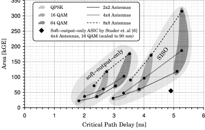
Figure 4: Parametrization design space of the proposed STS SD architecture. Area is measured in gate equivalents (GEs). One GE corresponds to the area of a two-input drive-one NAND gate.

By enabling soft-input processing for the $4\times 4$ 16-QAM reference, the area increases by 57 % from 61 kGates to 96 kGates, while the clock frequency degrades by 34 % from 379 MHz to 250 MHz. We can conclude that the additional cost for soft-input is affordable at the prospect of working at lower SNR regimes with iterative systems.

The proposed architecture scales almost linearly with $M_{\textrm{T}}$ in terms of area. The critical path degrades only by less than 10 % when doubling $M_{\textrm{T}}$. When increasing the QAM order by a factor of 4 in the soft-input case, the area is less than doubled while the frequency degrades by less than 20-25 %, despite the enumeration being significantly affected.

VI Conclusion

To our best knowledge, we introduced the first SISO STS SD architecture, enabling iterative STS SD-based receivers. The parametrized architecture offers very good scalability over $M_{\textrm{T}}$ and the QAM order. The approximate hybrid-enumeration method enables the implementation of iterative STS-based MIMO receivers, although high data-rate communication systems may require multiple parallel SD instances to meet the throughput constraints. We believe that the algorithms and hardware-design principles presented in this paper are suitable for most kinds of SD architectures. Our future development will focus on further enhancements of the architecture, based for instance on the ideas proposed in [6].

VII Acknowledgement

The authors would like to thank Chun-Hao Liao, I-Wei Lai, Martin Senst, David Kammler, Andreas Minwegen, Uwe Deidersen, Konstantinos Nikitopoulos, Dan Zhang, Jeronimo Castrillon, Torsten Kempf, all reviewers and the editor for their valuable feedback and support.

References

• [1] B. Hochwald and S. ten Brink, “Achieving near-capacity on a multiple-antenna channel,” IEEE Trans. Commun., vol. 51, no. 3, pp. 389–399, March 2003.
• [2] S. Chen and T. Zhang, “Low power soft-output signal detector design for wireless MIMO communication systems,” in ISLPED ’07: Proc. of the 2007 international symposium on low power electronics and design.   New York, NY, USA: ACM, August 2007, pp. 232–237.
• [3] M. Li et al., “Selective spanning with fast enumeration: A near maximum-likelihood MIMO detector designed for parallel programmable baseband architectures,” in Proc. IEEE International Conference on Communications ICC ’08, May 2008, pp. 737–741.
• [4] S. Laraway and B. Farhang-Boroujeny, “Implementation of a markov chain monte carlo based multiuser/mimo detector,” IEEE Trans. Circuits Syst. I, vol. 56, no. 1, pp. 246–255, January 2009.
• [5] C. Studer and H. Bölcskei, “Soft-input soft-output single tree-search sphere decoding,” June 2009. http://arxiv.org/abs/0906.0840
• [6] C. Studer, A. Burg, and H. Bölcskei, “Soft-output sphere decoding: algorithms and VLSI implementation,” IEEE J. Sel. Areas Commun., vol. 26, no. 2, pp. 290–300, February 2008.
• [7] B. Mennenga and G. Fettweis, “Search sequence determination for tree search based detection algorithms,” in Proc. IEEE Sarnoff Symposium, April 2009, pp. 1–6.
• [8] C.-H. Liao et al., “Combining orthogonalized partial metrics: Efficient enumeration for soft-input sphere decoder,” in Proc. IEEE 20th International Symposium on Personal, Indoor and Mobile Radio Communications, September 2009.
• [9] C. P. Schnorr and M. Euchner, “Lattice basis reduction: improved practical algorithms and solving subset sum problems,” Math. Program., vol. 66, no. 2, pp. 181–199, August 1994.
• [10] D. Wübben et al., “Efficient algorithm for decoding layered space-time codes,” Electronics Letters, vol. 37, no. 22, pp. 1348–1350, October 2001.
• [11] C. Hess et al., “Reduced-complexity MIMO detector with close-to ML error rate performance,” in Proc. of the 17th ACM Great Lakes Symposium on VLSI (GLSVLSI), March 2007, pp. 200–203.