Optical absorption spectra of finite systems from a conserving Bethe-Salpeter equation approach

Abstract

We present a method for computing optical absorption spectra by means of a Bethe-Salpeter equation approach, which is based on a conserving linear response calculation for electron-hole coherences in the presence of an external electromagnetic field. This procedure allows, in principle, for the determination of the electron-hole correlation function self-consistently with the corresponding single-particle Green function. We analyze the general approach for a “one-shot” calculation of the photoabsorption cross section of finite systems, and discuss the importance of scattering and dephasing contributions in this approach. We apply the method to the closed-shell clusters Na₄, Na${}^{+}_{9}$ and Na${}^{+}_{21}$, treating one active electron per Na atom.

I Introduction

Optical absorption spectra are a widely used and versatile tool for the characterization of the electronic properties of systems of interacting electrons, including their elementary excitations in condensed-matter systems as well as in molecules and clusters. The information that can be obtained from absorption and transmission spectra complements the information accessible from photoelectron spectroscopy techniques, but the interpretation is more difficult because transitions in the interacting system are probed, and the correlated dynamics of electrons and holes in the many-electron system has to be taken into account in order to compare with experiments and to identify spectral characteristics.

In a quasiparticle picture, the photoabsorption is determined by the probability of an electronic transition from an occupied to an empty (or virtual) quasiparticle state, and can be directly determined from the electron-hole correlation function. The determination of the ele-tron-hole correlation function is numerically demanding and usually effected by time-dependent density functional theory (TD-DFT) or by solving the Bethe-Salpeter (BS) integral equation derived in the framework of many-body perturbation theory OnidaRevModPhys .

In the latter approach, the BS equation is often used at the level of a random-phase approximation (RPA), and a popular choice for the calculation of the the excited states, which are needed as input for the BS equation, is the GW approximation for the self-energy, i.e., the effective interaction seen by one particle in the presence of the other carriers. (Here, $G$ is the single-particle Green function and $W$ the screened interaction.)

In the case of state-of-the-art BS equation approaches OnidaPRL ; ShirleyPRL ; RohlfingLouie1 , which may be applied to extended and finite systems, the DFT single-particle states are used as input to GW calculations to obtain the quasiparticle correction to the Kohn-Sham eigenvalues. Then the equation for the electron-hole correlation is transformed into an eigenvalue problem, from which the real parts of the electron-hole transition energies are obtained. The numerical calculations needed for these Bethe-Salpeter approaches are simplified if one assumes an instantaneous, i.e., statically screened, electron-hole interaction for the direct part of the integral kernel of the BS equation. This approach works well with quite a few extended systemes, such as semiconductors and insulators. The straightforward inclusion of the full dynamic screening in the BS equation complicates its numerical solution tremendously, but it is possible to perform an expansion of the dynamically screened potential in plasmonic modes RohlfingPRB . Dynamic screening is also responsible for excitonic effects even in metals, such as Cu and Ag MariniDelSolePRL . General attacks on the problem of dynamic screening in the BS equation go back to the Shindo approximation Shindo . More recently this problem has been reexamined in the framework of nonequilibrium Green function theory, which allows one to derive a Dyson equation for the two-particle propagator BornathKrempSchlanges .

In addition to standard BS equations there also exist explicitly time-dependent (nonequilibrium) Green function based methods, which reduce to the BS equation at the GW-RPA level as a special case, but have been solved for simpler systems using more complicated two-particle correlations than those contained in the GW-RPA theDutchGuy ; AlmbladhPRL . It has also been demonstrated that Green function approaches going beyond the GW-RPA accurately determine the electronic energy renormalizations and broadening for collective excitations in extended systems Kwong-Bonitz ; KochRMP .

In finite systems, electronic states and electron-hole transitions contributing to the absorption spectra are discrete, and are explicitly treated as such in most Green function based theories as well as configuration-interaction (CI) and TD-DFT calculations. However, the experimental signatures due to the discrete states and transition energies invariably appear with a finite linewidth in photoemission and absorption measurements, respectively, due to the finite detector energy-resolution. In particular, the bunching of levels and transitions in certain energy regions, which occurs with increasing system size, cannot be resolved experimentally and may lead to structures that are much broader than the experimental resolution, so that the underlying contributions from individual states or transitions cannot be distinguished. This is often accounted for by adding a phenomenological broadening, which is usually taken to be the same for all transitions.

The approach of the present paper to the ab-initio calculation of absorption spectra in finite systems uses from the outset a finite broadening for single-particle states, i.e., finite lifetimes, as it is rigorously only the case in extended systems. In addition to the background broadening, however, there result dynamical interaction-induced features in the absorption spectra, namely linewidths and energy shifts, which are closely connected Binder-Koch . We aim here at the consistent inclusion of both transition-energy renormalizations and finite linewidths due to ele-tron-hole correlations for finite systems. We achieve this by deriving an integral equation from a quantum kinetic description of the dynamic electron-hole coherences driven by an external, coherent optical field, including Hartree-Fock (HF) and scattering contributions. Our approach is equivalent to an equation of the BS type for the complex electron-hole correlation function using the HF single-particle energies together with a frequency-dependent integral kernel, which contains correlation effects beyond the static HF contributions Kwong-Bonitz . The finite linewidths in our absorption spectra exceed the “background” single-particle broadening and thus describe interaction induced effects including the formation of new peaks. The broadening in our approach should be distinguished from the artificial broadening in nonequilibrium dynamics AlmbladhPRL . Since we base our derivation on the dynamics of electron-hole coherences Kwong-Bonitz in the interacting system, one can include self-energy effects and thus make the calculation self-consistent. An important property of the present approach is that it is straightforward to incorporate the requirement that the (two-particle) electron-hole correlation function be consistent with the electronic single-particle properties, so that a conserving approximation (in the sense of Baym and Kadanoff) results. This approach fulfils important sum rules by construction BaymKadanoff . For instance, the f-sum rule for the density-density correlation, which can be read as the Thomas-Reiche-Kuhn sum rule for the absorption cross section in finite systems, is directly checked in our numerical calculations. Last, but not least, we point out that including correlation effects in a consistent way by examining the equations for electron-hole coherences makes the interdependence between one- and two-particle properties clear. This approach therefore avoids possible inconsistencies of a two-step procedure of calculating first the single-particle properties, and then solving a BS equation with an effective two-particle interaction, as it is done in state-of-the-art BS equation approaches.

Our approach to the ab-initio calculation of absorption spectra in finite systems is based on a recent development of a “consistent” GW theory for finite systems pal-epjb , and it has been applied to extract structural information from cluster absorption spectra pal-jcp . In the present paper, we are mainly concerned with a detailed discussion of the general method for computing absorption spectra. We restrict ourselves to the derivation of a “one-shot” calculational method using Hartree-Fock energies and a constant “background” broadening. This is appealing for its simplicity, and also because it preserves the distinction between HF and correlation contributions throughout the calculations. The present paper expands on the short discussion given in Ref. pal-jcp , and a few illustrative applications to small metal clusters, such as Na₄, Na${}^{+}_{9}$ and Na${}^{+}_{21}$, which exhibit rather complicated correlation mechanisms between the interacting electrons and which develop true collective excitations with increasing clusters size.

II Theory

In this Section we provide the derivation of the equation for the electron-hole correlation function, which determines the photoabsorption cross section. We start by summarizing the connection between these quantities. We then provide the definitions and important properties of the electron-hole correlation functions in Sec. II.1 using non-equilibrium Green function theory. Sec. II.2 contains the derivation of the dynamical equation for the electron-hole coherence in the nonequilibrium formalism, and in Sec. II.3 this result is translated back into a two-particle equation for the electron-hole correlation function.

The central quantity for the calculation of the optical absorption is the retarded density-density correlation function

$$\chi^{\mathrm{r}}(\vec{r},t;\vec{r}^{\prime},t^{\prime})=\langle\rho(\vec{r},t)\rho(\vec{r}^{\prime},t^{\prime})\rangle-\langle\rho(\vec{r},t)\rangle\langle\rho(\vec{r}^{\prime},t^{\prime})\rangle$$ (1)

where $\rho(\vec{r},t)=\psi^{{\dagger}}(\vec{r},t)\psi(\vec{r},t)$ is the particle density operator, expressed by creation and annihilation operators $\psi^{{\dagger}}$ and $\psi^{{\dagger}}$, respectively. We use the expansion

$$\chi^{\mathrm{r}}(\vec{r},t;\vec{r^{\prime}},t^{\prime})=\sum_{n_{1}\dots n_{4}} \langle n_{1}n_{3}|\chi^{\mathrm{r}}(t,t^{\prime})|n_{2}n_{4}\rangle$$ (2)

$$\times \varphi^{*}_{n_{1}}(\vec{r})\varphi_{n_{2}}(\vec{r})\varphi^{*}_{n_{3}}(\vec{r}^{\prime})\varphi_{n_{4}}(\vec{r}^{\prime})$$

in a basis of molecular orbitals $\{\varphi_{n}(\vec{r})\}$, where $n$ labels the orbital. The density-density correlation also describes the linear response of the system to weak perturbation, which is described here by the coupling of a field, with matrix element in the orbital basis $U_{n_{1}n_{2}}(t)$, to the system Hamiltonian $H_{\mathrm{sys}}$ via $H(t)=H_{\mathrm{sys}}+H_{\mathrm{ext}}(t)$ with

$$H_{\mathrm{ext}}(t)=\sum_{n_{1},n_{2}}\rho_{n_{1}n_{2}}(t)U_{n_{1}n_{2}}(t).$$ (3)

The matrix element occurring in Eq. (2) can be expressed as the functional derivative

$$\langle n_{2}n_{1}|\chi^{\mathrm{r}}(t,t^{\prime})|n_{3}n_{4}\rangle=\left.\frac{\delta\langle\rho_{n_{1}n_{2}}(t)\rangle}{\delta U_{n_{3}n_{4}}(t^{\prime})}\right|_{U=0},$$ (4)

where $\rho_{n_{1}n_{2}}(t)=c_{n_{1}}^{{\dagger}}(t)c_{n_{2}}(t)$ and $c_{n}$ ($c_{n}^{{\dagger}}$) denotes the annihilation (creation) operator for an electron in the orbital $\varphi_{n}$. Since the external field couples only electron and hole states, and in linear response the electronic distribution functions $\rho_{nn}$ are unchanged, the only nonzero elements in Eq. (4) are those with indices that pair occupied (electron) and unoccupied (hole) states, i.e., Eq. (4) is the electron-hole correlation function. The photoabsorption cross section thus takes the form GrabowskiGarciaBennemann

$$\sigma(\omega)=\frac{1}{3}\frac{\omega}{\varepsilon_{0}c}\sum_{n_{1}\dots n_{4}}\mathrm{Im}\langle n_{2}n_{1}|\chi^{\mathrm{r}}(\omega)|n_{3}n_{4}\rangle(\vec{d}_{n_{1}n_{2}}\cdot\vec{d}_{n_{3}n_{4}}),$$ (5)

where

$$\vec{d}_{n_{1}n_{2}}=\int\varphi_{n_{1}}^{\ast}(\vec{r})\,e\vec{r}\,\varphi_{n_{2}}(\vec{r})d^{3}r$$ (6)

are the electric dipole matrix elements in the molecular orbital representation.

II.1 Density-density correlation function

The problem in the determination of the absorption cross section is the calculation of $\chi^{\mathrm{r}}(\omega)$, i.e., the Fourier transformation in $t-t^{\prime}$ of Eq. (4). To obtain directly an equation for $\chi^{\mathrm{r}}(\omega)$, we take the detour of deriving dynamical equations for the density response, which are capable of describing more general non-equilibrium situations, and adapt these for the response to weak perturbations. This approach is already implicit in the original treatment of conserving approximations for the two-particle correlation function BaymKadanoff , and has recently been exploited numerically Kwong-Bonitz ; pal-epjb . The functional derivative in the definition of the response function in Eq. (4) can, in principle, be carried out by solving a dynamical equation for the density $\langle\rho_{nn^{\prime}}(t)\rangle$ in the presence of an external field $U_{nn^{\prime}}(t^{\prime})$. The non-equilibrium dynamics can be calculated in any many-particle formalism; here we use nonequilibrium Green functions Kwong-Bonitz ; BaymKadanoff , because they offer the choice to introduce renormalized quasiparticle properties at the single-particle level. For arbitrary nonequilibrium situations, this formalism yields coupled dynamical equations for kinetic and spectral Green functions, i.e., $G^{<}(t_{1},t_{2})$ and $G^{\mathrm{r}}(t_{1},t_{2})$, which depend on two times, even though we need only the time-diagonal

$$\langle\rho(t)\rangle=-i\hbar G^{<}(t,t)$$ (7)

for the determination of $\chi^{\mathrm{r}}$. Calculating the kinetic and spectral Green functions including their dependence on two times is numerically extremely demanding, so that it is only feasible for simple systems theDutchGuy ; AlmbladhPRL . Instead of such a two-time calculation we would like to determine the optical response of a system at $T=0$ K or in equilibrium in terms of a quasiparticle spectrum, i.e., we would like introduce an approximation that replaces the two-time Green functions by

$$G^{<}(t_{1},t_{2})\to\mbox{} G^{<}(t)\equiv G^{<}(t,t)$$ (8)

$$G^{\mathrm{r}}(t_{1},t_{2})\to\mbox{} G^{\mathrm{r}}(t_{1}-t_{2})$$ (9)

$$=\frac{1}{2\pi}\int G^{\mathrm{r}}(\omega)e^{-i\omega(t_{1}-t_{2})}d\omega$$

In other words, in such an approximation the time dependence $t_{1}-t_{2}$ essential for the quasiparticle spectrum, is separated from the time dependence $t=(t_{1}+t_{2})/2$ essential for the kinetics of the quasiparticles. This is achieved by the generalized Kadanoff-Baym ansatz, which reads

$$G^{\gtrless}_{n_{1}n_{2}}(t_{1},t_{2})=\mbox{} i\hbar\,G_{n_{1}n_{1}}^{\mathrm{r}}(t_{1}-t_{2})\,G^{\gtrless}_{n_{1}n_{2}}(t_{2})$$ (10)

$$\quad-i\hbar\,G^{\gtrless}_{n_{1}n_{2}}(t_{1})\,G_{n_{2}n_{2}}^{\mathrm{a}}(t_{1}-t_{2})\ .$$

We then end up with a kinetic equation for $G^{<}(t)$ that includes the quasiparticle properties via its dependence on $G^{\mathrm{r}}(\omega)$, i.e., the Fourier transform of $G^{\mathrm{r}}$ with respect to $t_{1}-t_{2}$.

In our recent paper, Ref. pal-epjb , we were interested in the determination of the electronic quasiparticle properties, i.e., renormalized electronic energies and electronic lifetimes, in the GW approximation, and used different approximations for the density-density correlation function $\chi$. Here, we summarize the connection of the quasiparticle properties with $\chi$ and the screened Coulomb potential. The quasiparticle properties are directly determined by the interacting Green function

$$\left[G_{0}^{-1}(1,\bar{2})-\Sigma(1,\bar{2})\right]G(\bar{2},1^{\prime})=\delta(1-1^{\prime}),$$ (11)

where a space-time integration, or equivalently, a summation over the single-particle indices and a time integration, for quantities with an overbar is understood. Eq. (11) depends on the non-interacting Green function $G_{0}$ (here taken to be the HF Green function) and the self energy (here taken to be the GW self energy)

$$\Sigma(1,2)=i\hbar G(1,2)W(2,1).$$ (12)

(In the orbital representation, Eq. (12) is given by Eq. (19) below.) In terms of the density-density correlation function, which is equal to the reducible polarization function, the screened interation $W$ is an auxiliary quantity given by

$$W(1,1^{\prime})=v(1,1^{\prime})+v(1,\bar{2})\chi(\bar{2},\bar{3})v(\bar{3},1^{\prime}).$$ (13)

Note that the quasiparticle properties depend on the two-particle correlation function $\chi$ via Eqs. (11)–(13), while the two-particle correlation function depends on the single-particle properties via the generalized Kadanoff-Baym ansatz, so that the single- and two-particle functions are connected and the full problem becomes in principle self-consistent.

The following remark on the role of the orbital representation used above is in order. First of all, since the dipole matrix elements in the HF representation connect electron states, i.e., unoccupied states above the LUMO, with hole states, i.e. occupied states below the HOMO, the quantities $\langle\rho_{n_{1}n_{2}}(t)\rangle$ in Eq. (4) describe coherent electron-hole amplitudes in the presence of an external potential $U$. We will refer to these expectation values, which are nonzero only in non-equilibrium, as electron-hole “coherences.” The definition of these coherences depend on the orbital representation. Here, we always use the representation in HF molecular orbitals. This will prove particularly important in the next section, because it allows us to conveniently separate the HF contribution in the equation for the electron-hole coherence.

II.2 Kinetic equation for the density response

Our general approach to the calculation of the Green function $G$ is discussed in some detail in Ref. pal-epjb . Thus we concentrate here on the derivation of the density-density correlation function. To calculate the action of the weak external field $U$, we start from the equation of motion for $G^{<}(t_{1},t_{2})$ evaluated at equal times $t_{1}=t_{2}=t$ which reads

$$i\hbar \frac{\partial}{\partial t}G^{<}_{n_{1}n_{2}}(t)=$$ (14)

$$\sum_{n_{3}}\Bigl{\{}\left[\,T_{n_{1}n_{1}}\delta_{n_{1}n_{3}}+U_{n_{1}n_{3}}(t)+\Sigma^{\mathrm{HF}}_{n_{1}n_{3}}(t)\,\right]G^{<}_{n_{3}n_{2}}(t,t)$$

$$\quad-G^{<}_{n_{1}n_{3}}(t,t)\left[\,T_{n_{2}n_{2}}\delta_{n_{2}n_{3}}+U_{n_{3}n_{2}}(t)+\Sigma^{\mathrm{HF}}_{n_{3}n_{2}}(t)\right]\Bigr{\}}$$

$$\quad+S_{n_{1}n_{2}}(t).$$

Here, $T$ is the non-interacting part of the Hamiltonian $H_{\mathrm{sys}}=T+V$, and includes the core potential in our case. The scattering contribution describing correlations beyond the mean-field (HF) approximation is given by

$$S_{n_{1}n_{2}}(t)= \sum_{n_{3}}\int_{-\infty}^{t}d\bar{t}\left[\,\Sigma^{>}_{n_{1}n_{3}}(t,\bar{t})\,G^{<}_{n_{3}n_{2}}(\bar{t},t)\right.$$ (15)

$$\left.+G^{<}_{n_{1}n_{3}}(t,\bar{t})\,\Sigma^{>}_{n_{3}n_{2}}(\bar{t},t)-(\gtrless\leftrightarrow\lessgtr)\,\right].$$

Also, the instantaneous HF self-energy

$$\Sigma^{\mathrm{HF}}_{n_{1}n_{2}}(t_{1})= -i\hbar\sum_{n_{3}n_{4}}\langle n_{1}n_{3}|v|n_{2}n_{4}\rangle\,G^{<}_{n_{3}n_{4}}(t_{1},t_{1})$$ (16)

$$+i\hbar\sum_{n_{3}n_{4}}\langle n_{1}n_{2}|v|n_{3}n_{4}\rangle\,G^{<}_{n_{3}n_{4}}(t_{1},t_{1})$$

has been separated from the dynamic correlation contribution via the identity

$$\Sigma^{\mathrm{r}/a}_{n_{1}n_{2}} (t_{1},t_{2})=\Sigma^{\mathrm{HF}}_{n_{1}n_{2}}(t_{1})\,\delta(t_{1}-t_{2})$$ (17)

$$\pm\Theta\left(\pm(t_{1}-t_{2})\right)\big{[}\Sigma^{>}_{n_{1}n_{2}}(t_{1},t_{2})-\Sigma^{<}_{n_{1}n_{2}}(t_{1},t_{2})\big{]}.$$

In Eq. (16) and below, $v$ is the bare Coulomb matrix element, with the index structure defined as

$$\langle n_{1}n_{2}|v|n_{3}n_{4}\rangle=\int d^{3}r_{1}d^{3}r_{2}\,\varphi^{*}_{n_{1}}({\vec{r}}_{1})\varphi^{*}_{n_{2}}({\vec{r}}_{2})$$ (18)

$$\times v(|\vec{r}_{1}-\vec{r}_{2}|)\,\varphi_{n_{3}}({\vec{r}}_{1})\varphi_{n_{4}}({\vec{r}}_{2}).$$

Eq. (17) is quite general and holds regardless of the level of approximation for the self-energy, which determines the functional form of $\Sigma^{\gtrless}$. Due to the separation between the HF and the dynamic correlation contributions to the self-energy, and since we are not attempting a self-consistent calculation, it is natural to use for the basis set functions $\{\varphi_{n}(\vec{r})\}$ the HF molecular orbitals, as opposed to DFT-based approaches that lump the exchange (Fock) and correlation part together, and separate out only the direct (Hartree) contribution to the self-energy.

Specifically, we use the GW approximation for the dynamic correlation contribution

$$\Sigma_{n_{1}n_{2}}^{\gtrless}(t,\bar{t})=i\hbar\sum_{n_{3}n_{4}}G^{\gtrless}_{n_{3}n_{4}}(t,\bar{t})\,\langle n_{1}n_{2}|W^{\lessgtr}(\bar{t},t)|n_{3}n_{4}\rangle$$ (19)

where matrix elements of the screened Coulomb interaction $W$ have been introduced in analogy with Eq. (18). Note that Eq. (19) is just Eq. (12) written in the basis of the HF orbitals.

For the two-time Green functions from the correlation term we employ the generalized Kadanoff-Baym quasiparticle ansatz (10). Note that we have not specified yet which $G^{\mathrm{r}}(t-\bar{t})$ we use to describe the spectral properties of the electrons. If one uses the results of a GW calculation, the calculation becomes self consistent, because the screened interaction depends on $\chi$. We do not intend to pursue the self-consistent problem further in the present paper, so that we neglect the correlation corrections to the HF single-particle properties in the following. With this approximation the retarded and advanced Green functions at the HF level are given by

$$i\hbar\,G_{n_{1}n_{1}}^{\mathrm{r\ (HF)}}(t-\bar{t})=\Theta(t-\bar{t})\exp\{-\frac{i}{\hbar}\tilde{\epsilon}_{n_{1}}(t-\bar{t})\}.$$ (20)

For clusters, the corrections to the ground-state energies are expected to be small so that a Green function constructed from HF eigenvalues constitutes a reasonable starting point. A non-zero quasiparticle broadening $\gamma$ ensures the proper behavior of the HF retarded and advanced Green functions, and we use here and in the following the notation $\tilde{\epsilon}_{n}=\epsilon^{\mathrm{HF}}_{n}-i\gamma$. With this approximation, Eq. (14) is a kinetic equation for the density response, which has a parametric dependence of the electronic quasiparticle properties via Eqs. (15)–(20) and which is closed in the sense that it does not depend on Green functions with off-diagonal time arguments.

Before we can actually compute $\chi^{\mathrm{r}}$ as the functional derivative of Eq. (14) we need a few more steps. The functional derivative essentially captures the linear dependence of the density on the external potential $U$. To first order in $U$, or, equivalently, for a weak external potential, only density fluctuations, i.e., $\langle\rho_{nn^{\prime}}(t)\rangle=-i\hbar G^{<}_{nn^{\prime}}(t,t)$ with $n\neq n^{\prime}$, are influenced by the field, whereas the distribution functions $f_{n}(t)=\langle\rho_{nn}(t)\rangle$ are unchanged and therefore time-independent. Specializing to the case of such a weak $U$ we can rewrite Eq. (14) as

$$\big{(}i\hbar\frac{\partial}{\partial t}-\epsilon_{n_{1}}^{\mathrm{HF}}+\epsilon_{n_{2}}^{\mathrm{HF}}\big{)}G_{n_{1}n_{2}}^{<}(t)+(f_{n_{1}}-f_{n_{2}})\Bigl{[}\frac{i}{\hbar}U_{n_{1}n_{2}}(t)$$

$$+\sum_{n_{3}n_{4}}\big{(}\langle n_{1}n_{3}|v|n_{2}n_{4}\rangle-\langle n_{1}n_{2}|v|n_{3}n_{4}\rangle\big{)}G_{n_{3}n_{4}}^{<}(t)\Bigr{]}$$

$$\qquad=S_{n_{1}n_{2}}(t).$$ (21)

Here, we have introduced the HF eigenvalues $\epsilon_{n_{1}}^{\mathrm{HF}}$ and distributions $f_{n}=f(\epsilon_{n}^{\mathrm{HF}})$ where $f(\hbar\omega)$ denotes the Fermi function, so that $f_{n}$ is equal to 1 for occupied and 0 for unoccupied states at $T=0$ K. In Eq. (II.2), $S$ stands for the scattering term of Eq. (15), which includes now the generalized Kadanoff-Baym ansatz. With the assumption of a weak external field, we should also consistently linearize the scattering term with respect to the $G^{\gtrless}_{n\neq n^{\prime}}$ and replace factors of $G^{<}_{nn}(t,t)$ by their equilibrium value, $i\hbar f(\epsilon_{n}^{\mathrm{HF}})$. With these modifications, the linearized kinetic Eq. (II.2) for the density response assumes a form, for which we can compute the functional derivative.

II.3 Bethe-Salpeter equation for $\chi^{\mathrm{r}}$

The equation for $\chi^{\mathrm{r}}(t,t^{\prime})$ is obtained by functional differentiation of Eq. (II.2) with respect to $U(t^{\prime})$ and letting $U\to 0$ afterwards. This is done by replacing everywhere the term $\delta G_{n_{1}n_{2}}^{<}(t)/\delta U_{n_{3}n_{4}}(t^{\prime})$ with $-i\hbar\langle n_{1}n_{2}|\chi^{\mathrm{r}}(t-t^{\prime})|n_{3}n_{4}\rangle$, cf. Eq. (4). Apart from the $\delta G/\delta U$, functional differentiation of Eq. (II.2) also yields contributions of the form $\delta W/\delta U$ but these are neglected, in agreement with other GW based approaches LouiedWdU . The result depends only on $t_{1}-t_{2}$, and we can Fourier transform in the time difference to obtain the frequency-dependent $\chi^{\mathrm{r}}(\omega)$ in the form

$$\big{(}\hbar\omega-\epsilon_{n_{1}}^{\mathrm{HF}}+\epsilon_{n_{2}}^{\mathrm{HF}}\big{)}\langle n_{1}n_{2}|\chi^{\mathrm{r}}(\omega)|n_{3}n_{4}\rangle$$ (22)

$$\qquad+\,(f_{n_{1}}-f_{n_{2}})\Big{[}\delta_{n_{1}n_{3}}\delta_{n_{2}n_{4}}+$$

$$\sum_{n_{5}n_{6}}\Big{(}\langle n_{1}n_{5}|v|n_{2}n_{6}\rangle-\langle n_{1}n_{2}|v|n_{5}n_{6}\rangle\Big{)}\langle n_{5}n_{6}|\chi^{\mathrm{r}}(\omega)|n_{3}n_{4}\rangle\Big{]}$$

$$\qquad+\sum_{n_{5}n_{6}}\langle n_{1}n_{2}|\Delta(\omega)|n_{5}n_{6}\rangle\langle n_{5}n_{6}|\chi^{\mathrm{r}}(\omega)|n_{3}n_{4}\rangle=0$$

with the correlation kernel

$$\langle n_{1}n_{2} |\Delta(\omega)|n_{3}n_{4}\rangle=$$

$$\sum_{n_{5}n_{6}}\Big{[} \frac{f_{n_{1}}(1-f_{n_{5}})f_{n_{6}}+(1-f_{n_{1}})f_{n_{5}}(1-f_{n_{6}})}{\hbar\omega-\epsilon^{\mathrm{HF}}_{n_{6}}+\epsilon^{\mathrm{HF}}_{n_{5}}-\epsilon^{\mathrm{HF}}_{n_{1}}+\epsilon^{\mathrm{HF}}_{n_{4}}+i(\gamma_{n_{1}}+\gamma_{n_{4}})}$$

$$\qquad\times\langle n_{1}n_{5}|v|n_{3}n_{6}\rangle\langle n_{6}n_{2}|v|n_{5}n_{4}\rangle$$

$$+ \frac{f_{n_{2}}(1-f_{n_{5}})f_{n_{6}}+(1-f_{n_{2}})f_{n_{5}}(1-f_{n_{6}})}{\hbar\omega+\epsilon^{\mathrm{HF}}_{n_{6}}-\epsilon^{\mathrm{HF}}_{n_{5}}-\epsilon^{\mathrm{HF}}_{n_{3}}+\epsilon^{\mathrm{HF}}_{n_{2}}+i(\gamma_{n_{3}}+\gamma_{n_{2}})}$$

$$\qquad\times\langle n_{1}n_{5}|v|n_{3}n_{6}\rangle\langle n_{6}n_{2}|v|n_{5}n_{4}\rangle$$

$$-\delta_{n_{1}n_{3}} \sum_{n_{7}}\frac{f_{n_{7}}(1-f_{n_{6}})f_{n_{5}}+(1-f_{n_{7}})f_{n_{6}}(1-f_{n_{5}})}{\hbar\omega-\epsilon^{\mathrm{HF}}_{n_{6}}+\epsilon^{\mathrm{HF}}_{n_{5}}-\epsilon^{\mathrm{HF}}_{n_{3}}+\epsilon^{\mathrm{HF}}_{n_{7}}+i(\gamma_{n_{3}}+\gamma_{n_{7}})}$$

$$\qquad\times\langle n_{4}n_{5}|v|n_{7}n_{6}\rangle\langle n_{6}n_{2}|v|n_{5}n_{7}\rangle$$

$$-\delta_{n_{2}n_{4}} \sum_{n_{7}}\frac{f_{n_{7}}(1-f_{n_{6}})f_{n_{5}}+(1-f_{n_{7}})f_{n_{6}}(1-f_{n_{5}})}{\hbar\omega+\epsilon^{\mathrm{HF}}_{n_{6}}-\epsilon^{\mathrm{HF}}_{n_{5}}-\epsilon^{\mathrm{HF}}_{n_{7}}+\epsilon^{\mathrm{HF}}_{n_{4}}+i(\gamma_{n_{7}}+\gamma_{n_{4}})}$$

$$\qquad\times\langle n_{1}n_{5}|v|n_{7}n_{6}\rangle\langle n_{6}n_{3}|v|n_{5}n_{7}\rangle\Big{]}.$$ (23)

The functional form of Eq. (22) for $\chi^{\mathrm{r}}$ allows one to draw conclusions how many-particle effects will show up in the calculated absorption spectra. Note first that the direct and exchange Coulomb contributions renormalize the transition energies together with the real part of the correlation (or scattering) contribution $\Delta$. The imaginary part of $\Delta$ describes an interaction-induced dephasing of electron-hole coherences driven by $U$. Thus the imaginary part of $\Delta$ determines the line broadening of the absorption resonances. Note that the complex quantity $\Delta$ contains contributions to resonance shifts as well as the broadening; both effects are therefore related. The renormalization/broadening contributions $\Delta$ are determined by a coupling of each electron-hole transition to all other transitions due to the Coulomb interaction. Although the single-particle broadening $\gamma$ (inverse lifetime) of each electron or hole state, or more generally, the single-particle spectral functions, influence the broadening of the transitions, Eq. (II.3) shows that this influence is not described by a simple convolution of the electron and hole lifetimes. Rather, the line broadening for all absorption resonances arises due to an interaction-induced coupling of individual electron-hole transitions. The “collective” origin of the damping should be distinguished from the question whether a given resonance is due to collective electron-hole excitations, such as excitons or plasmons, or whether it mainly stems from a single electron-hole transition.

III Results

In this Section, we apply Eqs. (5) and (22) together with Eq. (II.3) to compute the photoabsorption cross sections for the clusters Na₄, Na${}_{9}^{+}$ and Na${}_{21}^{+}$ and we compare our calculations with experimental results. The photoabsorption cross section of Na₄, Na${}_{9}^{+}$ and Na${}_{21}^{+}$ has been calculated by different approaches, including: the jellium model approach Ekardt2 ; Ekardt3 ; KummelBrackReinhardPRB ; BrackRMP ; RomanPRB ; PachecoPRL , highly correlated quantum chemistry methods such as multireference (double) CI BonacicChemRev , a combination of GW and BS equation approaches OnidaNa4 , time-dependent density-functional theory (TD-DFT) in the local density approximation (LDA) Ogut and beyond LDA with sophisticated exchange-correlation functionals MarquesCastroRubio . Another approach, which has been applied to calculate the photoabsorption cross section of small sodium cations (including Na${}_{9}^{+}$), is the TD-LDA (including generalized gradient corrections) used along phase-space trajectories obtained within finite-temperature Born-Oppenheimer local spin density molecular dynamics UziPRL .

We focus on the influence of correlation effects due to the Coulomb interaction between the electrons from the outermost electronic shell of the Na ions at $T=$0 K, and employ the frozen-phonon approximation, so that the geometrical structure of the clusters is fixed at the energetically optimized configuration. Both core-shell electrons and electrons from the outermost shell influence the many-particle states of the interacting electron system and thus the optical spectra. However, because the core electron states are energetically well separated from the outermost shell, these states are only weakly mixed into the electronic states contributing to transitions in the energy window of interest, which is a few eVs, and we expect that the core electrons only introduce an additional fine structure in the optical spectrum in that window. For the clusters investigated here, we therefore treat one active electon per Na atom and use effective core potentials to describe the contribution of the core electrons. If one is interested in accounting for processes involving electrons from inner shells a two-particle-hole Tamm-Dancoff approximation Schirmer2 or an algebraic diagrammatic construction Schirmer4 may be used to describe ionization and double ionization processes in the inner valence region.

We treat here only closed-shell systems although, in principle, the theory is applicable to any finite system as the index $n$ refers to a molecular orbital that can be from an open shell system as well. Since we are interested in the absorption lineshapes and interaction induced shifts due to electronic correlation effects, we view the structure optimization of the cluster geomtry, and the necessary quantum-chemistry only as a tool. A relatively simple approach that fits well with our method is to obtain the HF eigenfunctions and the optimization of the underlying cluster geometries from a restricted HF calculation YaroslavHubner performed with the GAUSSIAN 03 quantum chemistry package gaussian03 . In our calculations, the $3s^{1}$ valence electron of each Na atom is explicitly treated using the lanl2dz basis set: a double zeta basis set of Gaussian-like atomic orbitals in the (3s3p/2s2p) contraction and relativistic Los Alamos LosAlamos effective core potential (ECP) for the core electrons. The structure optimization of the clusters starts from geometry configurations taken from Refs. KummelBrackReinhardPRB ; BonacicChemRev ; UziPRL ; IshiiPRB .

For the computation of the correlation contribution $\Delta$ from Eq. (II.3) we use $\gamma$=0.25 eV for the quasiparticle energies $\tilde{\epsilon}=\epsilon-i\gamma$. The value for $\gamma$ used here is slightly modified from our earlier GW results, where we obtained for energetically low occupied states 0.085 eV for Na${}_{9}^{+}$ and 0.29 eV for Na${}_{21}^{+}$ pal-epjb . However, this choice simplifies the numerical calculation because it makes it easier to carry out the sums over complicated energy denominators, and makes $\Delta(\omega)$ a smoother function of $\omega$. We stress that introducing a fixed quasiparticle broadening for the calculation of $\Delta(\omega)$ does not mean that we are fixing the broadening of the resonances in $\chi^{\mathrm{r}}$ to this value. Rather, the resonance broadening, which is responsible for the finite width of the peaks in the absorption spectrum, is due to the imaginary part and the complicated index dependence of the full correlation kernel $\Delta(\omega)$.

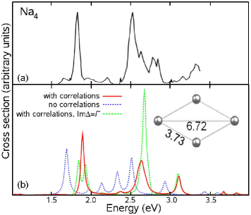
Figure 1: Measured (a) and computed (b) absorption cross section for Na₄. The experimental result is adapted from Ref. Na4EXP . The theoretical results are obtained with (solid line) and without (dotted line) correlation contributions in the equation for $\chi^{\rm r}$. The spectrum obtained using only the real part (plus a constant imaginary part) of the correlation term is also shown (dashed line). The inset shows the cluster geometry with distances in Å.

Figure 1 shows the computed absorption cross section for Na₄ together with the experimental result from Ref. Na4EXP . The main measured peaks which occur around 1.8 and 2.5 eV are well resolved by the theoretical spectrum when $\chi^{\rm r}$ is calculated by Eqs. (22) and (II.3). To emphasize the importance of the correlation contribution, we compare this with the cross section calculated using a constant, phenomenological broadening for each transition. Technically, this is achieved by using Eq. (22) with a constant, diagonal broadening, i.e.,

$$\langle n_{1}n_{2}|\Delta(\omega)|n_{5}n_{6}\rangle=i\delta_{n_{1}n_{5}}\delta_{n_{2}n_{6}}\Gamma.$$ (24)

where we have assumed $\Gamma=0.03$ eV. Using the phenomenological broadening, the absorption cross section does not compare well with the experimental data as regards the position and the shape of the lines. Only the inclusion of the full correlation term yields good agreement between the calculated and the measured spectra. This result illustrates that the shift of the absorption resonances due to the real part of correlation contributions can be on the order of several tenths of eVs and this shift is needed to obtain agreement with experiment. In addition to the shift, the imaginary part of $\Delta$, which is responsible for the broadening, redistributes spectral weight between the different peaks and leads to an overall very different shape of the absorption spectrum for the two cases. To disentangle the effect of the broadening on the redistribution of the spectral weight, we have performed a calculation with only the real part of $\Delta$, plus a diagonal broadening. This yields a splitting of the peak at 1.8 eV into two new peaks. Also, the peak at 2.5 eV is blue-shifted and now contains most of the spectral weight. This is in agreement with results for extended system, where it is known that the broadening and level shifts in this type of complex BS equation are closely connected and cannot be separated by taking into account the real or imaginary part only.

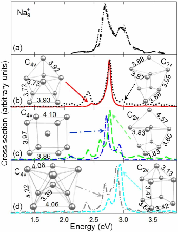
Figure 2: Measured (a) and calculated absorption cross sections for Na${}_{9}^{+}$. The experimental results are adapted from Ref. Na921EXP . The spectra (b)–(d) are calculated for six different cluster geometries. The insets show the cluster geometries with distances in Å.

When comparing experimental and theoretical results one should keep in mind that the geometry configuration, which we obtain by structural optimization, is important for the calculation, but not well known for the clusters studied in the experiment. Moreover, finite temperature and inhomogeneous broadening effects in experiments wash out the intrinsic spectral features. To account for the finite temperature effects and for the unknown cluster geometries which might occur in experiment, we have considered six different configurations for Na${}_{9}^{+}$ with low ground state energy: three structures with C_4v symmetry and three with C_2v symmetry, see Fig. 2. The total ground state energies of the clusters differ by less than 0.3 eV. The comparison between the measured (from Ref. Na921EXP ) and the calculated spectra is shown in Fig. 2. The experimental spectra exhibit a splitting of the main absorption line into a larger peak centered around 2.68 eV and a smaller peak around 2.98 eV. For all the clusters considered here, the main absorption lines occur in the same energy interval as the measured lines, but the shape of the peaks does not compare as well with experiment as in the case of Na₄. Both the C_4v and the C_2v clusters from panel (b) of Fig. 2 yield a single large peak at 2.74 eV. The C_4v cluster from panel (c) reproduces best the experiment with respect to the position and the shape of the absorption lines. Also, the C_2v cluster from panel (d) of Fig. 2 is capable of resolving the smaller experimental peak at 2.98 eV, but the larger experimental peak at 2.68 eV is not present in the theoretical spectrum. In an experiment, clusters with different configurations may contribute to the shape of the absorption spectrum, but the weight of the contributions due to different possible configurations cannot be determined from experiment nor from a $T=0$ K theory. Given the potential problems for experiment-theory comparisons, we find a good overall agreement between the measured and the calculated spectra of Na${}_{9}^{+}$.

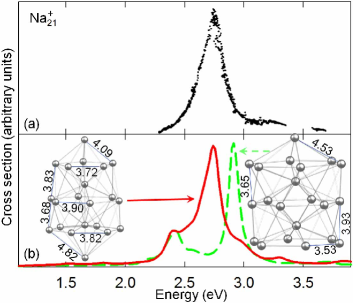
Figure 3: Measured (a) and computed (b) absorption cross section for Na${}_{21}^{+}$. The experimental result is adapted from Ref. Na921EXP . The theoretical spectra are calculated for the prolate cluster (solid line), and the structure with C_6v symmetry (dashed line). The insets show the cluster geometries with distances in Å.

Figure 3 shows the comparison between the experimental and the theoretical cross section of Na${}_{21}^{+}$. The measured spectrum displays a large absorption line centered around 2.74 eV Na921EXP . Two different cluster geometries were used in the calculation: one corresponding to a prolate (i.e., elongated) cluster and one structure with C_6v symmetry. The qualitative agreement between theory and experiment is very good with respect to the position and the shape of the peak for the prolate Na${}_{21}^{+}$. For the cluster with C_6v symmetry the agreement is not that good, although the main peaks are situated in the experimental 2.3–3.2 eV energy interval.

The different quality of the agreement between theory and experiment for the Na₄ and Na${}_{21}^{+}$ clusters is also an indication that cluster size plays an important role: For small clusters, the geometrical configuration is relatively well defined, and the photoabsorption cross section is characterized by a few discrete resonances. In the other extreme, when the system contains a large number of atoms there are many more overlapping individual electron-hole transitions, so that the resonances are not well resolved. Moreover, there may be different geometrical configurations with similar total energies, which may contribute to the experimental spectrum. For Na${}_{9}^{+}$, we are neither in the limit of a small nor a larger cluster so that there is a competition between the two trends: the spectral density of the single electron-hole transitions is not yet large enough as to yield featureless broadened peaks, but the number of the possible configurations with different electronic properties is large enough so that so that the cluster geometry present in the experiment is difficult to predict.

Finally we wish to point out that we have checked numerically that all the computed spectra shown fulfill the f-sum rule for finite systems to better than 99%

$$\frac{1}{3}\int d\omega\,\omega \sum_{n_{1}\dots n_{4}}(\vec{d}_{n_{1}n_{2}}\cdot\vec{d}_{n_{3}n_{4}})$$ (25)

$$\times{\rm Im}\langle n_{2}n_{1}|\chi^{\rm r}(\omega)|n_{3}n_{4}\rangle=-\frac{\hbar^{2}\pi}{m}N_{e},$$

where $m$ is the electron mass and $N_{e}$ is the total number of electrons in the system. Eq. (25) is the Thomas-Reiche-Kuhn sum rule for the absorption cross section and is a measure for the overall quality of the absorption spectrum.

IV Conclusions

We have presented an approach to compute the absorption spectra for finite systems based on a linear response theory for the dynamical electron-hole coherences in the presence of an external field. Using a quasiparticle ansatz in the quantum kinetic equation for the electron-hole coherence, which includes HF and scattering contributions, allows us to derive a BS equation for the electron-hole correlation function with a complex, frequency-dependent kernel. The latter is determined by the scattering (or correlation) contributions to the electron-hole coherence dynamics. One thus obtains absorption spectra that include level-shifts of transition energies and a broadening of the absorption peaks due to electronic interactions. The correlation induced shifts and the broadening are closely related since they are the result of the complex, frequency dependent kernel, and the broadening mimics the bunching of discrete levels in finite systems. We apply the method to three important Na clusters: Na₄ and the magic number clusters Na${}_{9}^{+}$ and Na${}_{21}^{+}$, and compare both the calculated resonance energies and the shape of the absorption lines with experimental results.

G.P. and W.H. acknowledge support through the Priority Programme 1153 of the German Research Foundation.

References

- (1) G. Onida, L. Reining, and A. Rubio, Rev. Mod. Phys. 74, (2002) 601.
- (2) S. Albrecht, L. Reining, R. Del Sole, and G. Onida, Phys. Rev. Lett. 80, (1998) 4510.
- (3) L. X. Benedict, E. L. Shirley, and R. B. Bohn, Phys. Rev. Lett. 80, (1998) 4514.
- (4) M. Rohlfing and S. G. Louie, Phys. Rev. Lett. 81, (1998) 2312.
- (5) M. Rohlfing and S. G. Louie, Phys. Rev. B 62, (2000) 4927.
- (6) A. Marini and R. Del Sole, Phys. Rev. Lett. 91, (2003) 176402.
- (7) K. Shindo, J. Phys. Soc. Jpn. 29, (1970) 278.
- (8) Th. Bornath, D. Kremp, and M. Schlanges, Phys. Rev. E 60, (1999) 6382.
- (9) N. E. Dahlen and R. van Leeuwen, Phys. Rev. Lett. 98, (2007) 153004.
- (10) M. Puig von Friesen, C. Verdozzi, and C.-O. Almbladh, Phys. Rev. Lett. 103, (2010) 176404.
- (11) N.-H. Kwong and M. Bonitz, Phys. Rev. Lett. 84, (2000) 1768.
- (12) G. Khitrova, H. M. Gibbs, F. Jahnke, M. Kira, and S. W. Koch, Rev. Mod. Phys. 71, (1999) 1591.
- (13) R. Binder and S. W. Koch, Progr. Quantum Electr. 19, (1995) 307.
- (14) G. Baym and L. P. Kadanoff, Phys. Rev. 124, (1961) 287.
- (15) G. Pal, Y. Pavlyukh, H. C. Schneider, and W. Hübner, Eur. Phys. J. B 70, (2009) 483.
- (16) G. Pal, G. Lefkidis, , H. C. Schneider, and W. Hübner, J. Chem. Phys. 133, (2010) 154209.
- (17) S. Grabowski, M. E. Garcia, and K. H. Bennemann, Phys. Rev. Lett. 72, (1994) 3969.
- (18) S. Ismail-Beigi and S. G. Louie, Phys. Rev. Lett. 90, (2003) 076401.
- (19) W. Ekardt, Phys. Rev. Lett. 52, (1984) 1925.
- (20) W. Ekardt, Phys. Rev. B 31, (1985) 6360.
- (21) S. Kümmel, M. Brack, and P.-G. Reinhard, Phys. Rev. B 62, (2000) 7602.
- (22) M. Brack, Rev. Mod. Phys. 65, (677) 1993.
- (23) F. Alasia, L. Serra, L., R. A. Broglia, N. Van Giai, E. Lipparini, and H. E. Roman, Phys. Rev. B 52, (1995) 8488.
- (24) J. M. Pacheco and W. D. Schöne, Phys. Rev. Lett. 79, (1997) 4986.
- (25) V. Bonačić-Koutecký, P. Fantucci, and J. Koutecký, Chem. Rev. 91, (1991) 1035.
- (26) G. Onida, L. Reining, R. W. Godby, R. Del Sole, and W. Andreoni, Phys. Rev. Lett. 75, (1995) 818.
- (27) I. Vasiliev, S. Öğüt, and J. R. Chelikowsky, Phys. Rev. Lett. 82, (2001) 1919.
- (28) M. A. L. Marques, A. Castro, and A. Rubio, J. Chem. Phys. 115, (2001) 3006.
- (29) M. Moseler, H. Häkkinen, and U. Landman, Phys. Rev. Lett. 87, (2001) 053401.
- (30) L. S. Cederbaum, W. Domcke, J. Schirmer, and W. von Niessen, Adv. Chem. Phys. 65, (1986) 115.
- (31) J. Schirmer, L. S. Cederbaum, and O. Walter Phys. Rev. A 28, (1983) 1237.
- (32) W. D. Knight, K. Clemenger, W. A. de Heer, W.A. Saunders, M.Y. Chou, and M. L. Cohen, Phys. Rev. Lett. 52, (1984) 2141.
- (33) W. A. de Heer, Rev. Mod. Phys. 65, (1993) 611.
- (34) Y.Pavlyukh and Hübner, Phys. Lett. A 327, (2004) 241.
- (35) M. J. Frisch, G. W. Trucks, H. B. Schlegel et al., GAUSSIAN 03 (Gaussian, Inc., Pittsburgh PA, 2003).
- (36) P. J. Hey and W. R. Wadt, J. Chem. Phys. 82, (1985) 284.
- (37) S. Ishii, K. Ohno, Y. Kawazoe, and S. G. Louie, Phys. Rev. B 63, (2001) 155104.
- (38) C. Wang, S. Pollack, D. Cameron, and M. Kappes, Chem. Phys. Lett. 166, (1990) 26.
- (39) T. Reiners, W. Orlik, C. Ellert, M. Schmidt, and H. Haberland, Chem. Phys. Lett. 215, (1993) 357.