Quantifying the connectivity of a network:
The network correlation function method

Abstract

Networks are useful for describing systems of interacting objects, where the nodes represent the objects and the edges represent the interactions between them. The applications include chemical and metabolic systems, food webs as well as social networks. Lately, it was found that many of these networks display some common topological features, such as high clustering, small average path length (small world networks) and a power-law degree distribution (scale free networks). The topological features of a network are commonly related to the network’s functionality. However, the topology alone does not account for the nature of the interactions in the network and their strength. Here we introduce a method for evaluating the correlations between pairs of nodes in the network. These correlations depend both on the topology and on the functionality of the network. A network with high connectivity displays strong correlations between its interacting nodes and thus features small-world functionality. We quantify the correlations between all pairs of nodes in the network, and express them as matrix elements in the correlation matrix. From this information one can plot the correlation function for the network and to extract the correlation length. The connectivity of a network is then defined as the ratio between this correlation length and the average path length of the network. Using this method we distinguish between a topological small world and a functional small world, where the latter is characterized by long range correlations and high connectivity. Clearly, networks which share the same topology, may have different connectivities, based on the nature and strength of their interactions. The method is demonstrated on metabolic networks, but can be readily generalized to other types of networks.

I Introduction

A network, or graph, consists of a set of nodes, from which selected pairs are connected by edges. Such mathematical constructions provide a useful description for systems of interacting objects. More specifically, network concepts are used in the analysis of chemical and metabolic systems as well as food webs and social networks. In recent years, there has been much progress in the analysis of the topology of these networks. The network topology can be characterized by features such as the number of nodes, $J$, and the average degree $\langle[\rangle k]$, namely the average number of edges that are connected to a node. A more detailed description of the network topology is given by the degree distribution, $P(k)$, which is the probability that a randomly selected node has exactly $k$ edges. Another important topological feature measures the tendency of a network to support the formation of cliques. A clique is a fully connected set of nodes, namely each pair of nodes in such a set is connected by an edge. The tendency of a network to form cliques can be characterized by the clustering coefficient Watts1998 ; Wasserman1994 ; Barrat2000 ; Newman2000 . Roughly speaking, when a network has a high clustering coefficient it is considered to be highly connected. A low clustering coefficient implies that the network is only loosely connected.

Networks exhibit a unique metric, in which the distance, $d$, between any two nodes is given by the minimal number of edges one has to cross in order to pass from one node to the other. In some cases, the distance can be used as a measure for the connection between a pair of nodes. This is based on the assumption that two directly reacting nodes ($d=1$) strongly affect each other, whereas distant nodes weakly affect one another. The average path length in a network, $\langle[\rangle d]$, is obtained by averaging over the distance between all pairs of nodes in the network. The parameters defined above were evaluated for random graphs and their dependence on $J$ and $\langle k\rangle$ was found Erdos1959 ; Erdos1960 ; Erdos1961 ; Chung2001 . However, the analysis of realistic networks shows that they are very different from random graphs Barabasi2001 . In realistic networks it is common to find surprisingly low average path lengths, and relatively high clustering coefficients. In many cases the degree distribution follows a power law form, rather than the Poisson distribution which is the signature of random networks. These features were found to appear in social networks Kochen1989 ; Watts1998 ; Newman2001a ; Newman2001b ; Newman2001c ; Barabasi2001 ; Redner1998 ; Vazquez2001 ; Newman2000 ; Barabasi1999 ; Albert2000 ; Amaral2000 , the world wide web Lawrence1998 ; Lawrence1999 ; Albert1999 ; Broder2000 ; Adamic2000 ; Adamic1999 , ecological networks Pimm1991 ; Williams2000 ; Montoya2002 ; Camacho2002a , and metabolic networks Wagner2000 ; Fell2000 ; Jeong2000 .

While the topological properties of realistic networks have been elucidated, the implications on the functionality of these networks are not fully understood. The small average path length and the high clustering of many realistic networks, render them as small world networks. At first glance, the small world characteristics imply that realistic networks function as highly connected systems. Indeed, one expects that if the distance between two nodes is small, the correlation between them will be strong. For instance, in the case of a metabolic network, the concentrations of interacting proteins will strongly depend on each other. A perturbation in the concentration of one protein is likely to affect the concentration of the other. This might lead to the conclusion that small world networks are highly susceptible to local perturbations, as almost all the nodes are just a short distance away. The problem with this topological analysis, is that it does not relate to the specific function of a given network or to the strength of the interactions between its nodes Barabasi2002 . Consider, for instance, a metabolic network and an ecological network sharing the same topology. In what sense can these two networks be regarded as similar networks? Even if the two have the same topological structure, the nature of their functional behavior is fundamentally different. The process of predation may lead to different behavior than the process of chemical reaction between proteins. Even two metabolic networks may function differently if the interaction strengths in one network are higher than in the other.

In this paper, we present a method for obtaining the correlation matrix of a given network. The elements of this matrix provide the magnitudes of the correlations between pairs of nodes in the network. In certain cases the matrix can be used to characterize some of the global features of the network’s functionality. For instance, it can be used to identify domains of high correlations versus domains of low correlations. Another use of the correlation matrix is in quantifying the connectivity of a network in a way that accounts both for its topology and for the specific processes taking place between its nodes. This method, referred to as the network correlation function (NCF) method, enables us to determine whether a topological small world (TSW) network will also be a functional small world (FSW) network. A network will be regarded as an FSW network if the correlations between its nodes are typically high, and thus the state of one node is highly dependent on that of the others. Here we apply the method to metabolic networks with various topologies and different interaction strengths. In these networks, each node represents a reactant, and is assigned a dynamical variable that accounts for the concentration of this reactant. The time dependence of these concentrations is described by a set of rate equations. The equations include terms that describe the interaction processes in the given network. They account both for the topology and for the functionality of the network. From the solution of the rate equations under steady state conditions one can extract the correlation between each pair of nodes. In certain cases, networks are found to have a typical correlation length. If the distance between two nodes is much higher than this length, the correlation between them is negligible. To quantify the connectivity of the network, one compares the correlation length with the average path length. In case that the average path length is smaller than the typical correlation length, the network will be considered as an FSW network. In this case, local perturbations will have a global effect on the network. The FSW network will thus be regarded as strongly connected. On the other hand, if the average path length is larger than the typical correlation length, the network will be considered as weakly connected.

The paper is organized as follows. In Sec. II we present the methodology, and demonstrate its applicability to metabolic networks. In Sec. III we analyze some simple, analytically soluble networks, and in Sec. IV we present a computational analysis of a set of more complex networks, culminating in an example of a scale free network. The results are summarized and discussed in Sec. V.

II The Method

Below we present the NCF method for evaluating the connectivity of interaction networks. For concreteness, we focus on the specific case of metabolic networks. It is straightforward to generalize the method to other types of networks. Consider a metabolic network consisting of $J$ different molecular species, $X_{i}$, $i=1,\dots,J$. The generation rate of the $X_{i}$ molecules is $g_{i}$ (s^-1). Once a molecule is formed it may undergo degradation at a rate $w_{i}$ (s^-1). Certain pairs of molecules, $X_{i}$ and $X_{j}$, may react to form a more complex molecule $X_{k}$ ($X_{i}+X_{j}\rightarrow X_{k}$). In general, the product molecules $X_{k}$ may be reactive and represented by another node in the network. For simplicity, in the analysis below, we assume that the $X_{k}$ molecules are not reactive and thus do not play a further role in the network. We also limit the discussion to the case in which a molecular species does not react with itself, namely reactions of the form $X_{i}+X_{i}\rightarrow X_{k}$ are excluded.

The reaction rate between the $X_{i}$ and $X_{j}$ molecules is given by the reaction rate matrix $A$. Its matrix elements are $a_{ij}$ (s^-1), where $i,j=1,2,\dots,J$. Note that for non-interacting pairs of molecules $a_{ij}=0$. The network topology matrix, $\mathcal{M}$, is also a $J\times J$ dimensional matrix, which is defined as follows: ${[}_{M]}ij=1$ if $X_{i}$ and $X_{j}$ react with each other, and ${[}_{M]}ij=0$ otherwise. Let ${[}_{D]}ij$ be the distance between the species $X_{i}$ and $X_{j}$ in the metric of the network. The average path length is thus

$$\langle[\rangle d]=\frac{1}{J(J-1)}\sum_{i,j=1}^{J}{{[}_{D]}ij}.$$ (1)

The parameter $\langle[\rangle d]$ provides some information as to the connectivity of the network, but only in the topological sense.

In order to account for the functionality of the network we consider the rate equations, which take the form

$${\frac{dn_{i}}{dt}}=g_{i}-w_{i}n_{i}(t)-\sum_{j=1}^{J}a_{ij}n_{i}(t)n_{j}(t),$$ (2)

where $n_{i}(t)$ is the time dependent concentration of the molecule $X_{i}$. The first term on the right hand side of Eq. (2) accounts for the generation of $X_{i}$ molecules. The second term accounts for the process of degradation, and the third term accounts for reactions between molecules. The steady state (SS) solution of the rate equations, $n_{i}$, can be obtained by setting the left hand side of Eq. (2) to zero. One obtains

$$n_{i}=\frac{g_{i}}{w_{i}^{\rm eff}},$$ (3)

where $w_{i}^{\rm eff}=w_{i}+\sum_{j}a_{ij}n_{j}$ is the effective degradation rate. Our goal is to characterize the correlations between the different species around the steady state condition. Roughly speaking, we are asking the following question: While at steady state, to what extent does a small perturbation in the concentration of the species $X_{j}$ affect the concentration of the species $X_{i}$? To this end we define the first order correlation matrix as

$${[}_{C]}ij=\left.{\frac{\partial n_{i}}{\partial n_{j}}}\right|_{\rm SS},$$ (4)

which, using Eq. (3) takes the form

$${[}_{C]}ij=-{\frac{a_{ij}g_{i}}{({w_{i}^{\rm eff}})^{2}}}.$$ (5)

Note that the elements of the first order correlation matrix are non-zero only if the species $X_{i}$ and $X_{j}$ directly interact with each other. Topologically, this means that the matrix element ${[}_{C]}ij$ vanishes unless ${[}_{D]}ij=1$. Indirect correlations between species that are connected via a third species are not accounted for (hence the term first order correlation matrix). To account for indirect correlations, one has to compute the complete correlation matrix

$${[}_{G]}ij=\left.{\frac{dn_{i}}{dn_{j}}}\right|_{\rm SS}.$$ (6)

Clearly, the diagonal terms of this matrix must satisfy

$${\left.\frac{dn_{i}}{dn_{i}}\right|_{\rm SS}}=1,$$ (7)

for $i=1,\dots,J$. For the off-diagonal terms, $i\neq j$, one can write

$$\left.{\frac{dn_{i}}{dn_{j}}}\right|_{\rm SS}={\left.{\frac{\partial n_{i}}{\partial n_{j}}}\right|_{\rm SS}}+\sum_{\begin{subarray}{c}k=1\\ k\neq j\end{subarray}}^{J}{{\left.{\frac{\partial n_{i}}{\partial n_{k}}}\right|_{\rm SS}}\left.{\frac{dn_{k}}{dn_{j}}}\right|_{\rm SS}}.$$ (8)

In matrix form, these equations become

$$\left\{\begin{array}[]{lrr}{[}_{G]}ii=1&&\\ {[}_{G]}ij=\sum_{k=1}^{J}{{[}_{C]}ik{[}_{G]}kj}&&(i\neq j).\end{array}\right.$$ (11)

Eq. (11) is a set of $J\times J$ coupled linear equations. Their solution provides the complete correlation matrix, ${[}_{G]}ij$.

Typically, one expects the correlation between two species to decay as a function of the distance, ${[}_{D]}ij$, between them. The rate of this decay provides the correlation length. To obtain the correlation function we identify all pairs of species $i$ and $j$ that are separated by a distance $d$ from each other. We then average the magnitude of the correlations, $|{[}_{G]}ij|$, over all these pairs. The correlation function vs. distance takes the form

$$F_{\rm cor}(d)=\frac{\sum_{i,j=1}^{J}{\left|{[}_{G]}ij\right|\delta_{d,{[}_{D]}ij}}}{\sum_{i,j=1}^{J}\delta_{d,{[}_{D]}ij}},$$ (12)

where $d$ is an integer. The function $\delta_{x,y}=1$ if $x=y$ and zero otherwise. Note that in the definition of $F_{\rm cor}(d)$ the absolute value of the matrix terms ${[}_{G]}ij$ was used. This is because certain pairs of species $X_{i}$ and $X_{j}$ may be positively correlated, and others may be negatively correlated. In any case, the focus here is merely on the strength of their mutual correlations and not on the sign of these correlations.

To obtain the correlation length, one may fit the function $F_{\rm cor}(d)$ to an exponent of the form $K\exp(-d/d_{0})$. The distance $d_{0}$ is the correlation length. It approximates the distance within which strong correlations between different species are maintained. This distance is determined by the dynamical processes and by the characteristic rate constants of a specific network. It thus accounts not only for the topology of the system, but also for its functionality. Finally, we define the connectivity of a network as

$$\eta=\frac{d_{0}}{\langle[\rangle d]}.$$ (13)

In the limit where $d_{0}$ is much greater than the average path length, most of the nodes are within the correlation length from one another, and the components of the network are highly correlated. The concentrations of different species are strongly dependent on each other, and the network is an FSW network. Correspondingly, one obtains that $\eta\gg 1$. In case that $d_{0}$ is much smaller than the average path length, the effect of a perturbation in the concentration of one species decays on average before it reaches most of the other species. Perturbations are thus local, and the connectivity of the network is said to be low. While topologically, such a network might be considered a small world network, functionally it is a loosely connected network.

III Analytically Soluble Networks

III.1 Linear Metabolic Network

To demonstrate the NCF method we now refer to a set of simple examples, which are analytically soluble. Consider a linear metabolic network of $J$ species ($J\gg 1$). The species $X_{i}$, $i=1,\dots J$, reacts with its nearest neighbors, namely $X_{i-1}$ and $X_{i+1}$. This network is shown in Fig. 1. For simplicity, we take all the reacting species to have identical parameters, namely $g_{i}=g$ and $w_{i}=w$ for $i=1,\dots J$. Also, $a_{ij}=a$ in case that $i=j\pm 1$, and $a_{ij}=0$ otherwise. Taking the limit in which the number of species $J$ is very large, we can avoid the complexities related to the boundaries of the network. Under these conditions, the steady state solution for all the species is the same, enabling us to omit the index $i$ from the steady state concentrations $n_{i}$. The reaction rate matrix for this network is

$$A=\left(\begin{array}[]{cccccc}0&a&0&\dots&&0\\ a&0&a&&&0\\ 0&a&0&a&&0\\ \vdots&&&\ddots&&\vdots\\ 0&0&\dots&a&0&a\\ 0&0&\dots&&a&0\\ \end{array}\right).$$ (14)

For a linear network, the average distance between pairs is $\langle[\rangle d]=(J+1)/3$, which for $J\gg 1$, can be approximated by

$$\langle[\rangle d]=\frac{J}{3},$$ (15)

namely, $\langle[\rangle d]$ scales linearly with $J$. The clustering coefficient for this network is zero. Thus, from the topological point of view, the linear network cannot be considered a small world. The rate equation for the linear metabolic network is

$$\frac{dn}{dt}=g-wn(t)-2an^{2}(t),$$ (16)

leading to the steady state solution

$$n={\frac{-w+\sqrt{w^{2}+8ag}}{4a}}.$$ (17)

The first order correlation matrix takes the form

$$C=\left(\begin{array}[]{cccccc}0&q&0&\dots&&0\\ q&0&q&&&0\\ 0&q&0&q&&0\\ \vdots&&&\ddots&&\vdots\\ 0&0&\dots&q&0&q\\ 0&0&\dots&&q&0\\ \end{array}\right),$$ (18)

where $q=-ag/(w+2an)^{2}$ [Eq. (5)]. Using Eq. (17), one obtains

$$q=-{\frac{4ag}{(w+\sqrt{w^{2}+8ag})^{2}}}.$$ (19)

Since the parameters $a$, $g$ and $w$ are positive, it is easy to see that $q$ takes values only in the range $-1/2<q<0$. This fact will be used in the analysis below.

To obtain the complete correlation matrix, one has to solve Eq. (11). In the case of a linear metabolic network it takes the form

$$\left\{\begin{array}[]{lrr}{[}_{G]}ii=1&&\\ {[}_{G]}ij=q({[}_{G]}{i+1}{,j}+{[}_{G]}{i-1}{,j})&&(i\neq j).\end{array}\right.$$ (22)

Based on the symmetry of the problem, it is clear that for a given choice of the parameters, the correlation between the species $X_{i}$ and $X_{j}$ depends only on the distance $d=|j-i|$ between them. Using this indexation, Eq. (22) becomes

$$\left\{\begin{array}[]{lrr}G_{0}=1&&\\ G_{d}=q[G_{d+1}+G_{d-1}]&&(d\geq 1),\end{array}\right.$$ (25)

where $G_{d}$ is the correlation matrix term for pairs of species $X_{i}$ and $X_{j}$ where $|j-i|=d$. Since the correlation is expected to decay exponentially as a function of the distance between the nodes, we search for a solution of the form $G_{d}=\exp(-kd)$. Inserting this expression into Eq. (25) we obtain two possible solutions of the form

$$k=\ln(x\pm\sqrt{x^{2}-1}),$$ (26)

where $x=1/2q$. Since the parameter $q$ is limited to the range $-1/2<q<0$, the parameter $x$ can take values only in the range $-\infty<x<-1$. The physically relevant solution must satisfy the condition that the correlation between very distant species will vanish. This constraint requires that $|x\pm\sqrt{x^{2}-1}|>1$. To satisfy this condition for $-1/2<q<0$, one has to choose the solution where the square root is subtracted. The result is

$$k={\ln{\left|x-\sqrt{x^{2}-1}\right|}}+i\pi,$$ (27)

where $i=\sqrt{-1}$. The correlation between species as a function of the distance $d$ between them is thus

$$G_{d}=(-1)^{d}\exp\left[\left({\ln{\left|x-\sqrt{x^{2}-1}\right|}}\right)d\right].$$ (28)

The pre-factor of the exponent accounts for the fact that since $q<0$, the correlations between directly interacting species are negative. Thus, pairs of species which are next-nearest neighbors in the network tend to have positive correlations between them. The correlation function [Eq. (12)] is the absolute value of $G_{d}$, which comes to be

$$F_{\rm cor}(d)=e^{-\frac{d}{d_{0}}},$$ (29)

where

$$d_{0}=\left({\ln{\left|x-\sqrt{x^{2}-1}\right|}}\right)^{-1}$$ (30)

is the correlation length of the network. It is interesting to examine the limit in which $q\rightarrow 0$. In this limit the correlations are weak and the typical correlation length converges to $d_{0}=-1/\ln{|q|}$. The correlation function approaches $F_{\rm cor}(d)\simeq\left|q\right|^{d}$. In this limit, the correlation between a pair of species is dominated by the shortest path between them. For each step along that path, the correlation is multiplied by a factor of $q$. Thus, the magnitude of the correlation between a pair of species at distance $d$ from each other is approximated by $\left|q\right|^{d}$.

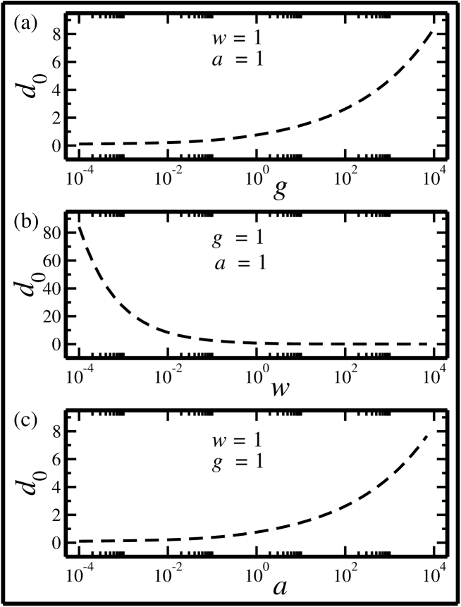
Figure 2: The correlation length, $d_{0}$, of the linear metabolic network versus the generation rate, $g$ (a); the degradation rate, $w$ (b); and the reaction rate, $a$ (c). High connectivity is reached when the primary process is the reaction process (proportional to $g$ and $a$). The correlation length $d_{0}$ decreases with increasing $w$ (as the degradation becomes dominant).

One can identify two limits. In the limit where $ag\gg w^{2}$ the correlations are strong, $q\rightarrow-1/2$ and $d_{0}\rightarrow\infty$. In this limit, the reaction process is dominant and long range correlations are observed. In the limit where $ag\ll w^{2}$, the correlations are weak, and $q\rightarrow 0$. In this limit the degradation process is dominant and the correlation length is small. In Fig. 2 we present the correlation length, $d_{0}$, as a function of the parameters $a$, $w$ and $g$ for a linear metabolic network. The correlation length increases with $a$ and $g$ (as the reaction process becomes dominant), and decreases with $w$ (as the process of degradation becomes dominant).

Using Eqs. (13) and (15), the connectivity $\eta$ can be expressed by $\eta=3d_{0}/J$. The linear network clearly demonstrates the difference between the concepts of TSW networks and FSW networks. In the topological sense it is as far as a network can be from a small world network, as the distance scales linearly with the network size, and the clustering coefficient is zero. However, in the functional sense the linear network can be a small world network, when the reaction terms are sufficiently dominant, enabling $d_{0}$ to become larger than $J$.

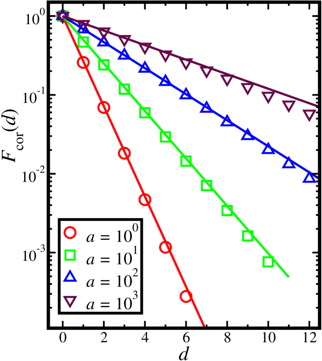
Figure 3: (color online) The correlation function $F_{\rm cor}(d)$ for the linear metabolic network as obtained from a numerical simulation for different values of the interaction rate $a$ (symbols). To conduct the numerical test we integrate the equations for the linear network and bring them to the steady state condition. Then we force a small perturbation $\Delta n_{0}$ on the concentration $n_{0}$ of the species $X_{0}$. We evaluate the correlation function using $F_{\rm cor}(d)=\left|\Delta n_{d}/\Delta n_{0}\right|$. The correlations decay exponentially with the distance between species. The typical correlation length increases as the reaction rate is increased. The results are in agreement with the theoretical results of Eq. (29) (solid lines). Slight deviations appear due to the fact that in numerical simulations $\Delta n_{0}$ must be finite.

In order to examine the theoretical predictions of the method, we conducted a simulation of the long linear metabolic network described above. In this simulation we constructed a linear network of $J=100$ reacting species with periodic boundary conditions, namely, $X_{0}$ reacts with $X_{99}$. At time $t=0$ we assigned to each reacting species its steady state concentration $n_{i}$. Then we forced the concentration $n_{0}$ to be slightly above its steady state value, namely $n_{0}(t)=n_{0}+\Delta n_{0}$, where $\Delta n_{0}\ll n_{0}$. We then let the network relax to its new steady state. We denote the resulting change in the steady state concentration of the species $X_{i}$ by $\Delta n_{i}$. In Fig. 3 we show the absolute value of $\Delta n_{i}/\Delta n_{0}$ as a function of $d$, the distance of the node $X_{i}$ from the perturbed node, $X_{0}$. These results, obtained from direct integration of the rate equations, are shown for different values of the reaction rate $a$ (symbols). When $a$ increases the typical correlation length becomes higher, and the effect of the local perturbation of $X_{0}$ extends to more distant species. The results are in good agreement with the theoretically derived correlation function, $F_{\rm cor}(d)$ [Eq. (29)] (solid lines). Slight deviations appear for distant species. This is because in numerical simulations one must choose $\Delta n_{0}$ to be a finite perturbation. The resulting deviation in the rest of the species is thus affected by higher order terms in the Taylor expansion which are not accounted for by our method. Here the generation rates and the degradation rates of all the species are $g=1$ and $w=1$ respectively. The network becomes an FSW network once $d_{0}\geq 17$, which is approximately the average path length for this network. This condition is satisfied for $a\geq 2\times 10^{5}$.

III.2 Perfect Tree Network

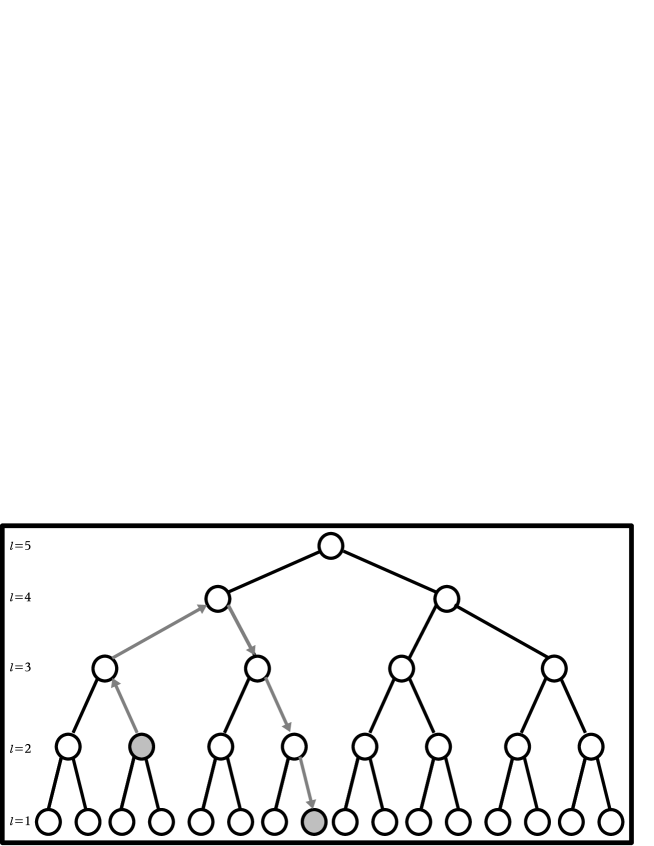
Figure 4: A tree-like network with $N=5$ levels. Each node is linked with exactly one node at the level above it (father), and $m$ nodes at the level below (siblings). The top node (here at level $l=5$) is the root node. The order of the tree is $m=2$, and the degree of the nodes is $r=3$. The path between a pair of nodes is characterized by the number of upward steps followed by the number of downward steps to get from one node to the other. For the path between the two shaded nodes $\vec{d}=(2,3)$.

Hierarchical structures are common in realistic networks. For instance, ecological networks have in many cases distinct trophic levels. Social organizations are also constructed in a tree-like framework. Here we relate to a hierarchical metabolic network. Consider a metabolic network of $J$ nodes where each node is assigned a level $l$ ($l=0,\dots,N$). The highest level $l=N$ consists of a single node, referred to as the root. Each node at level $l$ is then connected to exactly one node at level $l+1$ (the parent) and $m$ nodes at level $l-1$ (the siblings). The parameter $m$ is defined as the order of the tree. The degree of all the nodes (except those at the levels zero and $N$) is thus $r=m+1$ (Fig. 4). Since this network is hierarchical, the up and down directions are well defined. Stepping from a node at level $l$ to a node at level $l+1$ will be considered going up the network, while stepping from level $l$ to level $l-1$ is going down the network. Note that in a tree-like network it is not possible to go sideways, as there is no edge connecting two nodes at the same level. Consider a species $X_{i}$, which is at a distance $d$ from some other species $X_{j}$. The path between them consists of $u$ steps up the network and $v$ steps down the network. The total distance satisfies $d=u+v$, and the path between them can be noted by $\vec{d}=(u,v)$. For example, the path between the two shaded nodes in Fig. 4 is $\vec{d}=(2,3)$ and the distance is $d=5$. Two species are said to be located in the same branch if in the path between them either $u=0$ or $v=0$. The reaction rate matrix and the first order correlation matrix have non-zero values only for directly interacting species, namely, for pairs of species where either $u=1$ and $v=0$, or $v=1$ and $u=0$.

In order to avoid the complexities related to the boundaries of the network, we consider the case in which $N\gg 1$. For simplicity, we take the generation and the degradation rates to be $g_{i}=1$ and $d_{i}=1$ for $i=1,\dots,J$. The reaction rate is $a_{ij}=a$ for each pair of nodes $i$ and $j$ that react with each other. Under these conditions, the network is symmetrical and the rate equations are identical for all nodes:

$$\frac{dn}{dt}=1-n(t)-ran^{2}(t).$$ (31)

The steady state solution is thus

$$n=\frac{-1+\sqrt{1+4ra}}{2ra},$$ (32)

and the non-zero elements in the first order correlation matrix [Eqs. (4) and (5)] are

$$q=-\frac{4a}{\left(1+\sqrt{1+4ra}\right)^{2}}.$$ (33)

Two limits are observed. In the limit of strong interactions, where $a\gg 1$, the matrix elements approach $q\simeq-1/r$. In the limit of weak interactions, where $a\ll 1$ one obtains $q\simeq-a$. In any case the values that $q$ can take are limited to $-1/r\leq q\leq 0$.

For an infinite perfect tree with uniform rate constants, the correlation between all pairs of species with that same values of $u$ and $v$ are the same. We denote this correlation by $G_{u,v}$. In each line $i$ of the first order correlation matrix there are exactly $r$ non-zero terms. One term for $X_{i}$’s parent and $m$ terms corresponding to $X_{i}$’s siblings. The correlation $G_{u,v}$ between two species $X_{i}$ and $X_{j}$ is thus carried via the the parent of the species $X_{i}$, for which the correlation with $X_{j}$ is $G_{u-1,v}$, and via the $m$ siblings of the species $X_{i}$, for which the correlation with $X_{j}$ is $G_{u+1,v}$. Eq. (11) thus takes the form

$$\left\{\begin{array}[]{lrcr}G_{0,0}=1&&\\ G_{0,v}=q\left[G_{0,v+1}+G_{0,v-1}+(m-1)G_{1,v}\right]&&{\rm for}&v>0\\ G_{u,v}=q(G_{u-1,v}+mG_{u+1,v})&&{\rm for}&u>0\end{array}\right.$$ (37)

The first equation states that the correlation of every species with itself is unity. The second equation accounts for the correlations between species at the same branch, measuring the effect of variation in the higher level node on a node at a lower level. The third equation accounts for all the correlations that are not included in the first two equations. More specifically, it includes the correlations between species from different branches. It also includes the correlations between pairs on the same branch, measuring the effect of variation in the lower level node on a node at a higher level. We seek a solution of the form $G_{u,v}=e^{-\vec{k}\cdot\vec{d}}$, where $\vec{k}=(k_{1},k_{2})$ satisfies the condition that correlations vanish between distant species. From the third equation one obtains

$$k_{1}=\ln{\left[\frac{1}{2q}\left(1\pm\sqrt{1-4mq^{2}}\right)\right]},$$ (38)

while from the second equation one obtains

$$k_{2}=\ln{\left\{\frac{1}{2q}\left[\left(\frac{x-(m-1)q}{x}\right)\pm\sqrt{\left(\frac{x-(m-1)q}{x}\right)^{2}-4q^{2}}\right]\right\}},$$ (39)

where $x=e^{k_{1}}$. In order to satisfy the conditions that $G_{u,v}$ does not diverge for $u\gg 1$ while $-1/r\leq q\leq 0$, one has to choose the solution with the plus sign for $k_{1}$ in Eq. (38). The same condition for $v\gg 1$ requires one to choose the solution with the plus sign for $k_{2}$ in Eq. (39).

After some algebraic manipulations it can be shown that $k_{1}=k_{2}$. The correlation between any pair of species is thus

$$G_{u,v}=e^{i\pi d}e^{-\frac{d}{d_{0}}},$$ (40)

where $d=u+v$ is the distance between the two species, and

$$d_{0}=\left(\ln{\left|\frac{1+\sqrt{1-4mq^{2}}}{2q}\right|}\right)^{-1}$$ (41)

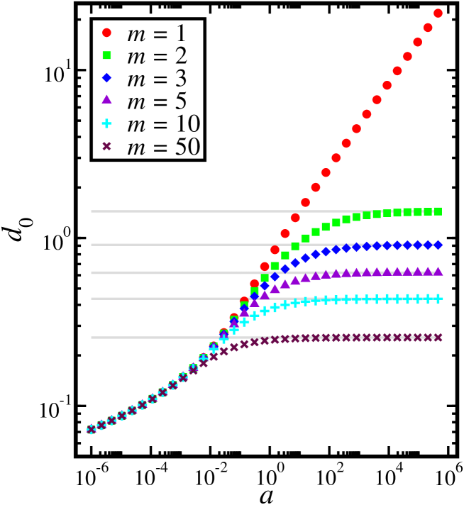
Figure 5: (color online) The correlation length $d_{0}$ versus the reaction rate $a$ for a metabolic network with a perfect tree structure. The results are shown for trees of different order, $m$ (symbols). For $m=1$ the results coincide with those obtained for the linear network. For higher orders the correlation length is bound from above by $d_{0}^{\rm max}=-1/\ln(m)$ (gray horizontal lines). Thus, for a sufficiently large tree-like network, where the average path length is larger than $d_{0}^{\rm max}$, the connectivity is always less than unity. Tree like networks are thus not expected to display FSW behavior.

is the correlation length of the tree-like network. The correlation function is $F_{\rm cor}(d)=\exp(-d/d_{0})$. Note that for $r=2$ ($m=1$) this solution coincides with the solution obtained for the linear network [Eq. (30)]. In the limit of weak interactions, where $a\ll 1$ and $q\rightarrow 0$ the correlation function approaches $F_{\rm cor}(d)\simeq|q|^{d}$. In this limit, due to the weak interactions, the correlation between a pair of species is dominated by the shortest path between them. In the limit of strong interactions, where $a\gg 1$ and $q\rightarrow-1/r$, the correlation length satisfies $d_{0}\rightarrow 1/\ln(m)$. For $m>1$ the correlation length is always finite. Since the average path length of a perfect tree-like network must scale in some form with the number of levels in the tree, one obtains that for a large enough tree network the connectivity will always be less than unity. Thus a perfect tree-like network of order $m=2$ or more will never be an FSW. In Fig. 5 we show the correlation length $d_{0}$ as obtained for a metabolic network with a perfect tree topology vs. the reaction rate $a$ (symbols). The results are shown for trees of different orders. Here $g=d=1$, and $a$ is varied.

IV More Complex Networks

To demonstrate the applicability of the NCF method, we now refer to the analysis of a set of more complex networks. Here analytical solutions are not available, and the correlation matrix must be obtained numerically. We analyze three different topologies following the structural classification proposed by Estrada Estrada2007 . The first example represents a class of networks which are organized into highly connected modules with few connections between them. The second example will be of a network with a highly connected central core surrounded by a sparser periphery, and the last example will be of a scale-free network.

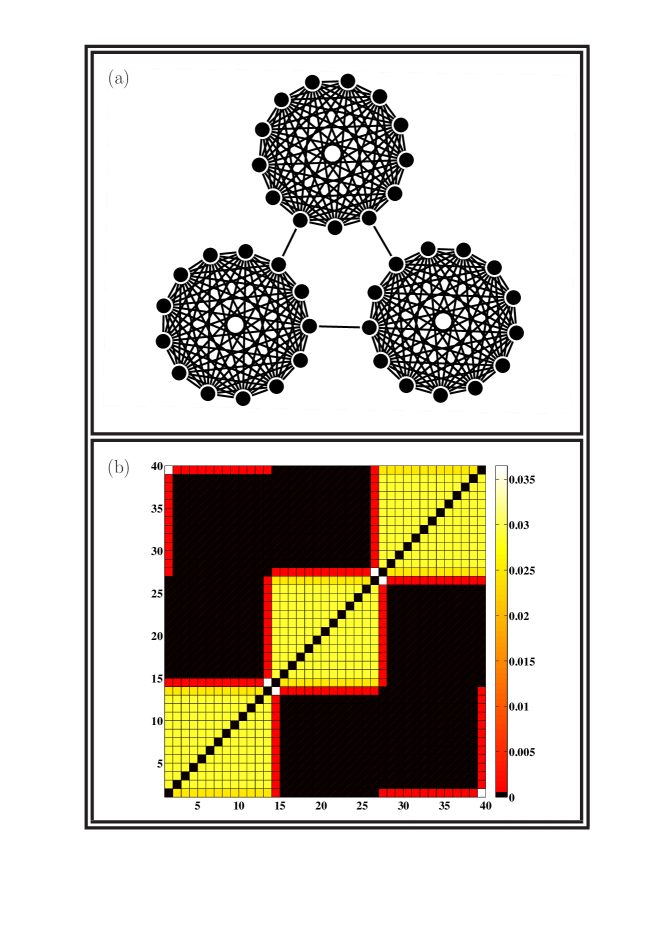
Figure 6: (color online) (a) A network constructed of three fully connected modules, with single bonds between them. (b) The correlation matrix features high correlations within the modules, and very small correlations between pairs of nodes from different modules. The matrix is constructed of three almost uncoupled blocks, reflecting the near bipartite topology of the network. The diagonal terms, which are all unity, do not appear in the Figure.

Consider a network constructed of three fully connected modules (communities), with a single connection between each pair of communities. This network is displayed in Fig. 6(a). Here, each community consists of $13$ nodes, adding up to a total of $J=39$ nodes. To obtain, $n_{i}$, $i=1,\dots,39$, the steady state solution for the concentrations of the different reacting species we solve Eq. (2) using a standard Runge-Kutta stepper. The parameters we use are $g_{i}=1$ and $d_{i}=1$. The reaction rate $a$ between pairs of reacting species is also set to unity. We then construct the first order correlation matrix, ${[}_{C]}ij$, as appears in Eq. (5). The complete correlation matrix, ${[}_{G]}ij$, is obtained from Eq. (11). It consists of a set of $39\times 39$ linear algebraic equations. Solving these equations, one obtains the complete correlation matrix of the network. For this network, the main insight on the global functions of the network can be deduced from the complete correlation matrix, which is displayed in Fig. 6(b). The diagonal terms, which are all unity, are omitted from the Figure. As expected, strong correlations appear between species within the same community (sub-matrices along the diagonal), and vanishingly small correlations appear between species from different communities. In fact, the correlation matrix is close to be a partitioned block matrix, except for a few coupling terms between the blocks. In this case the correlation matrix reflects the topological structure of the network, which is almost fully partitioned into three isolated communities.

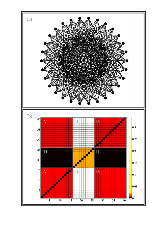
Figure 7: (color online) (a) A network consisting of a dense fully connected core with a sparse periphery. The peripheral nodes are each connected to all the central ones, but not to each other. (b) The correlation matrix shows strong correlations between pairs of species from the core (domain I). The strongest dependence is between nodes from the periphery to nodes from the core (domains II). However nodes from the core are almost not affected by nodes from the periphery (domains III). Interestingly, the correlations between pairs of nodes from the periphery are not so low, even though they are not directly connected to one another (domains IV). The diagonal terms, which are all unity, do not appear in the Figure.

We now consider a network, which features a highly connected central core surrounded by a sparser periphery. This network consists of $J=40$ nodes. The nodes $X_{i}$, $i=16,\dots,25$, are a fully connected cluster (the core), while the $30$ additional nodes are connected to all the nodes in the core, but not to each other (the periphery). This network is shown in Fig. 7(a). Following the same procedure described above one obtains the correlation matrix for this network [Fig. 7(b)]. The central square (domain I) shows the correlations between the nodes in the central core. Domains II show the correlations between peripheral nodes and central ones. The value of these correlations is high, expressing the strong dependence of the peripheral nodes on the nodes in the central core. On the other hand for the correlations between the central nodes and the peripheral ones (domains III) one obtains very low correlations. This is an expected result, as deviations in the population of a node from the periphery should have almost no effect on a node from the core. An interesting result appears in domains IV. These domains show the correlations between pairs of nodes that are both from the periphery. It turns out that the effect of these nodes on each other is stronger than the effect they have on their adjacent nodes from the core. This is even though the topological distance between peripheral nodes is $d=2$, while the distance between them and the central nodes is $d=1$. A small perturbation in a peripheral node results in a very minor effect on all the central nodes. However this minor change in the core results in a more dramatic effect on all the rest of the peripheral nodes. This non-trivial result exemplifies the importance of the functional methodology as a complimentary analysis to the common topological approach. In the two examples shown above, we focused on the insights provided by the complete correlation matrix. Below we show an additional numerical example, where we continue the analysis to obtain the correlation length, $d_{0}$, and the connectivity $\eta$.

One of the common characteristics of many realistic networks is their degree distribution that follows a power law, namely $P(k)=\alpha k^{-\lambda}$, where $\alpha$ and $\lambda$ are positive constants Barabasi1999 ; Albert2000 . Ecological networks, social networks and metabolic networks are characterized by power-law degree distributions, and are referred to as scale-free networks. Such networks include some nodes, called hubs, with a degree which is orders of magnitude higher than the average degree in the network. Scale free networks are considered as highly connected, because due to these hubs the average path length between nodes is small. In fact, in metabolic networks the average path length was found to be as small as $\langle[\rangle d]\simeq 3$ Jeong2000 . Below we examine a scale free network which is a TSW network, and determine whether it is also an FSW network.

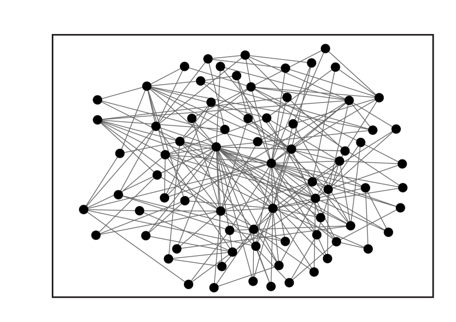
Figure 8: Scale free network consisting of 75 reacting species, constructed using the preferential attachment algorithm. The average path length of this network is $\langle[\rangle d]=2.43$ and its diameter is $D=4$.

To construct a scale free network we use the preferential attachment algorithm Barabasi1999 . In this algorithm a single new node is added at each iteration and $m$ edges are drawn from it to the set of existing nodes. The probability of linking the new node to some existing node $X_{i}$ is proportional to the current degree of the node $X_{i}$. This way, nodes which already have a higher degree than others have a high probability of obtaining more links and becoming hubs. Here we constructed a scale free network consisting of $J=75$ nodes. The number of edges added in each iteration was $m=3$. The result is the graph appearing in Fig. 8. The diameter of this network is $D=4$ and its average path length is $\langle[\rangle d]=2.43$.

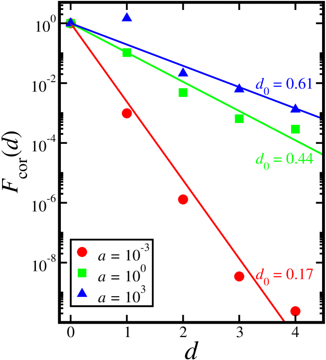
Figure 9: (color online) The correlation function vs. distance as obtained for the scale free network appearing in Fig. 8 for different values of the parameter $a$ (symbols). The correlations decay rapidly for low values of $a$, and more gradually for large values of $a$. By fitting the correlation function to an exponential (solid lines), the correlation length $d_{0}$ can be obtained.

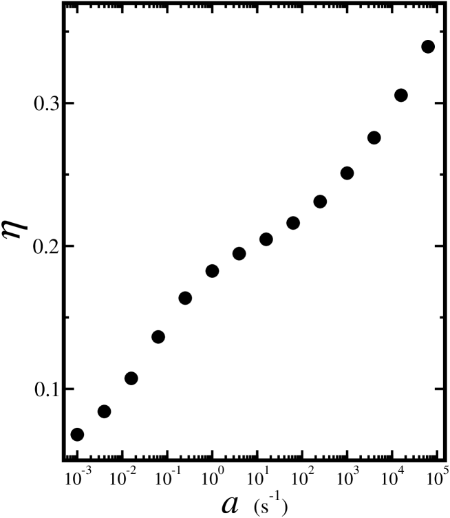
Figure 10: The connectivity, $\eta$ vs. $a$ as obtained for the scale free network shown in Fig. 8. The connectivity increases logarithmically as a function of $a$. Note that $\eta<1$ for a very broad range of values of the parameter $a$. This implies that although scale-free networks are commonly TSW networks, in the functional sense they may not be FSW networks.

Solving Eq. (2) we obtain the steady state solution for the concentrations of all the reactive species. The parameters are $g_{i}=1$ and $d_{i}=1$ for $i=1,\dots,75$. The reaction rate $a$ between pairs of reacting species is varied. In this case, obtaining the complete correlation matrix, ${[}_{G]}ij$, requires the solution of $75\times 75$ linear algebraic equations [Eq. (11)]. We solve these equations and then average over the correlations between equidistant species to obtain the correlation function $F_{\rm cor}(d)$ [Eq. (12)]. In Fig. 9 we show the resulting correlation function $F_{\rm cor}(d)$ vs. $d$ for three different values of the reaction rate $a$ (symbols). When the interaction is suppressed ($a\ll 1$) the correlations decay rapidly. When the interaction is dominant ($a\gg 1$), correlations are maintained over long distances. By fitting the correlation functions to exponential functions (solid lines) one obtains the typical correlation length, $d_{0}$, and the connectivity, $\eta$, of each of the networks. The results for $\eta$ vs. the reaction rate $a$ are shown in Fig. 10. It is found that the connectivity increases logarithmically with $a$. Note that for a very wide range of values of the parameter $a$, the connectivity remains lower than unity. This means that although the examined scale free network is a TSW, for a very wide range of parameters it is not an FSW. Only in the extreme cases of very strong interactions FSW behavior might emerge.

V Summary and Discussion

We have presented the NCF method for the analysis and evaluation of the connectivity of interaction networks. The method complements the topological analysis of networks, taking into account the functional nature of the interactions and their strengths. The method enables to obtain the correlation matrix, which provides the correlations between pairs of directly and indirectly interacting nodes. In certain cases, one may gain insights on the network’s functionality by writing down the complete correlation matrix. For instance, one can identify domains of high and low correlations. In other cases it is more insightful to extract the macroscopic characteristics of the network from the matrix. In particular, we have shown how to calculate the typical correlation length of the network. This correlation length, which has to do with the functionality of the network, can be compared to topological characteristics such as the average minimum path length of the network. The ratio between these two lengths provides the characteristic connectivity of the network. It was shown that the topological analysis alone is not sufficient in order to characterize the functionality of a network. For instance, networks with small world topology may display low connectivity, while networks that do not exhibit small world topology may display high connectivity. This is because in terms of the functionality of the network, when the correlation length is large, even distant species may be highly correlated. We demonstrated the method for metabolic networks with different topological structures, and identified the regimes of low connectivity and of high connectivity. As expected, these regimes depend on topological features, such as the number of species or the average minimum path length between pairs of species. However, they also depend on functional features such as the type of interactions in the network and the rate constants of the different processes.

The NCF method was demonstrated for metabolic networks, but its applicability is much wider. In fact, the method could be applied to any reaction network that can be modeled by rate equations. Such networks include metabolic networks Peacocke1989 , chemical networks Tielens2005 ; Gillespie2007 , gene expression networks Palsson2006 ; Alon2006 and ecological networks Murray1989 . It is common to use rate equations for the modeling of these types of networks. In certain models of social networks, the flow of information as well as the spreading of viruses can also be described by rate equations. The method is not suitable for obtaining the correlations in Ising type models, where the nodes are assigned discrete variables, which cannot be modeled using continuous equations. The number of elements in the correlation matrix is equal to the number of pairs of nodes in the system. When applying the NCF method, one writes a single linear equation for each matrix element. Thus, from a computational point of view, the scaling of the NCF method is quadratic in the number of reactive species. This enables the application of the method to networks which include even thousands of nodes. It is straightforward to extend the application of the method to the other types of interaction networks mentioned above. A few examples are addressed below.

Consider, for example, gene expression networks. These networks consist of genes and proteins that interact with each other. In addition to protein-protein interactions, already analyzed in the context of metabolic networks, genetic networks include transcriptional regulation processes, where some genes regulate the expression of other genes. In recent years, much information has been acquired about the topology of these networks, for certain organisms such as Escherichia coli Alon2006 . The problem is that these networks are very elaborate, and may consist of thousands of nodes. This limits our ability to simulate their functionality, and thus, currently most of the theoretical and computational analysis of these networks is focused on small modules Alon2006 . In this analysis, one performs simulations of small subnetworks consisting of only a few nodes. These subnetworks are expected to play specific roles in the functionality of the network as a whole. Such approach is valid if an isolated module maintains its function when incorporated in a large network in which it interacts with many other genes. We expect the analysis presented here to provide some insight on this matter. By obtaining the complete correlation matrix, one can characterize the dependence of different proteins and genes on one another. The network may then be divided into subnetworks, grouping together nodes that are highly correlated, and excluding ones that are not. It is expected that these modules will not function significantly differently when analyzed in the context of the surrounding network nodes. In addition, the typical correlation length will provide us with an approximate radius beyond which correlations may be neglected. To simulate a module properly, one needs to include all the nodes which are within that radius from the module. Other possible applications regard social networks. For instance, the process of viral spreading could be analyzed PastorSatorras2001 ; Lind2007 . Many social networks are known to be small world networks. However, this does not mean that any contagious disease spreads rapidly. This is, possibly, because for certain diseases the correlation length is small. Using the method presented here, one can obtain this correlation length, taking into account the specific rate constants of the viral flow.

The recent applications of graph theory to many natural macroscopic systems was enabled by focusing on their topology. This approach has been very fruitful, as it uncovered the mutual structure of networks from many different fields. In particular, the ubiquity of the scale free degree distribution, and the small world topology was found. However, it still is not completely clear what functional meaning can be given to these topological properties in different contexts. A recently proposed approach derives the key aspects of the network functionality from its topological structure Stelling2002 . Other approaches use the Ising Hamiltonian to describe the interaction pattern between nodes on scale free and small world networks Jeong2003 ; Pekalski2001 . Functional characteristics such as phase transitions, and critical exponents are then observed. The NCF method presented in this paper complements these approaches. It can be applied to a variety of different interaction processes, such as metabolic, ecological or social interactions, all of which can be described by rate equations. We believe that the approach presented here will lead to new insights on the behavior of networks and their functionality.

Figure 1: The linear metabolic network. Each molecular species $X_{i}$ reacts with its two nearest neighbors, $X_{i-1}$ and $X_{i+1}$.

References

- (1) D. J. Watts and S. H. Strogatz, Nature 393, 440 (1998).
- (2) S. Wasserman and K. Faust, Social Network Analysis Methods and Applications (Cambridge University, Cambridge, 1994).
- (3) A. Barrat and M. Weigt, Eur. Phys. J. B 13, 547 (2000).
- (4) M. E. J. Newman, J. Stat. Phys. 101, 819 (2000).
- (5) P. Erdös and Rényi, Publ. Math. 6, 290 (1959).
- (6) P. Erdös and Rényi, Publ. Math. Inst. Hung. Acad. Sci. 5, 17 (1960).
- (7) P. Erdös and Rényi, Bull. Inst. Int. Stat. 38, 343 (1961).
- (8) F. Chung and L. Lu, Adv. Appl. Math. 26, 257 (2001).
- (9) A. L. Barabási, H. Jeong, E. Ravasz, Z. Néda, A. Schubert and T. Vicsek, Physica A 311, 590 (2002).
- (10) M. Kochen, 1989, The Small World (Albex, Norwood, New Jersey, 1989).
- (11) M. E. J. Newman, Proc. Natl. Acad. Sci. U.S.A. 98, 404 (2001).
- (12) M. E. J. Newman, Phys. Rev. E 64, 016131 (2001).
- (13) M. E. J. Newman, Phys. Rev. E 64, 016132 (2001).
- (14) S. Redner, Eur. Phys. J. B 4, 131 (1998).
- (15) A. Vázquez, Statistics of Citation Networks, preprint cond-mat/0105031.
- (16) A. L. Barabási and R. Albert, Science 286, 509 (1999).
- (17) R. Albert, H. Jeong and A. L. Barabási, Nature 406, 378 (2000).
- (18) L. A. N. Amaral A. Scala, M. Barthélémy and H. E. Stanley, Proc. Natl. Acad. Sci. U.S.A. 97, 11149 (2000).
- (19) S. Lawrence and C. L. Giles, Science 280, 98 (1998).
- (20) S. Lawrence and C. L. Giles, Nature 400, 107 (1999).
- (21) R. Albert, H. Jeong and A. L. Barabási, Nature 401, 130 (1999).
- (22) A. Broder, R. Kumar, F. Maghoul, P. Raghavan, S. Rajalopagan, R. Stata, A. Tomkins and J. Wiener, Comput. Netw. 33, 309 (2000).
- (23) L. A. Adamic and B. A. Huberman, Science 287, 2115 (2000).
- (24) L. A. Adamic, in Proceedings of the Third European Conferene, ECDL’99, edited by G. Goos, J. Hartmanis and J. van Leeuwen (Springer-Verlag, Berlin, 1999), p. 433.
- (25) S. L. Pimm, The Balance of Nature (University of Chicago, Chicago, 1991).
- (26) R. J. Williams, N. D. Martinez, E. L. Berlow, J. A. Dunne and A. L. Barabási, Proc. Nat. Acad. Sci. US 99, 12913 (2002).
- (27) J. M. Montoya and R. V. Solé, J. Theor. Biol. 214, 405 (2002).
- (28) J. Camacho, R. Guimerá and L. A. N. Amaral, Phys. Rev. Lett. 88, 228102 (2002).
- (29) A. Wagner and D. Fell, Proc. Roy. Soc. London Series B, 268, 1803 (2001).
- (30) D. A. Fell and A. Wagner, Nat. Biotechnol. 18, 1121 (2000).
- (31) H. Jeong, B. Tombor, R. Albert, Z. N. Oltvai and A. L. Barabási, Nature 407, 651 (2000).
- (32) R. Albert and A. L. Barabási, Rev. Mod. Phys. 74, 47 (2002).
- (33) E. Estrada, Phys. Rev. E 75, 016103 (2007).
- (34) A. R. Peacocke, An Introduction to the Physical Chemistry of Biological Organization (Oxford Science Publications, Oxford, 1989)
- (35) A.G.G.M. Tielens, The Physics and Chemistry of the Interstellar Medium (Cambridge University Press, Cambridge, 2005).
- (36) D.T. Gillespie, Annu. Rev. Phys. Chem. 58, 35 (2007).
- (37) B.O. Palsson, Systems Biology: Properties of Reconstructed Networks (Cambridge University Press, Cambridge, 2006).
- (38) U. Alon, An introduction to systems biology: design principles of biol ogical circuits (Chapman & Hall/CRC, London, 2006).
- (39) J.D. Murray, Mathematical Biology (Springer, Berlin, 1989).
- (40) P.G. Lind, L.R. da Silva, J.S. Andrade Jr. and H.J. Herrmann, Phys. Rev. E 76, 036117 (2007).
- (41) R. Pastor-Satorras, A. Vázquez and A. Vespignani, Phys. Rev. Lett. 87, 258701 (2001).
- (42) J. Stelling, S. Klamt, K. Bettenbrock, S. Schuster and E.D. Gilles, Nature 420, 190 (2002).
- (43) D. Jeong, H. Hong, B.J. Kim and M.Y. Choi, Phys. Rev. E 68, 027101 (2003).
- (44) A. Pekalski, Phys. Rev. E 64, 057104 (2001).