Nonassociative quantum theory, emergent probability, and coquasigroup symmetry

Abstract.

This paper follows recent steps towards a nonassociative quantum theory and points out the mathematical structure behind the proposed modifications to conventional quantum theory. An $N=1$ supersymmetry model and a strong force glueball ansatz is highlighted. Using nonassociative complex octonion algebra, it is shown how the Lorentz Lie algebra can be understood as a four dimensional generalization of the algebra of spin-1/2 operators in physics. Probability is speculated to become an emergent phenomenon from some nonassociative geometry in which to better understand the fluxes involved. A prototype nonassociative quantum theory in one dimension is brought forward to illustrate how normed division algebras may aid in modeling isospin properties that are similar to observed field and particle symmetries in nature. This prototype is built from a principle of self-duality between types of active and passive transformations and supplied with a modified Born rule that models observation, similar to conventional quantum mechanics. Solutions on the complex numbers, quaternions and octonions are discussed. The Hopf coquasigroup structure of the octonionic eigenvalue relation is shown and advertised as a tool for future investigation into the complete solution set of the model.

1. Introduction

A primary motivation for work towards a complete, consistent quantum theory on nonassociative spaces is the desire to model more physical forces with fewer assumptions. Theoretical reductionism is particularly important when the consequences of a proposed model are hard or impossible to measure, as is the case in quantum gravity. How can one unification proposal be evaluated against another? Today’s description of physical law does not require nonassociativity as a fundamental notion in quantum mechanics. On the other hand, it is unclear whether quantum gravity and its unification with the Standard Model may ever be modeled using conventional associative geometry.

If nonassociativity is a fundamental property of nature, as presumed here, then it must be shown how today’s conventional formulations may emerge from such foundation without contradicting the observation. Section 2 follows up on recent investigations into nonassociative quantum theory and highlights the mathematical structure of certain modifications to conventional quantum theory: Nonassociative parts of quantum mechanical operators are unobservable in principle[8], and decompositions exist for a supersymmetric nonrelativistic Hamiltonian[9], the spin-$\frac{1}{2}$ operator algebra and Lorentz Lie algebra[11, 27], and the hypothesized “glueball” particle from strongly interacting fields[12, 13, 14]. It is shown how probability conservation in conventional quantum mechanics may become an emergent phenomenon that may be better described in a nonassociative geometry to be found.

There are many proposals today that introduce nonassociativity into conventional quantum formulations. More direct approaches may use nonassociative algebras, such as the octonions or split-octonions, instead of customary complex number or matrix algebra. More indirect approaches embed observed Lie group symmetries into the exceptional Lie groups, which are automorphism groups of types of nonassociative algebras (for a review see e.g. [2]). The range of envisioned applications spans much of fundamental physics. A certainly incomplete list of nonassociativity in quantum physics over the past four decades includes: quark statistics in the Strong Force[20, 21, 22, 35], chirality and triality in fundamental particles[37], Standard Model symmetries from spinors over the division algebras [5, 15], the Weak Force and Yang-Mills instantons[35], octonionic quantum theory and Dirac equation from left/right-associating operators [29, 30, 31], fermion generations[6, 33], a geometric relation between Heisenberg uncertainty and the light cone[16], the Dirac equation with electromagnetic field[17, 18, 26], a four dimensional Euclidean operator quantum gravity[25, 27], Lie group symmetries of the Standard Model [7, 34] with gravity[32], and supersymmetry with the Standard Model[3, 4]. These and other approaches introduce nonassociativity into existing formulations in physics, which requires modifying some assumptions while keeping others unchanged. Yet, with all these clues and hints it is entirely in the open whether a “better” description of physical law may ever be found this way. If one believes this could be accomplished, the tantalizing question is: Which, and how many, of today’s paradigms in physics need to be amended?

Section 3 proposes a new prototype nonassociative quantum theory in one dimension that is built from algebraic and geometric rules. Rather than declaring physical principles up front (e.g. conservation of probability, invariance of the speed of light, equivalence of energy and masses), the model builds wave functions from self-dual types of transformations. The Born rule which governs observation in conventional quantum mechanics is modified, and requires the operator/eigenfunction/eigenvalue relation to be contained in a complex number subalgebra of the otherwise quaternionic or octonionic formulation. Solutions exist that are similar to what one could expect from a physical model.

All work is done under the speculation that the prototype’s current limitation of one spacial dimension may eventually be overcome and model nature’s spacetime as we observe it. One possible way towards achieving this goal is shown in section 4. A further generalized Born rule requires the real eigenvalue of the operator/eigenfunction relation to remain invariant under changes between equivalent algebras. An understanding of the complete solution set of such a generalization appears contingent on a proper mathematical tool. The eigenvalue equations to be solved are shown to have Hopf coquasigroup structure [23].

2. Towards a nonassociative quantum theory

Conventional operator quantum mechanics uses unobservable wave functions $\Psi$ that are decomposed into orthogonal eigenfunctions $\psi_{n}$ of an operator $H$, to yield observable eigenvalues $h_{n}$. The expectation value of $H$ over some configuration space $V$ is then determined through expressions like:

$$\left\langle\Psi\right|H\left|\Psi\right\rangle =\sum_{n}h_{n}\int_{V}\psi_{n}^{*}\psi_{n}dV.$$

Probability density $\rho$ models the relative frequency of occurrence of measurement outcomes $h_{n}$, and is defined through:

$$\rho :=\left\langle\Psi\right|1\left|\Psi\right\rangle=\sum_{n}\rho_{n}, \rho_{n} :=\int_{V}\psi_{n}^{*}\psi_{n}dV.$$

What is also called the “Born rule” gives the expectation value of $H$ as:

(2.1) $$\left\langle\Psi\right|H\left|\Psi\right\rangle =\sum_{n}h_{n}\rho_{n}.$$

As a special case, the Hamiltonian operator of a quantum mechanical system allows to describe the time dependency of other operators through Ehrenfest’s theorem. If $H$ is the Hamiltonian and $L$ another operator on that same system, then the expectation value of $L$ as a function of time is:

(2.2) $$\left\langle\Psi\right|\frac{dL}{dt}\left|\Psi\right\rangle =\left\langle\Psi\right|\frac{\partial L}{\partial t}+\frac{\imath}{\hbar}\left[H,L\right]\left|\Psi\right\rangle.$$

Here, $\imath$ is the imaginary basis element of the complex numbers, $b_{\mathbb{C}}=\left\{1,\imath\right\}$.

Two operators $H_{1},H_{2}$ with eigenvalues $h_{1n},h_{2n}$ model physical quantities that can be observed simultaneously only if they commute:

$$H_{1}\left(H_{2}\left|\Psi\right\rangle\right)=H_{2}\left(H_{1}\left|\Psi\right\rangle\right) \Longleftrightarrow h_{1n}\textrm{ and }h_{2n}\textrm{ simultaneously observable}.$$

For example, momentum operator $\hat{p}_{i}:=-\imath\hbar\partial/\partial x_{i}$ (with $i=1,2,3$) and angular momentum operator $\hat{L}_{i}:=-\imath\hbar\left(\vec{x}\times\nabla\right)_{i}$ allow only components with same index $i$ to be measured simultaneously since $\hat{p}_{i}\left(\hat{L}_{i}\left|\Psi\right\rangle\right)=\hat{L}_{i}\left(\hat{p}_{i}\left|\Psi\right\rangle\right)$, but not two different components since generally $\hat{p}_{i}\left(\hat{L}_{j}\left|\Psi\right\rangle\right)\neq\hat{L}_{j}\left(\hat{p}_{i}\left|\Psi\right\rangle\right)$ for $j\neq i$.

2.1. Nonassociativity and unobservables

Noncommutativity of operators from conventional quantum mechanics is now extended to nonassociativity and speculated to be of use in a future nonassociative quantum theory. New kinds of operators $Q_{n}$ may in general not satisfy:

(2.3) $$\left\langle\Psi\right|\left(Q_{n}\left|\Psi\right\rangle\right) \neq\left(\left\langle\Psi\right|Q_{n}\right)\left|\Psi\right\rangle.$$

This requires additional rules to be supplied to the Ehrenfest theorem (2.2) or the Born rule (2.1), to obtain expectation values of the $Q_{n}$, understand their evolution over time and predict measurement outcomes unambiguously.

This can be realized by having $Q_{n}$ and the $\left|\Psi\right\rangle$ in some nonassociative algebra. Such operators are interpreted to model “unobservables” that cannot be measured in principle [8]. The concept is distinct from conventional “hidden variables” models, which contain information that could in principle be extracted from the quantum system. An example of an unobservable property in nature would be the color charge in the Strong Force, a property that is instrumental in the workings of the force; however, cannot be observed from the outside. It is pointed out that unobservables do not need to be quantum contributions on small scales. They may in general be of the same order of magnitude as conventional observable properties.

There are many ways of bringing this general approach into agreement with the observation. One way is to decompose known operators into unobservable parts, define dynamics of these parts and show how the conventional formulation emerges in the appropriate limit. For example, if $H$ is an operator from conventional quantum mechanics, it could be made from parts, $H:=Q_{1}Q_{2}$, where the $Q_{1}$ and $Q_{2}$ are unobservables. A nonassociative quantum theory, to be found, would then have to explain why such decomposition is necessary or desirable, as opposed to merely being possible.

To give an example, without going into the model assumptions, a Hamiltonian $H$ is proposed in [9, 11] to be made from $Q_{1}$ and $Q_{2}$ with the following properties:

$$H := \frac{1}{2}\left(Q_{1}+Q_{2}\right)^{2},$$

$$Q_{1}Q_{1}\left|\Psi\right\rangle=Q_{2}Q_{2}\left|\Psi\right\rangle = 0,$$

$$\left(Q_{1}Q_{2}\right)\left|\Psi\right\rangle = \left(Q_{2}Q_{1}\right)\left|\Psi\right\rangle,$$

$$\left\langle\Psi\right|\left(Q_{n}\left|\Psi\right\rangle\right) \neq \left(\left\langle\Psi\right|Q_{n}\right)\left|\Psi\right\rangle\qquad\left(n\in\left\{1,2\right\}\right),$$

$$\left\langle\Psi\right|\left(\left(Q_{1}Q_{2}\right)\left|\Psi\right\rangle\right) = \left(\left\langle\Psi\right|\left(Q_{1}Q_{2}\right)\right)\left|\Psi\right\rangle.$$

The $Q_{1}$ and $Q_{2}$ are unobservables per (2.3). These relations can be satisfied when modeling the $Q_{1/2}$ as linear differential operators and using nonassociative split-octonion algebra (for details, see [9, 11]). A new quantum theory could then specify the dynamics of $Q_{1/2}$ and split-octonion wave functions $\left|\Psi\right\rangle$, but model the observable operator $H=Q_{1}Q_{2}=Q_{2}Q_{1}$ in agreement with conventional quantum theory.

2.2. Example: Spin operator and Lorentz Lie algebra from nonassociative algebra

For a new nonassociative quantum theory to be useful or desired, it has to do more than just recreating known physics. There have to be novel observable effects, or it has to describe known effects using fewer assumptions. This section gives an example that hints towards the latter. A nonassociative algebra is shown to have two associative subalgebras, each of which models an independent effect in physics: the algebra of spin operators from spin-$\frac{1}{2}$ particles, and the Lorentz Lie algebra from Special Relativity [10]. The finding demonstrates an opportunity for a future quantum theory that uses nonassociative algebra, to let previously unrelated descriptions of natural law emerge from a single formalism.

Algebra of spin-$\frac{1}{2}$ operators

A spin in physics is a fundamental internal property of particles or bound quantum systems, such as atomic nuclei. It is independent from the space-time or energy-momentum parameters that describe other dynamic properties. A simple example is a spin-$\frac{1}{2}$ particle, where two spin states are possible when measured along any direction in space: “up” or “down”. Conventional quantum mechanics describes spin observables through operators $\hat{s}_{j}$:

$$\hat{s}_{j} :=\frac{1}{2}\sigma_{j}\qquad\left(j\in\left\{1,2,3\right\}\right).$$

The index $j$ enumerates three orthogonal spacial axes $x_{j}$ along which to measure. In the choice of units here, only a factor $\frac{1}{2}$ comes with the $\sigma_{j}$, which are the Pauli matrices over complex numbers. To basis $b_{\mathbb{C}}=\left\{1,\imath\right\}$ these are:

(2.10) $$\sigma_{1} :=\left(\begin{array}[]{rr}0&1\\ 1&0\end{array}\right), \sigma_{2} :=\left(\begin{array}[]{rr}0&-\imath\\ \imath&0\end{array}\right), \sigma_{3} :=\left(\begin{array}[]{rr}1&0\\ 0&-1\end{array}\right),$$

(2.13) $$\sigma_{j}\sigma_{j} =\left(\begin{array}[]{rr}1&0\\ 0&1\end{array}\right)=\left(\mathrm{id}\right), \sigma_{j}\sigma_{k} =-\frac{\imath}{2}\sum_{l=1}^{3}\epsilon_{jkl}\sigma_{l} \left(j,k\in\left\{1,2,3\right\}\right).$$

Born’s rule gives measurable spin states from eigenfunctions $\left|\Psi\right\rangle$ to the $\sigma_{j}$, so that $\sigma_{j}\left|\Psi\right\rangle=\lambda\left|\Psi\right\rangle$ with real eigenvalues $\lambda=+\frac{1}{2}$ for “spin up” and $\lambda=-\frac{1}{2}$ for “spin down” along an axis of measurement.

Without addressing physical measurement, the algebra of $\sigma_{j}$ operators (2.10) can be expressed in the associative complex quaternion algebra. Written to a quaternion basis $b_{\mathbb{H}}=\left\{1,i_{1},i_{2},i_{3}\right\}$ and complex number coefficients to $b_{\mathbb{C}}=\left\{1,\imath\right\}$, the $\sigma_{j}$ can be defined as:

(2.14) $$\sigma_{j} :=\imath i_{j}.$$

On a side note, the imaginary quaternions (here to basis elements $\left\{i_{1},i_{2},i_{3}\right\}$) also generate the $\mathfrak{su}\left(2\right)$ Lie algebra.

Lorentz Lie algebra

The Lorentz group is the matrix Lie group that preserves the quadratic form $\left|\cdot\right|$ on four-vectors $x:=\left(x_{0},x_{1},x_{2},x_{3}\right)$:

$$\left|\cdot\right| \,:\,\mathbb{R}^{4}\rightarrow\mathbb{R}, \left|x\right| :=x_{0}^{2}-x_{1}^{2}-x_{2}^{2}-x_{3}^{2}=x_{0}^{2}-\left\|\vec{x}\right\|^{2}.$$

In Special Relativity in physics, this quadratic form is interpreted as the metric tensor $\eta$ of Minkowski spacetime:

$$\eta_{\mu\nu} :=\left(\begin{array}[]{rrrr}1&0&0&0\\ 0&-1&0&0\\ 0&0&-1&0\\ 0&0&0&-1\end{array}\right), \left|x\right| =\sum_{\mu,\nu=0}^{3}x_{\mu}x_{\nu}\eta_{\mu\nu}.$$

Here, $x_{0}$ is called the “time component” and $\vec{x}:=\left(x_{1},x_{2},x_{3}\right)$ the “spacial components” of the four-vector $x$. Examples for such four-vectors are energy-momentum $p:=\left(E,p_{1},p_{2},p_{3}\right)=\left(E,\vec{p}\right)$ or space-time intervals $dx:=\left(dt,dx_{1},dx_{2},dx_{3}\right)=\left(dx_{0},d\vec{x}\right)$. The preserved quadratic form of energy-momentum corresponds to invariant mass $m^{2}=E^{2}-\left\|\vec{p}\right\|^{2}$, and space-time intervals model invariant proper time $d\tau^{2}=dt^{2}-\left\|d\vec{x}\right\|^{2}$.

These physical properties remain unchanged when translating between equivalent frames of reference. Next to a translation symmetry, the geometry of Minkowski spacetime is symmetric under rotation in space, and transformations between uniformly moving, nonaccelerated frames of reference. The last two symmetries together make up the Lorentz group. The associated Lie algebra of the generators of Lorentz transformation $M_{\mu\nu}$ is:

(2.15) $$\left[M_{\mu\nu},M_{\rho\sigma}\right] =\imath\left(\eta_{\nu\rho}M_{\mu\sigma}+\eta_{\mu\sigma}M_{\nu\rho}-\eta_{\mu\rho}M_{\nu\sigma}-\eta_{\nu\sigma}M_{\mu\rho}\right),$$

$$x_{\mu}^{\prime} :=\sum_{\mu=0}^{3}M_{\mu\nu}x_{\nu},\qquad\mu,\nu,\rho,\sigma\in\left\{0,1,2,3\right\}.$$

The $M_{\mu\nu}$ rotate the spacial components of a four-vector $x$, and perform so-called “Lorentz boosts”.

Similar to the algebra of spin-$\frac{1}{2}$ operators above, the Lorentz Lie algebra can be generated with octonions $\mathbb{C}\otimes\mathbb{O}$ to basis $\left\{1,\imath\right\}\otimes\left\{1,i_{1},\ldots,i_{7}\right\}$ when defining [10, 27]:

$$R_{0} :=\frac{i_{4}}{2}\left(1+\imath\right), R_{j} :=\frac{i_{\left(j+4\right)}}{2}\left(1-\imath\right), \left(j\in\left\{1,2,3\right\}\right)$$

$$M_{\mu\nu} :=\frac{1}{2}\left[R_{\mu},R_{\nu}\right].$$

All terms of the $M_{\mu\nu}$ are calculated in appendix A, and it follows directly that the defining relation of the Lorentz Lie algebra (2.15) is satisfied.

Nonassociative algebra

The spin-$\frac{1}{2}$ operator generated by $\sigma_{j}$ (2.14) and the Lorentz Lie algebra generated by $M_{\mu\nu}$ (2.15) are both expressed on complex octonions:

$$\sigma_{j} :=-\frac{\imath}{4}\epsilon_{jkl}R_{k}R_{l}, M_{\mu\nu} :=\frac{1}{2}\left[R_{\mu},R_{\nu}\right].$$

The four $R_{\mu}$ satisfy the additional associator relation:

$$\left(R_{\mu},R_{\nu},R_{\rho}\right) :=\left(R_{\mu}R_{\nu}\right)R_{\rho}-R_{\mu}\left(R_{\nu}R_{\rho}\right)=2\sum_{\sigma,\xi=0}^{3}\epsilon_{\mu\nu\rho\xi}\eta_{\xi\sigma}R_{\sigma}.$$

One can validate this expression from

$$\left(i_{\mu},i_{\nu},i_{\rho}\right) =2\sum_{\sigma=4}^{7}\varepsilon_{\mu\nu\rho\sigma}i_{\sigma}, \mu,\nu,\rho \in\left\{4,5,6,7\right\},$$

which is a property of any antiassociative four-tuple in the octonions (here: $\left\{i_{4},i_{5},i_{6},i_{7}\right\}$). The Minkowski tensor $\eta_{\xi\sigma}$ then comes from the difference in sign in the $\left(1\pm\imath\right)$ factor of $R_{0}$ and the $R_{j}$.

With this, the four element set $\left\{R_{0},R_{1},R_{2},R_{3}\right\}$ that generates the Lorentz Lie algebra can be viewed as a four dimensional “spacetime” generalization of the $\left\{R_{1},R_{2},R_{3}\right\}$ set that generates the algebra of spin-$\frac{1}{2}$ operators, $\sigma_{j}$, in three dimensional space.

2.3. Example: Operator algebra of strongly interacting fields and glueball

The Strong Force in physics is the interaction between building blocks of matter, the quarks. It is mediated through exchange particles, the gluons. Both quarks and gluons carry a color charge, but neither charges nor particles can be isolated or directly observed. This is known as color confinement in physics.

In the context of this paper, this means that there exist no operators $A$ in conventional quantum mechanics that would allow measurement of the color charge with real eigenvalues $a_{n}$ after the Born rule (2.1) to $\left\langle\Psi\right|A\left|\Psi\right\rangle=\sum_{n}a_{n}\rho_{n}$. This section shows how a certain modification to this rule for observation in quantum mechanics makes room for nonassociative operator algebras. This may aid in modeling the glueball, a hypothetical particle that is made from gluons only [13, 14].

Observables from nonassociative parts of an operator and modified Born rule

A product of two operators $A^{B}$ and $A^{C}$ is measured in conventional quantum mechanics as:

$$A^{B}A^{C}\left|\Psi\right\rangle \overset{\mathrm{def}}{=}A^{B}\left(A^{C}\left|\Psi\right\rangle\right).$$

The operators $A^{B},A^{C}$ are now proposed to be made from a product of operators $e$, $\Phi^{B}$ and $\Phi^{C}$:

$$A^{B} :=e\Phi^{B}, A^{C} :=e\Phi^{C}.$$

The operator algebra $\mathbb{G}$ of the $A^{B}$ and $A^{C}$ is associative by definition, whereas the $e$, $\Phi^{B}$ and $\Phi^{C}$ are elements in a nonassociative operator algebra $\mathbb{A}$:

$$A^{B},A^{C} \in\mathbb{G}, e,\Phi^{B},\Phi^{C} \in\mathbb{A}.$$

A modification to the Born rule for observability in quantum mechanics can then be proposed. For operators that are made from nonassociative parts, measurement requires to reassociate the parts:

$$A^{B}A^{C}\left|\Psi\right\rangle =A^{B}\left(A^{C}\left|\Psi\right\rangle\right)=\left(e\Phi^{B}\right)\left(\left(e\Phi^{C}\right)\left|\Psi\right\rangle\right)$$

$$=e\left(\Phi^{B}\left(e\left(\Phi^{C}\left|\Psi\right\rangle\right)\right)\right)+m^{BC}\left|\Psi\right\rangle.$$

The $m^{BC}\left|\Psi\right\rangle$ term is the associator,

$$m^{BC} :=\left(e\Phi^{B}\right)\left(e\Phi^{C}\right)-e\left(\Phi^{B}\left(e\Phi^{C}\right)\right),$$

$$\left\langle\Psi\right|A^{B}A^{C}\left|\Psi\right\rangle :=\left\langle\Psi\right|e\left(\Phi^{B}\left(e\left(\Phi^{C}\left|\Psi\right\rangle\right)\right)\right)+\left\langle\Psi\right|m^{BC}\left|\Psi\right\rangle.$$

Such operators $A^{B}$ and $A^{C}$ then model an observable physical quantity only if wave functions $\left|\Psi\right\rangle$ exist where applying the operators’ reassociated constituents yields a real-valued function $\chi$ and a constant (but not necessarily real) factor $a^{BC}$as:

$$\left\langle\Psi\left(x_{1},x_{2}\right)\right|e\left(x_{1}\right)\left(\Phi^{B}\left(x_{1}\right)\left(e\left(x_{2}\right)\left(\Phi^{C}\left(x_{2}\right)\left|\Psi\left(x_{1},x_{2}\right)\right\rangle\right)\right)\right) \overset{!}{=}a^{BC}\chi\left(x_{1},x_{2}\right),$$

$$\Psi \,:\,\mathbb{R}^{N}\otimes\mathbb{R}^{N}\rightarrow\mathbb{R}^{N}, x_{1},x_{2} \in\mathbb{R}^{N},$$

$$\chi \,:\,\mathbb{R}^{N}\otimes\mathbb{R}^{N}\rightarrow\mathbb{R}, a^{BC} =\mathrm{const}.$$

Glueball

When the $A^{B}$ and $A^{C}$ operators are interpreted as unobservable Strong Force fields and charges, the methodology can be applied to a quantum system that interacts purely through fields. This is possible in principle when particles that mediate a force carry charge themselves, as is the case with the gluons in the strong force. A bound state between gluons only, without quarks, has been referred to as glueball in the literature. But conventional treatment of the strong force currently indicates that such a particle either doesn’t exist, or if it exists it would always be in a superposition with regular particles from bound quarks, where it would be indistinguishable therefrom.

A solution for the glueball has been brought forward [13, 14], by adapting an approach similar to this section and constraining degrees of freedom to model a force with known characteristics from the strong force in physics. Since the new glueball solution is obtained from a quantum theory that generally does not reduce to conventional quantum theory, there is an opportunity to predict novel effects from this nonstandard treatment.

2.4. Emergent probability from a nonassociative geometry?

Conventional quantum mechanics specifies a conservation rule for probability density $\rho$ and flux $\vec{j}$:

$$\frac{\partial}{\partial t}\rho+\mathrm{div}\,\vec{j} =0.$$

This relation can be extended to more than three spacial dimensions in the $\mathrm{div}\,\vec{j}$ term when the underlying geometry is locally flat and differentiable. For a single time axis and three or more spacial dimensions, an $n$-dimensional vector space over the reals $\mathbb{R}^{n}$ can be equipped with a quadratic metric of the form:

$$ds^{2} :=dt^{2}-\sum_{j=1}^{n-1}dx_{j}^{2}.$$

For a static volume $X$ with no flux $\vec{j}$ on the surface, probability density $\rho$ is then required to be conserved as a function of time:

$$\frac{\partial}{\partial t}\int_{X}\rho\,d^{n-1}x =0.$$

When allowing nonassociative wave functions $\left|\Psi\right\rangle$ where generally $\left\langle\Psi\right|\left(Q\left|\Psi\right\rangle\right)\neq\left(\left\langle\Psi\right|Q\right)\left|\Psi\right\rangle$, this requires additional conditions on how to extract observable values $h_{n}$ with probabilities $\rho_{n}$. Recalling the Born rule for observability, clarification is required at the fundamental level of quantum mechanics:

$$\left\langle\Psi\right|Q\left|\Psi\right\rangle \overset{?}{=}\sum_{n}h_{n}\int_{V}\psi_{n}^{*}\psi_{n}dV, \rho_{n} \overset{?}{=}\int_{V}\psi_{n}^{*}\psi_{n}dV.$$

Rather than trying to somehow fit nonassociative algebra into these relations from conventional quantum mechanics, it is now speculated for classical probability to become an emergent phenomenon, where nonassociative values of $\left|\Psi\right\rangle$ suggest some kind of nonassociative geometry in which to better understand the fluxes involved. This notion of theoretical reductionism ultimately has to prove itself in an actual model. It needs to confirm or not whether simplification is indeed achievable, and describe natural law with fewer assumptions. It is noted that probability doesn’t have to be abandoned as a concept altogether. But there may be an opportunity for modeling physical law in approaches where nonconservation of probability forced investigators to abort in the past.

3. Prototype nonassociative quantum theory in one dimension

A new nonassociative quantum theory will have to be consistent in itself and reproduce known results in parameter ranges that have been tested experimentally. To be considered for comparison with existing theories, it will have to predict new testable effects or describe known effects with fewer assumptions.

This section brings forward a prototype for such a theory that is built from algebraic rules: There are types transformations in a vector space, a self-duality principle, and an eigenvalue invariance condition. In strong simplification as compared to nature, all physical fields and charges are placed along a single, preferred real axis in $\mathbb{R}^{d}$ . Wave functions $\psi$ are made from two types of transformations, active $T^{A}$ and passive $T^{P}$, which map the preferred real axis into the unit sphere in $d$ dimensions, $S^{d-1}$. Active and passive transformations are considered dual to one another, and relate through a condition that can be satisfied in the normed division algebras $\mathbb{C}$ ($d=2$), $\mathbb{H}$ ($d=4$), and $\mathbb{O}$ ($d=8$). Fields and particles in physics are mapped to active and passive transformations respectively. The mathematical duality between the allowed types of transformations becomes a self-duality principle between physical fields and particles. Physical measurement requires an eigenfunction/eigenvalue rule similar to the Born rule in conventional quantum mechanics, with the additional requirement that the eigenvalue relation must be reducible to a complex number description.

Solutions are shown and the prototype is advertised for further exploration. Using complex numbers and asking for the influence of many fields on a single particle, the solutions are the Dirac equation with $1/r$ fields if a timeless physical world would only have one dimension in space. Quaternionic solutions exist only if all fields (or particles) are local to the point that marks a particle in the complex numbers. There must be at least two contributing fields that cannot be observed or probed independently. The real eigenvalue from the modified Born rule remains invariant under general rotation of the imaginary quaternion basis. Therefore, the eigenvalue relation is said to have local $\mathrm{SU}\left(2\right)$ Lie group symmetry. Octonionic solutions are further restricted by requiring at least three contributing fields. One solution is shown and said to have local $\mathrm{G}_{2}$ symmetry. Without claiming completeness, the solution set of the prototype appears wide enough to sufficiently resemble physical reality, given the model’s current limitation of only one spacial dimension and no time concept.

3.1. Configuration space, self-duality, active and passive transformations

The model is built in a $d$-dimensional vector space over the reals, $\mathbb{R}^{d}$. One preferred axis in $\mathbb{R}^{d}$ corresponds to physical space and is denoted with $x$. A physical system is described through a combination of active and passive transformations, which map the $x$-axis onto the unit sphere in $\mathbb{R}^{d}$:

$$T^{A},T^{P} \,:\,\mathbb{R}\rightarrow S^{d-1}.$$

Active and passive transformations are modeled as exponentials using normed division algebras:

$$\theta \in \begin{cases}\mathbb{C}&\left(d=2\right),\\ \mathbb{H}&\left(d=4\right),\\ \mathbb{O}&\left(d=8\right),\end{cases}\qquad\left|\theta\right|=1,\qquad\theta^{2}=-1,$$

$$T^{A}\left(x\right) := \left|x-a\right|^{\theta t_{A}}:=\exp\left(\theta t_{A}\ln\left|x-a\right|\right)\in S^{d-1},$$

$$T^{P}\left(x\right) := \theta^{\left(x-a\right)t_{P}}:=\exp\left(\left(x-a\right)t_{P}\ln\theta\right)$$

$$= \exp\left(\theta t_{P}\left(x-a\right)\left(\frac{\pi}{2}+2\pi N\right)\right)\in S^{d-1},$$

$$x,a,t_{A},t_{P} \in \mathbb{R},\,x\neq a,\,N\in\mathbb{Z}.$$

The natural logarithm with real argument, $\ln\left|x-a\right|$, is chosen to be real-valued by definition. This choice omits possible terms $\pm 2\pi\theta$ in the exponent of $T^{A}\left(x\right)$. For $x\neq a$ it is always possible to find $\left\{x,a,t_{A},t_{P},\theta\right\}$ such that:

$$T^{A}\left(x\right) \overset{!}{=} T^{P}\left(x\right),$$

$$\exp\left(\theta t_{A}\ln\left|x-a\right|\right) \overset{!}{=} \exp\left(\theta t_{P}\left(x-a\right)\left(\frac{\pi}{2}+2\pi N\right)\right),$$

$$\Rightarrow\,t_{A} = t_{P}\frac{x-a}{\ln\left|x-a\right|}\left(\frac{\pi}{2}+2\pi N\right)\qquad\textrm{for }x\neq a.$$

This relation allows to call $T^{A}$ and $T^{P}$ equivalent duals under a map $\widetilde{\cdot}$ that exchanges base and exponent:

$$T^{A} \sim\alpha^{\beta}, T^{P} \sim\beta^{\alpha}, \alpha^{\beta} \sim\widetilde{\beta^{\alpha}}.$$

3.2. Fields and particles

When modeling the electromagnetic force in physics, the “first quantization” particle point of view of Quantum Electrodynamics is fully equivalent to the “second quantization” field point of view of Quantum Field Theory. The speculation here is that this equivalence can be carried forward for modeling physical forces beyond electromagnetism, given a suitable quantum theory (to be found). The mathematical duality between $T^{A}$ and $T^{P}$ becomes a self-duality principle when declaring active transformations to model physical fields, and passive transformations to model physical particles. The proposed field-particle duality is thereby reflected in mathematical properties of the model. It is arbitrary to assign active transformations $T^{A}$ to fields, as opposed to particles. Since $T^{A}$ and $T^{P}$ are equivalent duals, the choice is irrelevant for the model predictions as long as one adheres to it throughout the entire calculation.

Interaction between many particles and fields is then modeled by an effective transformation $T^{\mathrm{eff}}$ that is a product of any number of active and passive transformations:

$$f : T_{1}\otimes\ldots\otimes T_{n}\rightarrow T^{\mathrm{eff}},$$

$$T_{i} \in \left\{T_{i}^{A},T_{i}^{P}\right\}\quad\textrm{for }i=1,\ldots,n,$$

$$T^{\mathrm{eff}} : \mathbb{R}\rightarrow S^{d-1}.$$

The tensor symbol $\otimes$ indicates possible complex number, quaternion, and octonion multiplication rules. Terms from the $\left\{T_{i}\right\}$ may be expressed as their Taylor polynomials. After choosing an algebra, the $f$ become polynomial functions in $\mathbb{R}^{d}$. The effective transformations $T^{\mathrm{eff}}$ will also be written with the symbol $\psi$ to be similar to notation customary for wave functions in physics.

3.3. Physical measurement, modified Born rule, and select solutions

The Born rule from conventional quantum mechanics governs physical measurement. As was recalled in section 2, operators $\hat{D}$ model observable physical quantities when they act on wave functions $\psi\equiv T^{\mathrm{eff}}$ that are eigenfunctions to $\hat{D}$ with real eigenvalues $\lambda$. An additional condition is now supplied for the prototype quantum theory here, which requires the eigenfunctions $\psi$ to fall into a complex number subspace of the algebra:

$$\hat{D}\psi \overset{!}{=}\lambda\psi, \lambda \in\mathbb{R}, \psi \in\mathbb{C}\subset\left\{\mathbb{H},\mathbb{O}\right\}.$$

Complex numbers

In the complex number case to basis $b_{\mathbb{C}}:=\left\{1,\imath\right\}$, a solution exists for a linear differential operator $\hat{D}$, wave function $\psi$ and eigenvalue $m\in\mathbb{R}$:

$$\hat{D} := -\imath\frac{\partial}{\partial x}-\sum_{i=1}^{n-1}\frac{t_{i}}{x-a_{i}},$$

$$\psi := \imath^{t_{n}x}\left(\prod_{i=1}^{n-1}\left|x-a_{i}\right|^{\imath t_{i}}\right)$$

$$= \exp\left(\imath\pi t_{n}x\left(\frac{1}{2}\pm 2M\right)\right)\prod_{i=1}^{n-1}\exp\left(\imath t_{i}\ln\left|x-a_{i}\right|\right),$$

(3.1) $$\Rightarrow\,\hat{D}\psi =m\psi, m =\pi t_{n}\left(\frac{1}{2}\pm 2M\right), M \in\mathbb{N}.$$

The wave function $\psi$ contains a product of active transformations $T_{i}^{A}$ which are interpreted as fields or external influences on a quantum system:

$$T_{i}^{A} =\left|x-a_{i}\right|^{\imath t_{i}}.$$

The passive transformation $T^{P}$ is interpreted as particle property, or characteristic property of the system under investigation:

$$T^{P} =\imath^{t_{n}x}.$$

In comparison with physics, the Dirac equation with electromagnetic field can be written with complex-valued $4\times 4$ matrices $\gamma_{j}$, four vectors $\Psi$ and spacetime coordinates $\left\{x_{0},\ldots,x_{3}\right\}$ as:

$$\hat{D}_{\mathrm{EM}} :=\sum_{j=0}^{3}\gamma_{j}\left(-\imath\frac{\partial}{\partial x_{j}}-\sum_{i=1}^{n-1}\frac{t_{i}}{x_{j}-a_{i}}\right),$$

$$\gamma_{j} \in\mathbb{C}^{4}\times\mathbb{C}^{4},\qquad\Psi\in\mathbb{C}^{4},$$

$$\hat{D}_{\mathrm{EM}}\Psi =m\Psi.$$

These equations use four spacetime coordinates $x_{j}$ instead of a single coordinate $x$ in (3.1), and four $\gamma_{j}$ matrices instead of a mere multiplicative identity. The operator equation (3.1) is interpreted as a state equation of a test particle under the influence of linear superpositioned $1/x$-type fields of different strength $t_{i}$ and poles at places $a_{i}$ along a single $x$ axis. The particle is located at $x=0$ and has a characteristic property $m\in\mathbb{R}$. On this primitive level it supports the conjecture that the prototype quantum theory is similar enough to known physics to be of interest for further investigation of spacetime-internal isospin properties of a quantum system. Of course, the argument cannot be made conclusively as long as it is unknown how, or even if, today’s description of observed spacetime can be made to emerge in a future generalization of the prototype.

Equation (3.1) models a test particle under the influence of $\left(n-1\right)$ fields. Any amount of further external influences can be supplied independently as:

$$\psi^{\prime} :=\psi\exp\left(\imath\alpha\right), \alpha \in\mathbb{R}.$$

Using verbiage customary in physics, this property is now called a global symmetry. Additional fields can be supplied independently at any place along the real axis through superposition with the existing fields. Since the $\exp\left(\imath\alpha\right)$ terms generate the $\mathrm{U}\left(1\right)$ Lie group under multiplication,

$$\left\{\exp\left(\imath\alpha\right),\,\alpha\in\mathbb{R}\right\} \cong\mathrm{U}\left(1\right),$$

the eigenvalue relation is said to have global $\mathrm{U}\left(1\right)$ symmetry.

Quaternions

Not every combination of active and passive transformations in the quaternions can be written as a single effective transformation using complex numbers only. For example, a combination of a single active and passive transformation may fall into a complex number subspace only if both are already contained in that same subspace:

$$T_{1}^{A} :=\left|x-a_{1}\right|^{\theta_{1}t_{1}}=\exp\left(\theta_{1}t_{1}\ln\left|x-a_{1}\right|\right),$$

$$T_{2}^{P} :=\theta_{2}^{t_{2}\left(x-a_{2}\right)}=\exp\left(\theta_{2}\pi\left(x-a_{2}\right)t_{2}\left(\frac{1}{2}+2M_{2}\right)\right),$$

$$\psi :=T_{1}^{A}T_{2}^{P},\qquad\psi\in\mathbb{C}\,\Longleftrightarrow\,\theta_{1}=\pm\theta_{2}.$$

Due to the different $x$-dependency in $T_{1}^{A}$ and $T_{2}^{P}$, the two unit quaternions $\theta_{1}$ and $\theta_{2}$ must necessarily be linear dependent for $\psi$ to remain in the same complex number subalgebra for any $x\neq a_{1},a_{2}$.

A truly quaternionic solution may therefore only come from wave functions that are a product of a single type of transformation, active or passive. The following examines the example of interacting particles. A pair of passive transformations in the quaternions is in general:

$$T_{1}^{P}T_{2}^{P} =\exp\left(\theta_{1}\pi\left(x-a_{1}\right)t_{1}\left(\frac{1}{2}+2M_{1}\right)\right)\exp\left(\theta_{2}\pi\left(x-a_{2}\right)t_{2}\left(\frac{1}{2}+2M_{2}\right)\right)$$

$$=\exp\left(\theta_{1}c_{1}\right)\exp\left(\theta_{1}d_{1}x\right)\exp\left(\theta_{2}c_{2}\right)\exp\left(\theta_{2}d_{2}x\right),$$

$$c_{1} :=-\pi a_{1}t_{1}\left(\frac{1}{2}+2M_{1}\right), d_{1} :=\pi t_{1}\left(\frac{1}{2}+2M_{1}\right),$$

$$c_{2} :=-\pi a_{2}t_{2}\left(\frac{1}{2}+2M_{2}\right), d_{2} :=\pi t_{2}\left(\frac{1}{2}+2M_{2}\right).$$

The $c_{1,2},d_{1,2}\in\mathbb{R}$ and $M_{1,2}\in\mathbb{Z}$ are constants and independent of $x$. The imaginary unit quaternions $\theta_{1,2}$ are elements of the $\mathfrak{su}\left(2\right)$ Lie algebra made from the imaginary quaternion basis elements $\left\{i_{1},i_{2},i_{3}\right\}$. The Baker-Campbell-Hausdorff formula for Lie algebras gives existence of an imaginary unit quaternion $\tilde{\theta}$ from the same $\mathfrak{su}\left(2\right)$ algebra such that:

$$\exp\left(\tilde{\theta}\tilde{d}\right) =\exp\left(\theta_{1}d_{1}\right)\exp\left(\theta_{2}d_{2}\right).$$

$\tilde{d}$ is a real constant. The $x$-dependency can be written to a single unit quaternion $\tilde{\theta}$:

$$T_{1}^{P}T_{2}^{P} =\exp\left(\theta_{1}c_{1}\right)\exp\left(\theta_{1}d_{1}x\right)\exp\left(\theta_{2}d_{2}x\right)\exp\left(\theta_{2}c_{2}\right)$$

$$=\exp\left(\theta_{1}c_{1}\right)\exp\left(\tilde{\theta}\tilde{d}x\right)\exp\left(\theta_{2}c_{2}\right).$$

To express $\psi$ using a single term $\exp\left(\tilde{\theta}\tilde{d}x\right)$ there may be two cases:

1. The $\theta_{1},\theta_{2}$ are identical (except for a possible sign change). In this case, $\psi$ is fully contained in a complex number subalgebra within the quaternions and the eigenvalue equation reduces to the complex number case.

2. The $a_{1}$ and $a_{2}$ are the same, $a:=a_{1}=a_{2}$, so that all particles are located at the same position along $x$. This makes $c_{1}$ and $c_{2}$ multiples of $d_{1}$ and $d_{2}$ by the same real factor, $c_{1,2}=ad_{1,2}$, and allows for a new quaternionic solution $\exp\left(\tilde{\theta}\tilde{d}\left(x-a\right)\right)=\exp\left(\theta_{1}d_{1}\left(x-a\right)\right)\exp\left(\theta_{2}d_{2}\left(x-a\right)\right)$.

In the second case there is a new quaternionic type of solution where $\psi$ can be expressed as:

$$\psi =\exp\left(\tilde{\theta}\tilde{d}\left(x-a\right)\right).$$

An operator $\hat{D}$ exists that commutes with $\psi$ and has a real eigenvalue $\tilde{d}$:

$$\hat{D} :=-\tilde{\theta}\frac{\partial}{\partial x}, \hat{D}\psi =\psi\overleftarrow{\hat{D}}=\tilde{d}\psi.$$

This satisfies the modified Born rule as the eigenvalue relation can be reduced to a complex number subalgebra.

It may become complicated to find an explicit expression for $\tilde{\theta}$ and $\tilde{d}$ from a given $\left\{d_{1},d_{2},\theta_{1},\theta_{2}\right\}$. But with its existence proven it is concluded that the prototype quantum theory yields a novel type of solution for the quaternion case. All particles have to be at the same place $x=a$ which makes it a local solution. Finding a $\tilde{\theta}$ depends on both $\theta_{1}$ and $\theta_{2}$. It is not possible anymore to supply a third particle with arbitrary $\theta_{3}$ independently, since any new term with a $\theta_{3}$ generally requires a change of $\tilde{\theta}$. This is different from the notion of describing influences from a given system on an independent test particle, as it was possible in the complex number case.

The $\left\{\theta_{1},\theta_{2},\tilde{\theta}\right\}$ in the quaternion example of two interacting particles are elements of an $\mathfrak{su}\left(2\right)$ Lie algebra. The example can be extended to any number of interaction partners since the Baker-Campbell-Hausdorff formula may be repeated any number of times, as long as one remains within the same Lie algebra. The quaternionic solution is therefore said to have local $\mathrm{SU}\left(2\right)$ symmetry. It models an internal isospin property that does not depend on $x$. This resembles observed properties from the Weak Force in physics.

Octonions

Use of octonion algebra justifies calling the formulation here a nonassociative prototype quantum theory. Wave functions $\psi$ are made from transformations $T_{i}$ which contain a number of octonionic imaginary unit vectors $\left\{\theta_{i}\right\}$. These fall into one of four cases:

1. All $\theta_{i}$ are identical (except for a possible difference in sign) and the eigenvalue relation reduces to the complex number case.

2. All $\theta_{i}$ are associative under multiplication and are therefore elements of the same $\mathfrak{su}\left(2\right)$ algebra. This reduces to the quaternion case.

3. The automorphism group of the $\left\{\theta_{i}\right\}$ is $\mathrm{G}_{2}$, which is the automorphism group of the octonions.

4. The automorphism group of the $\left\{\theta_{i}\right\}$ is $\mathrm{SU}\left(3\right)$, which is the subgroup of $\mathrm{G}_{2}$ that leaves one imaginary octonion unit unchanged.

Cases 3 and 4 are new with the octonions. They require a product of at least three $T_{i}$, since any two octonion basis elements are always part of an $\mathfrak{su}\left(2\right)$ algebra and therefore have an automorphism group no larger than $\mathrm{SU}\left(2\right)$.

Octonions $\left\{\theta_{i}\right\}$ generally don’t form a Lie algebra. It is not possible to find an octonion $\tilde{\theta}$ and real number $\tilde{d}$ for any given $\theta_{i},d_{i}$ ($i=1,2,3$) such that:

$$\left(\exp\left(\theta_{1}d_{1}\right)\exp\left(\theta_{2}d_{2}\right)\right)\exp\left(\theta_{3}d_{3}\right) \overset{?}{=} \exp\left(\tilde{\theta}\tilde{d}\right).$$

But there are subalgebras in the octonions that are larger than the quaternions, for which the Baker-Campbell-Hausdorff equation is still applicable. The nonassociative Lie algebras $\mathfrak{g}_{2}$ or $\mathfrak{su}\left(3\right)\subset\mathfrak{g}_{2}$ can be expressed in terms of octonions (e.g. [5]). The $\mathfrak{g}_{2}$ can be written as algebra of derivations over the octonions, $\mathfrak{der}\left(\mathbb{O}\right)$, in form of [2, 36]:

$$D_{u,v}\left(a\right) =\left[\left[u,v\right],a\right]-3\left(\left(uv\right)a-u\left(va\right)\right), u,v,a \in\mathbb{O}.$$

Since the $D_{u,v}\left(a\right)$ form a Lie algebra it is possible to find $\tilde{\theta}$ and $\tilde{d}$ for any given $\theta_{i},d_{i}$ ($i=1,2,3$) and $u,v$:

(3.2) $$\left(\exp\left(D_{u,v}\left(\theta_{1}\right)d_{1}\right)\exp\left(D_{u,v}\left(\theta_{2}\right)d_{2}\right)\right)\exp\left(D_{u,v}\left(\theta_{3}\right)d_{3}\right) =\exp\left(D_{u,v}\left(\tilde{\theta}\right)\tilde{d}\right).$$

A wave function $\psi$ and operator $\hat{D}$ exist that model a solution for the nonassociative prototype quantum theory:

$$\psi :=\exp\left(\tilde{\theta}_{D}\tilde{d}\left(x-a\right)\right), \hat{D} :=-\tilde{\theta}_{D}\frac{\partial}{\partial x}, \hat{D}\psi =\tilde{d}\psi.$$

Solutions in this ansatz are similarly restricted as in the quaternion case. All particles have to be located at the same place. Observable wave functions are made from interactions between particles, but without the ability of inserting an independent test probe. For a truly octonionic eigenvalue relation at least three particles are required to model a wave function (3.2). Through the $\left\{D_{u,v}\left(\theta_{i}\right)\right\}$, their imaginary unit vectors $\left\{\theta_{i}\right\}$ may generate the nonassociative algebra $\mathfrak{g}_{2}$ or its $\mathfrak{su}\left(3\right)$ subalgebra.

On this very high level it appears that the prototype continues to be a candidate for future usefulness in physics. The octonion case contains spaces that have the observed $\mathrm{SU}\left(3\right)$ symmetry of the Strong Force between quarks. The minimum number of quarks that can enter into a bound state is three, not counting quark-antiquark states.

4. Hopf coquasigroup symmetry of the octonionic eigenvalue relation

This section is looking at ways to extend the prototype nonassociative quantum theory to more than one dimension in space, as nature is obviously more than one dimensional. An equivalence class for normed division algebras is introduced, and a further generalized Born rule for physical observation requires a real eigenvalue to remain invariant under changes between equivalent algebras. The prototype nonassociative quantum theory in one dimension from the previous section is shown to be contained in such an approach, which now leaves room for supplying additional dimensions independently. Understanding the mathematical structure of the new equivalence class is advertised as key to understanding the physical meaning of its associated solution spaces.

4.1. A further generalization to the Born rule

It appears natural to assume that a solution along the $x$ axis,

(4.1) $$\hat{D}_{x}\psi\left(x\right) =\tilde{d}\psi\left(x\right),$$

should still be valid if properties $\phi\left(y\right)$ along some other axis $y$ orthogonal to $x$ exist:

(4.2) $$\hat{D}_{x}\psi\left(x\right)=\tilde{d}\psi\left(x\right) \Longrightarrow \hat{D}_{x}\psi\left(x\right)\phi\left(y\right)=\tilde{d}\psi\left(x\right)\phi\left(y\right).$$

Even though the factors may be using nonassociative octonion algebra, it is not needed to set brackets on the right-hand side since $\hat{D}_{x}$ only acts on $\psi\left(x\right)$, $\hat{D}_{x}\psi\left(x\right)$ is in the same complex number subalgebra as $\psi\left(x\right)$, and all normed division algebras are alternative.

The requirement to express the entire eigenvalue equation (4.2) in the complex plane appears too narrow for a modified Born rule, as it would restrict the $\phi\left(y\right)$ to the same complex number subalgebra for any $y$, without need. To make room for expansion, a class is now introduced such that the real eigenvalue in (4.2) is to remain invariant when switching between equivalent normed division algebras. Any two algebras are equivalent under this class if they share the same axes in their associative imaginary basis triplets, but allow for a change in sign (or order, or parity) of these triplets. Equivalent algebras will be labeled $N=0,\ldots,M-1$.

Parity of imaginary quaternion basis triplets gives rise to algebraic noncommutativity. A quaternion algebra $\mathbb{H}\left[0\right]$ may be defined with $i_{1}i_{2}:=-i_{2}i_{1}:=i_{3}$, and another $\mathbb{H}\left[1\right]$ with $i_{1}i_{2}:=-i_{2}i_{1}:=-i_{3}$. These $M=2$ algebras are equivalent under the new class. In the octonions, parity of its basis triples gives rise to noncommutativity as well as nonassociativity. There are $M=16$ equivalent octonion algebras.

If the eigenvalue equation (4.1) is confined to a complex number subalgebra, then $\tilde{d}$ remains invariant under changes between equivalent algebras. The one dimensional prototype quantum theory is therefore contained in an extension that requires eigenvalue invariance under changes of algebra in its generalized Born rule. In turn this allows for introduction of independent axes as in (4.2) that may be modeled in other algebra subspaces.

In symbolic form, wave functions $\psi$ are polynomial functions $\psi\equiv f\left[N\right]$ made from polynomials $f$ supplied with an algebra multiplication that is octonionic in general. A functor $A$ maps the polynomial $f\in P$ into the set of polynomial functions $\left\{f\left[N\right]\right\}$ that are made from equivalent algebras:

$$A \,:\,P\rightarrow\left\{\mathbb{R}\otimes\ldots\otimes\mathbb{R}\rightarrow S^{7}\right\}, A\left(f\right) :=\left\{f\left[N\right],\,N=0,\ldots,M-1\right\}.$$

Here, the variable list of real parameters $\mathbb{R}\otimes\ldots\otimes\mathbb{R}$ denote the possible physical axes or dimensions. The 7-sphere $S^{7}$ is the unit sphere in $\mathbb{R}^{8}$. Requiring an eigenvalue $\lambda\in\mathbb{R}$ to remain invariant under changes of algebra then becomes the generalized Born rule for observation:

$$a \overset{!}{=}\lambda f\left[0\right]\textrm{ for any }a\in A\left(\hat{D}f\right);\qquad\textrm{or equivalently:}$$

(4.3) $$A\left(\hat{D}f\right) \overset{!}{=}\lambda\left\{\underbrace{f\left[0\right],\ldots,f\left[0\right]}_{M\textrm{ times}}\right\}.$$

The index $\left[0\right]$ is by choice and refers to one of the $M$ possible algebras. Any of the equivalent algebras from $A$ may be selected at will for a certain index number. Once selected, however, this choice has to remain throughout the entire calculation.

4.2. Hopf quasigroup structure

In the octonions to basis $b_{\mathbb{O}}=\left\{1,i_{1},\ldots,i_{7}\right\}$ there are seven associative permutation triplets of imaginary basis elements, which are now chosen for an octonion algebra $\mathbb{O}\left[0\right]$ (i.e., $\mathbb{O}$ with index $\left[0\right]$) as:

$$\mathbb{O}\left[0\right] :=\left\langle\mathbb{R}^{8},+,\times\right\rangle,$$

$$i_{\mu}\times i_{\nu} :=\epsilon_{\mu\nu\rho}i_{\rho}-\delta_{\mu\nu}\textrm{, with}$$

(4.4) $$\mu\nu\rho \in t_{\mathbb{O}\left[0\right]}:=\left\{123,761,572,653,145,246,347\right\},$$

$$1\times i_{\mu} :=i_{\mu}\times 1=i_{\mu}.$$

The product of any three imaginary basis elements is nonassociative when these basis elements are not contained in a single permutation triplet from $t_{\mathbb{O}\left[0\right]}$ (4.4). It follows directly from the $\epsilon_{\mu\nu\rho}$ that even permutations of $\left\{\mu\nu\rho\right\}$ produce the identical algebra, whereas odd permutations change the sign of the corresponding product of basis elements. An odd permutation can be understood as changing the parity of the triplet.

There are seven basis element triplets in $t_{\mathbb{O}\left[0\right]}$ which allow for $2^{7}$ possible combinations of sign changes. However, only $16$ of the combinations generate an alternative composition algebra that is octonion. These $M=16$ combinations are written as $\left\{t_{\mathbb{O}\left[N\right]}\textrm{ with }N=0,\ldots,15\right\}$ and represent the set of equivalent algebras $\left\{\mathbb{O}\left[N\right]\right\}$.

To construct these, one can start from a given $\mathbb{O}\left[0\right]$ and four duality automorphisms $\mathcal{T}_{0},\ldots,\mathcal{T}_{3}$ that act on the $\left\{\mathbb{O}\left[N\right]\right\}$:

$$\mathcal{T}_{n} :\left\{\mathbb{O}\left[N\right]\right\}\rightarrow\left\{\mathbb{O}\left[N\right]\right\}, \left\{\left(\mathrm{id}\right),\mathcal{T}_{n}\right\} \cong\mathbb{Z}_{2},$$

$$\mathcal{T}_{n}\mathcal{T}_{n} =\left(\mathrm{id}\right), n \in\left\{0,1,2,3\right\}.$$

$\mathbb{Z}_{2}$ is the cyclic group with two elements. When acting on the $t_{\mathbb{O}\left[N\right]}$ the $\mathcal{T}_{n}$ either leave the parity of a permutation triplet unchanged, $\left(\mathrm{id}\right)$, or swap it, $\left(\mathrm{sw}\right)$:

(4.5) $$\mathcal{T}_{0} :=\left\{\left(\mathrm{id}\right),\left(\mathrm{id}\right),\left(\mathrm{id}\right),\left(\mathrm{id}\right),\left(\mathrm{sw}\right),\left(\mathrm{sw}\right),\left(\mathrm{sw}\right)\right\},$$

$$\mathcal{T}_{1} :=\left\{\left(\mathrm{sw}\right),\left(\mathrm{sw}\right),\left(\mathrm{sw}\right),\left(\mathrm{sw}\right),\left(\mathrm{id}\right),\left(\mathrm{id}\right),\left(\mathrm{id}\right)\right\},$$

$$\mathcal{T}_{2} :=\left\{\left(\mathrm{id}\right),\left(\mathrm{sw}\right),\left(\mathrm{id}\right),\left(\mathrm{sw}\right),\left(\mathrm{sw}\right),\left(\mathrm{id}\right),\left(\mathrm{sw}\right)\right\},$$

$$\mathcal{T}_{3} :=\left\{\left(\mathrm{id}\right),\left(\mathrm{id}\right),\left(\mathrm{sw}\right),\left(\mathrm{sw}\right),\left(\mathrm{id}\right),\left(\mathrm{sw}\right),\left(\mathrm{sw}\right)\right\}.$$

All possible combinations of the $\left\{\mathcal{T}_{n}\right\}$ acting on $t_{\mathbb{O}\left[0\right]}$ then generate the $16$ triplet sets $t_{\mathbb{O}\left[N\right]}$ for the $\mathbb{O}\left[N\right]$ respectively. For previous approaches that use this construction see e.g. the “left-handed” and “right-handed” multiplication tables from [28], or the group action $T$ from [37] (equation 30 therein). Octonions that are here mapped through $\mathcal{T}_{0}$ are called “opposite algebra” in [37] (equation 33 therein) and correspond to octonionic spinors of opposite chirality. Whereas $\mathcal{T}_{0}$ changes the parity of three triplets, the $\left\{\mathcal{T}_{1},\mathcal{T}_{2},\mathcal{T}_{3}\right\}$ each change the parity of four triplets. $\mathcal{T}_{0}$ is an algebra isomorphism that transitions between opposite algebras of different chirality [37]. It is not an isomorphism in the sense that opposite algebras could be transformed into one another through transformation of the basis vectors in $\mathbb{R}^{8}$ alone [28] (they cannot). The combined $\mathcal{T}_{0}\mathcal{T}_{1}$ inverts the sign of all seven nonreal octonion elements and corresponds to complex conjugation.

The structure of the generalized Born rule on octonions (4.3) is therefore given by the structure of the $\mathcal{T}_{n}$ from (4.5). For a select $n$, the pair $\left\{\left(\mathrm{id}\right),\mathcal{T}_{n}\right\}$ forms the two element cyclic group $\mathbb{Z}_{2}$. The possible unique combinations of the $\left\{\mathcal{T}_{1},\mathcal{T}_{2},\mathcal{T}_{3}\right\}$ form the set

$$\left\{\mathcal{T}_{1},\,\mathcal{T}_{2},\,\mathcal{T}_{3},\,\mathcal{T}_{1}\mathcal{T}_{2},\,\mathcal{T}_{1}\mathcal{T}_{3},\,\mathcal{T}_{2}\mathcal{T}_{3},\,\mathcal{T}_{1}\mathcal{T}_{2}\mathcal{T}_{3}\right\}$$

which transitions between octonions $\mathbb{O}\left[N\right]$ of the same chirality. It can be graphed in the Fano plane where the combination of any two automorphisms on a line yields the third one (figure 4.1).

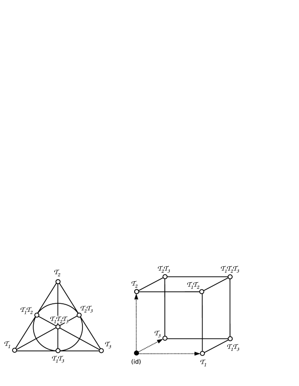
Figure 4.1. All unique automorphisms from repeat application of the $\left\{\mathcal{T}_{1},\mathcal{T}_{2},\mathcal{T}_{3}\right\}$ can be graphed in the Fano plane (left), where the product of each two automorphisms on a line yields the third. Together with identity $\left(\mathrm{id}\right)$ this forms the group $\mathbb{Z}_{2}^{3}=\mathbb{Z}_{2}\times\mathbb{Z}_{2}\times\mathbb{Z}_{2}$ (right).

Together with the identity element, $\left(\mathrm{id}\right)$, this forms the group $\mathbb{Z}_{2}^{3}=\mathbb{Z}_{2}\times\mathbb{Z}_{2}\times\mathbb{Z}_{2}$.

Together with the chirality-changing $\left\{\left(\mathrm{id}\right),\mathcal{T}_{0}\right\}\cong\mathbb{Z}_{2}$, the automorphism group between all the $f\left[N\right]$ is then:

$$\mathrm{Aut}\left(\left\{f_{\mathbb{O}}\left[N\right]\right\}\right) \cong\mathbb{Z}_{2}^{4}.$$

The $f\left[N\right]$ themselves are functions that map their of real arguments into the 7-sphere $S^{7}$, the unit sphere in $\mathbb{R}^{8}$:

$$f\left[N\right] : \mathbb{R}\otimes\ldots\otimes\mathbb{R}\rightarrow S^{7}.$$

Writing $\left[S^{7}\right]$ as the set of all functions on the 7-sphere, the symmetry $S^{D}$ of the generalized Born rule (4.3) becomes:

$$S^{D} \cong\left[S^{7}\right]\rtimes\mathbb{Z}_{2}^{4}.$$

Such $S^{D}$ is not a group due to nonassociativity of the $\left[S^{7}\right]$. It may instead have Hopf (co)quasigroup structure as in [23]. If true, it can be equipped with a differential calculus and Fourier transformation [24]. This mathematical flexibility would make it a promising structure to investigate the solution set of the generalized Born rule, which in turn would allow to identify applicability in physics.

4.3. Next steps and outlook

The prototype nonassociative quantum theory in one dimension was developed as a self-consistent formalism under the speculation that it may be further developed into a working quantum theory for the description of nature. Time and space will need to be modeled, and the set of solutions needs to be understood much deeper. Only then will it be possible to compare it with other models that are built from observed or speculated properties of nature.

Active and passive transformations here use exponentiation between an imaginary vector of unit length and a real number. These are the central pieces for modeling physical fields and particles. As a morphism over a two dimensional vector space, exponentiation $\mbox{\^{}}\,:\,\mathbb{R}^{2}\otimes\mathbb{R}^{2}\rightarrow\mathbb{R}^{2}$ in the complex numbers $\mathbb{C}$ is noncommutative, nonassociative, nonalternative, a left-inverse is generally different from a right inverse, and the morphism doesn’t distribute over addition. One might speculate about building new kinds of algebras from requiring existence of an exponential function that preserves a certain geometric simplicity, rather than attempting to preserve algebraic rules from pairwise morphisms (commutativity, associativity, distributivity, and similar). Two such examples in the two dimensional plane have been brought forward [38, 39], and may be of interest for evaluating new kinds of transformations for applicability in modeling nature.

In all, mathematical properties from nonassociative algebras, spinors, symmetries, and observed properties of nature at the smallest scales continue to offer enigmatic similarity, yet it is unclear whether nonassociativity in physics may ever overcome its current status of being an incidental curiosity: Are known circumstantial evidence and suspicious parallels the results of a yet undiscovered theory of consequence? Time (emergent or not) will tell.

Appendix A: Lorentz Lie algebra from nonassociative product

Section 2.2 shows the Lorentz Lie algebra,

(A.1) $$\left[M_{\mu\nu},M_{\rho\sigma}\right] =\imath\left(\eta_{\nu\rho}M_{\mu\sigma}+\eta_{\mu\sigma}M_{\nu\rho}-\eta_{\mu\rho}M_{\nu\sigma}-\eta_{\nu\sigma}M_{\mu\rho}\right),$$

$$\qquad\textrm{with }\mu,\nu,\rho,\sigma\in\left\{0,1,2,3\right\},$$

and states that this relation can be satisfied in the algebra of complex octonions $\mathbb{C}\otimes\mathbb{O}$ to basis $\left\{1,\imath\right\}\otimes\left\{1,i_{1},\ldots,i_{7}\right\}$ when defining [10, 27]:

$$R_{0} :=\frac{i_{4}}{2}\left(1+\imath\right), R_{j} :=\frac{i_{\left(j+4\right)}}{2}\left(1-\imath\right) \left(j\in\left\{1,2,3\right\}\right),$$

$$M_{\mu\nu} :=\frac{1}{2}\left[R_{\mu},R_{\nu}\right].$$

This appendix calculates relation (A.1) explicitly from the $R_{\mu}$ to provide proof:

Written in matrix form, the $M_{\mu\nu}$ are:

$$M_{\mu\nu}=\frac{1}{2}\left[R_{\mu},R_{\nu}\right] =\frac{1}{2}\left(\begin{array}[]{rrrr}0&i_{1}&i_{2}&i_{3}\\ -i_{1}&0&\imath i_{3}&\,-\imath i_{2}\\ -i_{2}&\,-\imath i_{3}&0&\imath i_{1}\\ -i_{3}&\imath i_{2}&-\imath i_{1}&0\end{array}\right).$$

The possible combinations of indices $\left\{\mu,\nu,\rho,\sigma\right\}$ from the Lorentz Lie algebra (A.1) fall in the following four cases:

• The case $M_{\mu\nu}=M_{\rho\sigma}$ is trivially satisfied.

• If $\mu=\nu$ or $\rho=\sigma$ then either $M_{\mu\nu}=0$ or $M_{\rho\sigma}=0$. The four terms of the right-hand side of relation (A.1) cancel each other out pairwise.

• If all four elements in $\left\{\mu,\nu,\rho,\sigma\right\}$ are different then $M_{\mu\nu}$ must be $\pm\imath M_{\rho\sigma}$:

  $$M_{01} =\frac{1}{2}\left[R_{0},R_{1}\right]=\frac{i_{1}}{2}=-\imath\frac{1}{2}\left[R_{2},R_{3}\right]=-\imath M_{23},$$

  $$M_{02} =\frac{1}{2}\left[R_{0},R_{2}\right]=\frac{i_{2}}{2}=\imath\frac{1}{2}\left[R_{1},R_{3}\right]=\imath M_{13},$$

  $$M_{03} =\frac{1}{2}\left[R_{0},R_{3}\right]=\frac{i_{3}}{2}=-\imath\frac{1}{2}\left[R_{1},R_{2}\right]=-\imath M_{12}.$$

  This makes the commutator $\left[M_{\mu\nu},M_{\rho\sigma}\right]=0$ as required per (A.1).

• The remaining case $\mu=\rho$ and $\nu\neq\sigma$ yields:

  $$\left[M_{01},M_{02}\right] =\frac{i_{3}}{2}=-\imath\eta_{00}M_{12}, \left[M_{01},M_{03}\right] =-\frac{i_{2}}{2}=-\imath\eta_{00}M_{13},$$

  $$\left[M_{12},M_{13}\right] =-\frac{i_{1}}{2}=-\imath\eta_{11}M_{23}, \left[M_{10},M_{13}\right] =\frac{\imath i_{3}}{2}=-\imath\eta_{11}M_{03},$$

  $$\left[M_{20},M_{21}\right] =\frac{\imath i_{1}}{2}=-\imath\eta_{22}M_{01}, \left[M_{20},M_{23}\right] =\frac{\imath i_{3}}{2}=-\imath\eta_{22}M_{03},$$

  $$\left[M_{30},M_{31}\right] =\frac{\imath i_{1}}{2}=-\imath\eta_{33}M_{01}, \left[M_{30},M_{32}\right] =\frac{\imath i_{2}}{2}=-\imath\eta_{33}M_{02}.$$

  All other index combinations are obtained from either switching the arguments of the commutator bracket, or from switching the indices of both $M$ terms. From the Minkowski tensor $\eta$ in (A.1) there will only be one nonzero term on the right-hand side. These are exactly the terms obtained from the complex octonion algebra of the $R_{\mu}$ above. $\square$

References

- [1] H. Albuquerque, S. Majid, “Quasialgebra structure of the octonions”, J. Algebra 220 (1999), 188-224; arXiv:math/9802116.
- [2] J. Baez, “The Octonions”, Bull. Amer. Math. Soc. 39 (2002), 145-205; arXiv:math/0105155.
- [3] J. C. Baez, J. Huerta, “Division Algebras and Supersymmetry I” in Superstrings, Geometry, Topology, and C*-algebras, eds. R. Doran, G. Friedman and J. Rosenberg; Proc. Symp. Pure Math. 81 (2010), 65-80; arXiv:0909.0551.
- [4] J. C. Baez, J. Huerta, “Division Algebras and Supersymmetry II” (2010); arXiv:1003.3436.
- [5] G. M. Dixon, “Division algebras: octonions, quaternions, complex numbers and the algebraic design of physics”, Springer (1994); also G. M. Dixon, “Division algebras; spinors; idempotents; the algebraic structure of reality” (2010); arXiv:1012.1304.
- [6] T. Dray, C. A. Manogue, “Quaternionic spin”, in Clifford Algebras and Their Applications in Mathematical Physics, eds. Rafał Abłamowicz and Bertfried Fauser; Birkhäuser (2000); arXiv:hep-th/9910010.
- [7] T. Dray, C. A. Manogue, “Octonionic Cayley Spinors and E6”, Comment. Math. Univ. Carolin. 51 (2010), 193–207; arXiv:0911.2255.
- [8] V. Dzhunushaliev, “Observables and unobservables in a non-associative quantum theory”, J. Gen. Lie Th. Appl. 2 (2008), 269-272; arXiv:quant-ph/0702263.
- [9] V. Dzhunushaliev, “Nonassociativity, supersymmetry, and hidden variables”, J. Math. Phys. 49 (2008), 042108; arXiv:0712.1647.
- [10] V. Dzhunushaliev, “Hidden structures in quantum mechanics”, J. Gen. Lie Th. Appl. 3 (2009), 33-38; arXiv:0805.3221.
- [11] V. Dzhunushaliev, “Hidden nonassociative structure in supersymmetric quantum mechanics”, Annalen Phys. 522 (2010), 382–388; arXiv:0904.2815.
- [12] V. Dzhunushaliev, “A nonassociative operator decomposition of strongly interacting quantum fields” (2009); arXiv:0906.1321.
- [13] V. Dzhunushaliev, “Nonperturbative quantum corrections” (2010); arXiv:1002.0180.
- [14] V. Dzhunushaliev, “SU(3) flux tube gluon condensate” (2010); arXiv:1010.1621.
- [15] C. Furey, “Unified theory of ideals” (2010); arXiv:1002.1497.
- [16] M. Gogberashvili, “Octonionic geometry”, Adv. Appl. Clifford Algebras 15 (2005), 55-66; arXiv:hep-th/0409173.
- [17] M. Gogberashvili, “Octonionic version of Dirac equations”, Int. J. Mod. Phys. A 21 (2006), 3513-3523; arXiv:hep-th/0505101.
- [18] M. Gogberashvili, “Octonionic electrodynamics”, J. Phys. A: Math. Gen. 39 (2006), 7099-7104; arXiv:hep-th/0512258.
- [19] M. Gogberashvili, “Rotations in the space of split octonions”, Adv. Math. Phys. 2009 (2009), 483079; arXiv:0808.2496.
- [20] M. Günaydin, F. Gürsey, “Quark structure and octonions”, J. Math. Phys. 14 (1973), 1651-1667.
- [21] M. Günaydin, F. Gürsey, “Quark statistics and octonions”, Phys. Rev. D. 9 (1974), 3387-3391.
- [22] M. Günaydin, C. Piron, H. Ruegg, "Moufang plane and octonionic Quantum Mechanics", Comm. Math. Phys. 61 (1978), 69-85.
- [23] J. Klim, S. Majid, “Hopf quasigroups and the algebraic 7-sphere” J. Algebra 323 (2010), 3067-3110; arXiv:0906.5026.
- [24] J. Klim, “Integral theory for Hopf (co)quasigroups” (2010); arXiv:1004.3929.
- [25] J. Köplinger, “Hypernumbers and relativity”, Appl. Math. Computation 188 (2007), 954-969.
- [26] J. Köplinger, “Gravity and electromagnetism on conic sedenions”, Appl. Math. Computation 188 (2007), 948-953.
- [27] J. Köplinger, “Nonassociative quantum theory on octooctonion algebra”, J. Phys. Math. 1 (2009), S090501.
- [28] J. Köplinger, “An analysis of Rick Lockyer’s ’octonion variance sieve”’ (2011); arXiv:1103.4748.
- [29] S. de Leo, K. Abdel-Khalek, "Octonionic quantum mechanics and complex geometry", Prog. Theor. Phys. 96 (1996), 823-831; arXiv:hep-th/9609032.
- [30] S. de Leo and K. Abdel-Khalek, "Octonionic Dirac equation", Prog. Theor. Phys. 96 (1996), 833-845; arXiv:hep-th/9609033.
- [31] S. de Leo and K. Abdel-Khalek, "Towards an octonionic world", Int. J. Theor. Phys. 37 (1998), 1945-1985; hep-th/9905123.
- [32] A. G. Lisi, “An exceptionally simple Theory of Everything” (2007); arXiv:0711.0770.
- [33] C. A. Manogue, T. Dray, “Dimensional reduction”, Mod. Phys. Lett. A14 (1999), 99-103; arXiv:hep-th/9807044.
- [34] C. A. Manogue, T. Dray, “Octonions, E6, and Particle Physics”, J. Phys.: Conf. Ser. 254 (2010), 012005; arXiv:0911.2253.
- [35] S. Okubo, “Introduction to octonion and other non-associative algebras in physics”, Cambridge University Press, Cambridge (1995).
- [36] R. D. Schafer, “An introduction to nonassociative algebras”, Dover Publications, New York (1995).
- [37] J. Schray, C. Manogue, “Octonionic representations of Clifford algebras and triality”, Foundations of Physics 26 (1996), 17-70; arXiv:hep-th/9407179.
- [38] J. A. Shuster, J. Köplinger, “Elliptic complex numbers with dual multiplication”, Appl. Math. Computation 216 (2010), 3497-3514.
- [39] J. A. Shuster, J. Köplinger, “Doubly nilpotent numbers in the 2D plane”, Appl. Math. Comput. 217 (2011), 7295-7310.