Classical 5D fields generated by a uniformly accelerated point source

Abstract

Gauge fields associated with the manifestly covariant dynamics of particles in $(3,1)$ spacetime are five-dimensional. In this paper we explore the old problem of fields generated by a source undergoing hyperbolic motion in this framework. The 5D fields are computed numerically using absolute time $\tau$-retarded Green-functions, and qualitatively compared with Maxwell fields generated by the same motion. We find that although the zero mode of all fields coincides with the corresponding Maxwell problem, the non-zero mode should affect, through the Lorentz force, the observed motion of test particles.

1 Introduction

The problem of Maxwell $(3,1)$ electromagnetic fields generated by a uniformly accelerated point source is an age old problem starting as early as 1909 by Max Born [7], followed by a plethora of papers and books.

The problem appears deceptively simple, and yet, it has raised many arguments and discussions on the very nature of radiation and inertial motion.

Locally, a uniformly accelerating source is essentially a notion from Newtonian Mechanics, mostly associated with a point mass in a static constant gravitational field, or an electric charge in similarly static and constant electric field. A covariant description of this motion corresponds to a hyperbola in a spacetime of $1+1$ dimensions, a worldline of the parametrized form

$$z(\tau) =z_{0}+\dfrac{1}{g}\cosh(g\tau)$$ (1)

$$t(\tau) =t_{0}+\dfrac{1}{g}\sinh(g\tau)$$ (2)

where $g$ is the Newtonian acceleration in the local frame (LF) $g=d^{2}z/dt^{2}|_{\text{LF}}$, and $\tau$ denotes proper time.

The main issues that have been debated are:

1. Uniform acceleration does not cause radiation reaction. It can be shown in the (mass renormalized) Lorentz-Dirac equation [10, 11, 8, 30]

   $$m\ddot{z}^{\mu} =\Gamma_{\text{ext}}^{\mu}+\Gamma_{\text{rr}}^{\mu}=\Gamma_{\text{ext}}^{\mu}+\dfrac{2e^{2}}{3c^{2}}\left[\dddot{z}^{\mu}+\dfrac{1}{c^{2}}\left(\ddot{z}^{\nu}\ddot{z}_{\nu}\right)\dot{z}^{\mu}\right]$$ (3)

   that the radiation reaction force term $\Gamma_{\text{rr}}^{\mu}$ vanishes for the motion described by (1) and (2). This apparent contradiction of the conservation of energy can be resolved [8, 28, 17, 39], either by limiting the time interval in which the particle is accelerated [14, 28, 27], or, alternatively, draining the apparent inexhaustible self-energy of the particle’s field [11]. Locally, uniform-acceleration has an event horizon at $x=t$, and cannot be influenced by events outside this cone. However, this means that locally, the charge is unaffected by its own loss of energy due to radiation.

   In the limit of unbounded accelerated motion, the balance of mechanical and electromagnetic energy becomes a balance of infinities, and is not well defined [39].

2. In the special inertial frame in which the source is momentarily at rest, the magnetic field vanishes for all space. This might lead to an apparent contradiction as the Poynting vector is zero everywhere in this frame, suggesting there is a lack of radiation, opposing the well known formula for overall radiation generated by an accelerating point source [34, 20]

   $$R =\dfrac{2e^{2}\ddot{z}_{\mu}\ddot{z}^{\mu}}{3c^{3}}$$

   This apparent contradiction is easily resolved (e.g. [11, 39]) by noting the fact that the magnetic field value ${\boldsymbol{H}}({\boldsymbol{x}},t_{0})$ on a given $t=t_{0}$ 3D surface depends on the entire history of the source particle (prior to $t_{0}$). However, the transfer of radiated energy follows along the light cone (via the conservation equation for the energy-momentum tensor $\theta^{\mu\nu}$), and not along space-like surfaces.

3. In the setting of general relativity, a somewhat more uncertain question remains: How does radiation transpire in the presence of a constant static background gravitational field? For instance, [8, 28, 39] claim that radiation takes place in the case of a fixed (supported) detector observing a point charge which undergoes geodesic (freefall) motion, whereas [36, 17] claim the opposite. The difference amongst claims has its roots in the very notion of radiation, of whether it is a property of space [17] or of the observer [28, 39].

In this paper, we examine the problem in a different framework, namely, the off-shell electrodynamics arising in the manifestly covariant relativistic dynamics of Stueckelberg [37, 38] and Horwitz and Piron [19, 35].

In this framework, a universal time $\tau$ is defined, parameterizing the motion of all events, which can be viewed schematically as $4D$ spacetime particles. Therefore, the resultant electromagnetic fields, which may depend on a spacetime point $x^{\mu}$ as well as $\tau$, generally obey a five dimensional linear wave-equation, in either $(4,1)$ or $(3,2)$ symmetry. Both the additional dimension and the requirement for causality in $\tau$, lead to a different support structure of the corresponding Green-function. The domain of dependence of a field $a^{\alpha}$ at a 5D observation point $(x^{\mu},\tau)$ is now the entire retarded $\tau$ history of the source inside the corresponding 5D past hyper-cone. Our conclusion is that there is indeed radiation in this configuration; even though the zero mode of the 5D fields coincides with the standard Maxwell fields, the Lorentz force due to the non-zero modes can have an effect on test particles.

Test particles moving according to this field may have worldlines substantially different from those predicted by the Maxwell theory. In the case of a source undergoing hyperbolic motion, the test particles can be shown to move highly above their mass shell.

Generally, a particle may follow any motion in spacetime, including spacelike motion, and reverse timelike motion, which would be interpreted by an observer as an anti-particle moving forward in time. The off-shell motion can be shown to result from transfer of mass to and from test particles by the field. The reverse temporal motion of a particle can be viewed according to Stueckelberg’s original view [37, 38] as a classical analog of the anti-particle.

Since the wave equation is in 5D, its support is the entire past $\tau$ history of the source. The Huygens’ principle does not apply, and thus, sources leave a trail, or a wake along their path.

Generally, the evaluation of the fields at any given 5D observation point $(x^{\mu},\tau)$ requires the entire history of the source inside the past cone with respect to this observation point. As this rarely yields closed-form analytic solutions, numerical computation is an essential tool in this investigation.

This work continues a previous study [1] on the fields generated by a point source in uniform motion.

The paper is organized as follows:

1. In section 2, we give a short overview of the manifestly covariant relativistic dynamics of Stueckelberg and the corresponding off-shell electrodynamics.

2. In 3 we provide the general $\tau$ retarded Green-Functions. These are derived from a ultrahyperbolic generalized Riemann-Liouville integro-differential operator, taken from Nozaki [26].

3. In 4 we discuss conditions in which the fields are regularizable.

4. In 5 we show the numerical results, and qualitatively compare the solution to the Maxwell case.

5. In the last section 6 we provide a summary and future prospects.

6. We also provide an appendix for a more detailed derivation of the $\tau$-retarded Green function, and the associated regularization.

2 Fundamentals

2.1 Stueckelberg mainfestly covariant relativistic dynamics

A so-called offshell classical and quantum electrodynamics has been constructed [35] from a fundamental theory of relativistic dynamics of 4D particles, termed events, in a framework first derived by Stueckelberg [37, 19].

Stueckelberg defined a Lorentz invariant Hamiltonian-like generator of evolution, over 8D phase space, with dynamics parameterized by a Lorentz invariant $\tau$, in both classical and quantum relativistic mechanics. Solutions of the relativistic quantum two body bound state problem, defined in terms of an invariant potential function, agree (up to relativistic corrections) with solutions of the non-relativistic Schrödinger equation [2, 4, 3]. The experiments of Lindner, et. al. [24], moreover, showing quantum interference in time can be explained in a simple and consistent way in the framework of this theory [18], and provides strong evidence that the time $t$, should be regarded as a quantum observable, as required in this framework.

In the classical manifestly covariant theory [37, 19], the Hamiltonian of a free particle is given by

$$K=\dfrac{p_{\mu}p^{\mu}}{2M}$$ (4)

where $x^{\mu}=[ct,{\boldsymbol{x}}]$ and $p^{\mu}=[E/c,{\boldsymbol{p}}]$. A simple model for an interacting system is provided by the potential model

$$K =\dfrac{p_{\mu}p^{\mu}}{2M}+V(x)$$ (5)

The Hamilton equations are (the dot indicates derivative with respect to the independent parameter $\tau$)

$$\dot{x}^{\mu}=\dfrac{\partial K}{\partial p_{\mu}}=\dfrac{1}{M}p^{\mu}\qquad\qquad\dot{p}^{\mu}=-\dfrac{\partial K}{\partial x_{\mu}}=-\dfrac{\partial V}{\partial x^{\mu}}$$ (6)

It follows from (6) that

$${\boldsymbol{v}} =\dfrac{d{\boldsymbol{x}}}{dt}=\dfrac{\dot{{\boldsymbol{x}}}}{\dot{t}}=\dfrac{{\boldsymbol{p}}}{E}$$

which is the standard formula obtained for velocity in special relativity (we take $c=1$ in the following).

Horwitz and Piron [19] generalized the framework to many-body systems, and gave $\tau$ the physical meaning of a universal historical time, correlating events in spacetime.

The general many-body, $\tau$ invariant, classical evolution function is defined as

$$K=\sum_{\scriptscriptstyle n=1}^{N}\dfrac{1}{2M_{n}}\eta_{\mu\nu}p_{n}^{\mu}p_{n}^{\nu}+V(x_{1},x_{2},...,x_{N})$$ (7)

where $\eta_{\mu\nu}=diag(-,+,+,+)$ and $n$ sums over all particles of the system, and, in this case, we have taken the potential function $V$ not to be a function of momenta or $\tau$. The classical equations of motion, for a single particle system in an external potential $V(x)$, are similar to the non-relativistic Hamilton equations,

$$\dot{x}_{n}^{\mu}=\dfrac{\partial K}{\partial p_{n\;\mu}}=\dfrac{1}{M_{n}}p_{n}^{\mu}\qquad\qquad\dot{p}_{n\;\mu}=-\dfrac{\partial K}{\partial x_{n}^{\mu}}=-\dfrac{\partial V}{\partial x_{n}^{\mu}}$$ (8)

In the usual formulation of relativistic dynamics (cf. [33]), the energy-momentum is constrained to a mass-shell defined as

$$p^{\mu}p_{\mu}=\mathbf{p}^{2}-E^{2}=-M^{2}$$ (9)

where $M$ is a given fixed quantity, a property of the particle. In the Stueckelberg formulation, however, the event mass is generally unconstrained. Since in (5), the value of $K$ is absolutely conserved, $p_{\mu}p^{\mu}=-m^{2}$ is constant only in the special case where

$$\dfrac{d}{d\tau}V(x)=\left[\dot{x}^{\mu}\dfrac{\partial}{\partial x^{\mu}}+\dfrac{\partial}{\partial\tau}\right]V(x)=\dot{x}\cdot\mathbf{\nabla}V(x)=0$$

In this case, the particle remains in a specific mass shell, which may or may not coincide with its so-called Galilean target mass, usually denoted by $M$. In the general case, however, $p^{\mu}p_{\mu}\equiv-m^{2}$ is a dynamical (Lorentz invariant) property, which may depend on $\tau$. The relation between $\tau$ and the proper time $s$, in the model of eq. (7), is given by

$$ds^{2} \equiv-dx^{\mu}dx_{\mu}=-\dot{x}^{\mu}\dot{x}_{\mu}d\tau^{2}=-\dfrac{1}{M^{2}}p^{\mu}p_{\mu}d\tau^{2}=\dfrac{m^{2}}{M^{2}}d\tau^{2}$$ (10)

Thus, the proper time $ds$, and universal time $d\tau$, are related through the ratio between the dynamical Lorentz invariant mass $m$, and the Galilean target mass $M$. If $V(x)$ goes to zero asymptotically, then it becomes constant. Since this asymptotic value is usually what is measured in experiment, we may assume that it takes on the value of the Galilean target mass. Although there are no detailed models at present, one assumes that there is a stabilizing mechanism (for example, self-interaction or, in terms of a minimal free energy in statistical mechanics as, for example, in condensation phenomena [9]) which brings the particle, at least to a good approximation, to a defined mass value, such that

$$K=\dfrac{1}{2M}p^{\mu}p_{\mu}=\dfrac{-m^{2}}{2M}=-\dfrac{M}{2}$$

For the quantum case, for which $p^{\mu}$ is represented by $-i\partial/\partial x_{\mu}$, the Stueckelberg Schrödinger equation is taken to be (we take $\hbar=1$ in the following)

$$i\dfrac{\partial\Psi_{\tau}(x)}{\partial\tau}=K\Psi_{\tau}(x)$$ (11)

The Stueckelberg classical and quantum relativistic dynamics have been studied for various systems in some detail, including the classical relativistic Kepler problem [19] and, as mentioned above, the quantum two body problem for a central potential [4].

2.2 Off-Shell Electrodynamics

What we shall call ”pre-Maxwell” off-shell electrodynamics is constructed in a similar fashion to the construction of standard Maxwell electrodynamics from the Schrödinger equation [35].

Under the local gauge transformation

$$\Psi^{\prime}_{\tau}(x)=e^{-ie_{0}\chi(x,\tau)}\Psi_{\tau}(x)$$ (12)

5 compensation fields $a^{\alpha}(x,\tau)$ ($\alpha\in\{0,1,2,3,5\}$) are implied, such that with the transformation

$$a^{\prime}_{\scriptscriptstyle\alpha}(x,\tau)=a_{\alpha}(x,\tau)-\partial_{\alpha}\chi(x,\tau)$$

the following modified Stueckelberg-Schrödinger equation remains form invariant

$$\left[i\dfrac{\partial}{\partial\tau}+e_{0}a_{5}(x,\tau)\right]\Psi_{\tau}(x)=\dfrac{1}{2M}\left[(p^{\mu}-e_{0}a^{\mu})(p_{\mu}-e_{0}a_{\mu})\right]\Psi_{\tau}(x)$$ (13)

under the transformation (12).

We can see this by observing the following relations:

$$\left[p_{\mu}-e_{0}a^{\prime}_{\mu}\right]\Psi^{\prime} =\left[-i\dfrac{\partial}{\partial x^{\mu}}-e_{0}\left(a_{\mu}-\dfrac{\partial}{\partial x^{\mu}}\chi\right)\right]e^{-ie_{0}\chi}\Psi=$$

$$=\left[-e_{0}\dfrac{\partial}{\partial x^{\mu}}\chi-i\dfrac{\partial\Psi}{x^{\mu}}-e_{0}\left(a_{\mu}-\dfrac{\partial\chi}{\partial x^{\mu}}\right)\right]e^{-ie_{0}\chi}\Psi=$$

$$=e^{-ie_{0}\chi}[p_{\mu}-e_{0}a_{\mu}]\Psi$$

and

$$\left[i\dfrac{\partial}{\partial\tau}+e_{0}(a_{5}-\dfrac{\partial\chi}{\partial\tau})\right]e^{-ie_{0}\chi}\Psi =\left[e_{0}\dfrac{\partial\chi}{\partial\tau}+i\dfrac{\partial\Psi}{\partial\tau}+e_{0}(a_{5}-\dfrac{\partial\chi}{\partial\tau})\right]e^{-ie_{0}\chi}\Psi=$$

$$=e^{-ie_{0}\chi}\left[i\dfrac{\partial}{\partial\tau}+e_{0}a_{5}\right]\Psi$$

The result is then, of the same form as for the usual $U(1)$ gauge compensation argument for the non-relativistic Schrödinger equation. Thus, the classical (and quantum) evolution function for a particle, under an external field, is then given by

$$K=\dfrac{1}{2M}\left[p-e_{0}a(x,\tau)\right]^{2}-e_{0}a^{5}(x,\tau)$$ (14)

(where we have used the shorthand notation of $x^{2}=x_{\mu}x^{\mu}$) and the corresponding Hamilton equations are

$$\dot{x}^{\mu}(\tau) =\dfrac{\partial K}{\partial p_{\mu}}=\dfrac{1}{M}\left[p^{\mu}-e_{0}a^{\mu}\right]$$ (15)

$$\dot{p}^{\mu}(\tau) =-\dfrac{\partial K}{\partial x_{\mu}}=\dfrac{e_{0}}{M}\left(p-e_{0}a(x,\tau)\right)_{\nu}\partial^{\mu}a^{\nu}(x,\tau)+e_{0}\partial^{\mu}a^{5}(x,\tau)$$ (16)

Here, $e_{0}$ is proportional to the Maxwell charge $e$ through a dimensional constant, which is discussed below. Second order equations of motion for $x^{\mu}(\tau)$, a generalization of the usual Lorentz force, follow from the Hamilton equations (15) and (16) [35]

$$M\ddot{x}^{\mu}=e_{0}\dot{x}^{\nu}f_{\;\nu}^{\mu}+e_{0}f_{\;5}^{\mu}$$ (17)

where for $\alpha,\beta=0,1,2,3,5$ the antisymmetric tensor

$$f^{\alpha\beta}\equiv\partial^{\alpha}a^{\beta}-\partial^{\beta}a^{\alpha}$$ (18)

is the (gauge invariant) 5D field tensor. Moreover, second order wave equation for the fields $f^{\alpha\beta}$ can be derived from a Lagrangian density as follows [35]:

$$\mathscr{L}=-\dfrac{\lambda}{4}f_{\alpha\beta}f^{\alpha\beta}-e_{0}a_{\alpha}j^{\alpha}$$ (19)

which produces the wave equation

$$\lambda\partial_{\alpha}f^{\beta\alpha}=e_{0}j^{\beta}$$ (20)

$\lambda$ is a dimensional constant, which will be shown below to have dimensions of length. The sources $j^{\beta}(x,\tau)$ depend both on spacetime and on $\tau$, and obey the continuity equation

$$\partial_{\alpha}j^{\alpha}=\partial_{\mu}j^{\mu}+\partial_{\tau}\rho=0$$ (21)

where $j^{5}\equiv\rho$ is a Lorentz invariant spacetime density of events. This equation follows from (13) for

$$\rho_{\tau}(x) =\Psi^{*}_{\tau}(x)\Psi_{\tau}(x)$$

$$j^{\mu}_{\tau}(x) =-\dfrac{i}{2M}\left[\Psi^{*}_{\tau}(x)\left(i\partial^{\mu}-e_{0}a^{\mu}(x,\tau)\right)\Psi_{\tau}(x)+c.c.\right]$$

as we discuss below, and also the classical from the argument given below.

2.2.1 Currents of point events

Jackson [20] showed that a conserved current for a moving point charge can be derived in a covariant way by defining the current as

$$J^{\mu}(x)=e\int_{-\infty}^{+\infty}\mathop{}\!\mathrm{d}s\,\dot{z}^{\mu}(s)\delta^{4}[x-z(s)]$$ (22)

In this case, $s$ is the proper time, and $z^{\mu}(s)$ the world-line of the point charge (for free motion, $s$ may coincide with $\tau$), and $\dot{z}^{\mu}(s)=\dfrac{d}{ds}z^{\mu}(s)$. Then,

$$\partial_{\mu}J^{\mu}=-e\int_{-\infty}^{+\infty}\mathop{}\!\mathrm{d}s\,\dfrac{\mathop{}\!\mathrm{d}}{\mathop{}\!\mathrm{d}s}\delta^{4}[x-z(s)]=-e\,\lim\limits_{L\rightarrow+\infty}\delta^{4}[x-z(s)]\Bigg{|}_{-L}^{+L}$$ (23)

which vanishes if $z^{\mu}(s)$ (or, for example, just the time component $z^{0}(s)$) becomes infinite for $s\rightarrow\pm\infty$, and the observation point $x^{\mu}$ is restricted to a bounded region of spacetime, e.g., the laboratory. We therefore, with Jackson, identify $J^{\mu}$ as the Maxwell current. We see that this current is a functional on the world line, and the usual notion of a ”particle” associated with a conserved 4-current (and therefore a charge charge corresponding to the space integral of the fourth component), corresponds to this functional on the world line.

If we identify $\delta^{4}[x-z(s)]$ with a density $\rho_{s}(x)$ and the local (in $\tau$) current $\dot{z}^{\mu}(s)\delta^{4}[x-z(s)]$ with a local current $j^{\mu}_{s}(x)$

$$\rho_{s}(x)=\delta^{4}[x-z(s)]\qquad\qquad j^{\mu}(x,s)=\dot{z}^{\mu}(s)\delta^{4}[x-z(s)]$$ (24)

then the relation

$$\dfrac{d}{ds}\delta^{4}[x-z(s)]=-\dot{z}^{\mu}(s)\partial_{\mu}\delta^{4}[x-z(s)]$$

used in the above demonstration in fact corresponds to the conservation law (reverting to the more general parameter $\tau$ in place of the proper time $s$) (21)

$$\partial_{\mu}j^{\mu}(x,\tau)+\partial_{\tau}\rho(x,\tau)=0$$ (25)

What we call the pre-Maxwell current of a point event is then defined as

$$j^{\alpha}(x,\tau)=\dot{z}^{\alpha}(\tau)\delta^{4}[x-z(\tau)]$$ (26)

where $j^{5}(x,\tau)\equiv\rho(x,\tau)$ and $\dot{z}^{5}(\tau)\equiv 1$ (since $z^{5}(\tau)\equiv\tau$). Integrating (20) over $\tau$, we recover the standard Maxwell equations for Maxwell fields defined by

$$A^{\mu}(x) =\int a^{\mu}(x,\tau)\mathop{}\!\mathrm{d}\tau$$ (27)

We therefore call the fields $a^{\mu}(x,\tau)$ pre-Maxwell fields. From (19)

$$\lambda\int_{-\infty}^{+\infty}\left[\partial_{\mu}f^{\mu\nu}(x,\tau)+\partial_{5}f^{\mu 5}(x,\tau)\right]\mathop{}\!\mathrm{d}\tau =\lambda\int_{-\infty}^{+\infty}\partial_{\alpha}f^{\mu\alpha}(x,\tau)\mathop{}\!\mathrm{d}\tau$$

$$=e_{0}\int_{-\infty}^{+\infty}j_{\beta}(x,\tau)\,\mathop{}\!\mathrm{d}\tau$$

$$=e_{0}\dfrac{1}{e}J^{\mu}(x)$$ (28)

where the $\tau$ integral of $\partial_{5}f^{\mu 5}$ vanishes for local sources. Therefore, (28) proves (27). Moreover,

$$\partial_{\nu}F^{\mu\nu} =\dfrac{e_{0}}{\lambda e}J^{\mu}(x)$$ (29)

we find the constants $\lambda$ and $e_{0}$ are related by

$$\lambda =\dfrac{e_{0}}{e}$$ (30)

$$e =\dfrac{e_{0}}{\lambda}$$ (31)

where $e$ is the standard Maxwell charge.

For the quantum theory, a real positive definite density function $\rho_{\tau}(x)$ can be derived from the Stueckelberg-Schrödinger equation (11)

$$\rho_{\tau}(x)=|\Psi_{\tau}|^{2}=\Psi^{*}_{\tau}(x)\Psi_{\tau}(x)$$ (32)

which can be identified with the $\rho(x,\tau)=\delta^{4}[x-z(\tau)]$ in the classical (relativistic) limit. It follows from the Stueckelberg equation (13) that the continuity equation (25) is then satisfied for the gauge invariant current

$$j^{\mu}_{\tau}(x)=-\dfrac{1}{2M}\left[\Psi^{\ast}_{\tau}(x)(i\partial^{\mu}-e_{0}a^{\mu}(x,\tau))\Psi_{\tau}(x)+\text{c.c.}\right]$$ (33)

From (19), also valid for the quantum theory [35, 23], and (27), we find

$$J^{\mu}(x)=e\int_{-\infty}^{+\infty}j^{\mu}(x,\tau)\,\mathop{}\!\mathrm{d}\tau$$ (34)

2.2.2 The wave equation

From equations (20) and (18) one can derive the wave equation for the potentials $a^{\scriptscriptstyle\alpha}(x,\tau)$:

$$\lambda\partial_{\beta}\partial^{\beta}a^{\alpha}-\lambda\partial^{\alpha}(\partial_{\beta}a^{\beta})=e_{0}\,j^{\alpha}$$ (35)

Under the generalized Lorentz gauge $\partial_{\beta}a^{\scriptscriptstyle\beta}=0$, the wave equation takes the simpler form

$$\lambda\partial_{\beta}\partial^{\beta}a^{\alpha}=\lambda\left[\Box^{2}a^{\alpha}+\sigma_{5}\dfrac{\partial^{2}a^{\alpha}}{\partial\tau^{2}}\right]=e_{0}\,j^{\alpha}(x,\tau)$$ (36)

where a $5^{th}$ diagonal metric component can take either signs $\sigma_{5}=\pm 1$, corresponding to $O(4,1)$ and $O(3,2)$ symmetries of the homogeneous field equations, respectively.

Integrating (36) with respect to $\tau$, and assuming that $\lim\limits_{\tau\rightarrow\pm\infty}\partial_{\tau}a^{\alpha}(x,\tau)=0$, we obtain

$$\lambda\int_{-\infty}^{+\infty}\mathop{}\!\mathrm{d}\tau\,\left[\Box^{2}a^{\alpha}+\sigma_{5}\dfrac{\partial^{2}a^{\alpha}}{\partial\tau^{2}}\right]=\dfrac{e_{0}}{e}J^{\alpha}(x)$$

Identifying

$$A^{\mu}(x)=\int_{-\infty}^{+\infty}\mathop{}\!\mathrm{d}\tau\,a^{\mu}(x,\tau)$$ (37)

we obtain

$$\lambda\Box^{2}A^{\mu}(x) =\dfrac{e_{0}}{e}J^{\mu}(x)$$

i.e.

$$\Box^{2}A^{\mu}(x) =J^{\mu}(x)$$

(for $\mu=0,1,2,3$)

Therefore, the Maxwell electrodynamics is properly contained in the 5D electromagnetism.

2.2.3 A note about units

In natural units ($\hbar=c=1$), the Maxwell potentials $A^{\mu}$ have units of $1/L$. Therefore, the pre-Maxwell OSE potentials $a^{\alpha}$ have units of $1/L^{2}$, and in order to maintain the action integral

$$S=\int_{-\infty}^{+\infty}\mathscr{L}\,\mathop{}\!\mathrm{d}\tau\,\mathop{}\!\mathrm{d}^{4}x$$ (38)

dimensionless, the coefficient $\lambda$ in (19) must have units of $L$, forcing $e_{0}$ to have units of $L$ as well (hence $e$ is dimensionless).

The Fourier transform of the pre-Maxwell OSE fields

$$\tilde{a}^{\mu}(x,s)=\int_{-\infty}^{+\infty}e^{is\tau}a^{\mu}(x,\tau)\,\mathop{}\!\mathrm{d}\tau$$ (39)

and equation (37) suggest that the Maxwell potentials and fields correspond to the zero mode of the pre-maxwell OSE fields, with respect to $\tau$, i.e.,

$$A^{\mu}(x)=\tilde{a}^{\mu}(x,s)|_{s=0}$$ (40)

2.3 Solutions of the wave equation

In [1], we have shown the Green-functions (GF) associated with the 5D wave-equation (36) that are consistent with uniformly moving point sources are

$$g_{\sigma_{5}}(x,\tau)=\dfrac{\sigma_{5}}{4\pi^{2}}\lim\limits_{\epsilon\to 0^{+}}\dfrac{\partial}{\partial\epsilon}\dfrac{\theta[-\sigma_{5}\left(x^{2}+\sigma_{5}\tau^{2}\right)+\epsilon]}{\sqrt{-\sigma_{5}\left(x^{2}+\sigma_{5}\tau^{2}\right)+\epsilon}}$$ (41)

where $\sigma_{5}=\pm 1$ for the sign of $\tau$ in the metric, $\pm 1$ for $(4,1)$ and $(3,2)$ respectively, obeying the wave equation on for a $\delta^{5}(x,\tau)$ source

$$\partial_{\beta}\partial^{\beta}a^{\alpha}(x,\tau) =\delta^{4}(x)\delta(\tau)$$ (42)

Using the GF’s (41) the general field generated by a given source can then be found by integration on its support

$$a^{\alpha}(x,\tau)=e_{0}\int\mathop{}\!\mathrm{d}^{4}x^{\prime}\,\mathop{}\!\mathrm{d}\tau^{\prime}\,g(x-x^{\prime},\tau-\tau^{\prime})\,j^{\alpha}(x^{\prime},\tau^{\prime})$$ (43)

and applying it to a point particle given by (24). The potentials of point events are then given as

$$a^{\alpha}(x,\tau)=e_{0}\int_{-\infty}^{+\infty}\mathop{}\!\mathrm{d}\tau^{\prime}\,g(x-z(\tau^{\prime}),\tau-\tau^{\prime})\,\dot{z}^{\alpha}(\tau^{\prime})$$ (44)

However, in the framework of off-shell electrodynamics, the fields are to be causal in $\tau$, and since (41) is symmetric with respect to $\tau$, they cannot be used for non-inertial (hence, non-uniform) source motion, as the notion of flow of radiation in $\tau$ is not properly accounted for (cf. [30]). Therefore, the next section is focused on achieving consistent $\tau$-retarded GF’s.

3 Retarded Green Functions

3.1 Retarded ultrahyperbolic Green-Functions

The generalization of potential theory to a spacetime with $(p,q)$ signature was achieved by Nozaki [26], that extended earlier work of Riesz [31, 32], on its own a generalization of potential theory to the Lorentzian space $(p,1)$.

It begins with a definition of a ultrahyperbolic distance between two points $x,y\in\mathbb{R}^{p,q}$

$$r^{2}(x-y) \equiv\eta_{ij}^{(p,q)}(x^{i}-y^{i})(x^{j}-y^{j})$$ (45)

where $\eta^{(p,q)}_{ij}$ is the corresponding $\mathbb{R}^{p,q}$ metric

$$\eta^{(p,q)}_{ij} =\text{diag}(\overbrace{+1,\ldots,+1}^{p},\overbrace{-1,\ldots,-1}^{q})$$ (46)

Then, the ultrahyperbolic inverted hypercone $\mathcal{D}_{x}$ with a vertex at $x\in\mathbb{R}^{p,q}$ is given by

$$\mathcal{D}_{x} =\left\{\xi\in\mathbb{R}^{p,q}\Big{|}\quad r^{2}(x-\xi)=\eta^{(p,q)}_{ij}(x^{i}-\xi^{i})(x^{j}-\xi^{j})>0,\quad x_{1}-\xi_{1}>0\right\}$$ (47)

$\mathcal{D}_{x}$ is in fact, the retarded hyper-cone, with respect to the first coordinate $x_{1}$.

A generalized Riemann-Liouville integration operator $J^{\alpha}$ is then defined by

$$J^{\alpha}f(x) =\int_{\mathcal{D}_{x}}\dfrac{r^{\alpha-m}(y)}{K_{m}(\alpha)}f(x-y)\,\mathop{}\!\mathrm{d}y=\Phi_{\alpha}(y)*f(x-y)$$ (48)

where $m=p+q$ is the dimensionality of the entire ultrahyperbolic space, and

$$r^{a}(x) =\left[r^{2}(x)\right]^{a/2}$$ (49)

and $*$ denotes convolution, where

$$\Phi_{\alpha}(y) \equiv\dfrac{r^{\alpha-m}(y)}{K_{m}(\alpha)}$$ (50)

$K_{m}(\alpha)$ is a normalization constant that is determined by fixing $J^{\alpha}$ such that the function $f(x)=e^{x_{1}}$ remains stationary under the action of $J^{\alpha}$.

Furthermore,

$$K_{m}(\alpha) =\pi^{(m-1)/2}\dfrac{\Gamma\left(\frac{\alpha-m+2}{2}\right)\Gamma\left(\alpha\right)\Gamma\left(\frac{1-\alpha}{2}\right)}{\Gamma\left(\frac{\alpha-p+2}{2}\right)\Gamma\left(\frac{p-\alpha}{2}\right)}$$ (51)

$K_{m}(\alpha)$ can be thought as a ultrahyperbolic generalization of the $\Gamma$-function. Using its analytic properties, it can be shown that [26]

$$\lim\limits_{\alpha\to 0^{+}}J^{\alpha}f(x) =f(x)$$

and thus

$$\lim\limits_{\alpha\to 0^{+}}\Phi_{\alpha}(x) =\delta(x)$$ (52)

Furthermore, the ultrahyperbolic wave-operator given by

$$\Delta \equiv\eta^{ij}_{(p,q)}\partial_{i}\partial_{j}$$ (53)

can be shown to obey

$$\Delta J^{\alpha}f(x) =J^{\alpha-2}f(x)$$

Or

$$\Delta\Phi_{\alpha}(x) =\Phi_{\alpha-2}(x)$$ (54)

Using (54) and (52), it can easily be seen that the fundamental-solution for the wave operator is

$$\Delta\lim\limits_{\alpha\to 0^{+}}\Phi_{\alpha+2}(x) =\Phi_{0}(x)$$

Thus

$$g_{(p,q)}(x) =\Phi_{2}(x)=\dfrac{r_{+}^{2-m}(x)}{K_{m}(2)}$$ (55)

3.2 Modified retarded ultrahyperbolic Green-Functions

Equation (41) is based a simple Principal Part solution based on Fourier analysis [1] of (42), and carries a negative signature for $\tau^{2}$ term in both $(4,1)$ and $(3,2)$ metrics. We therefore seek a general retarded ultrahyperbolic fundamental solution on a hyper-cone for which retardation vertex is determined by $x_{m}$. In the appendix B, we apply a procedure similar to Nozaki’s to obtain the required opposite signature retardation (this result may also be obtained by analytic continuation of B).

Beginning with the definition of the retarded inverted hypercone in $(p,q)$ with vertex at $x\in R^{p,q}$ by:

$$\mathcal{D^{\prime}}_{x} =\left\{\xi\in\mathbb{R}^{p,q}\Big{|}\quad r^{2}(x-\xi)=\eta^{(p,q)}_{ij}(x^{i}-\xi^{i})(x^{j}-\xi^{j})>0,\quad x_{m}-\xi_{m}>0\right\}$$ (56)

We similarly define a modified ultrahyperbolic Riemann-Liouville operator $L^{\alpha}$ such that

$$L^{\alpha}f(x) =(f*\phi_{\alpha})(x)=\int_{\mathcal{D^{\prime}}_{x}}\dfrac{r_{+}^{\alpha-m}(x-y)}{N_{m}(\alpha)}f(y)\,\mathop{}\!\mathrm{d}y$$ (57)

where, similarly to Nozaki’s construction of $K_{m}(\alpha)$,

$$N_{m}(\alpha) =2\pi^{(m-3)/2}\sin\left(\dfrac{\pi p}{2}\right)\Gamma\left(\dfrac{2+\alpha-m}{2}\right)\Gamma\left(\dfrac{1-\alpha}{2}\right)\Gamma\left(\alpha\right)$$ (58)

where in this case

$$\Delta\Phi_{\alpha}(x) =\Delta\dfrac{r_{+}^{\alpha-m}}{N_{m}(\alpha)}=-\Phi_{\alpha-2}(x)$$

and thus, the desired retarded GF’s are ($x\in\mathbb{R}^{p,q}$):

$$g_{(p,q)}(x) =-\lim_{\alpha\to 2}\Phi_{\alpha}(x)=\dfrac{r_{+}^{2-m}}{2\pi^{m/2-1}\sin\left(\dfrac{\pi p}{2}\right)\Gamma\left(\dfrac{4-m}{2}\right)}$$ (59)

Applying (59) to the case of $(4,1)$ or $(3,2)$ metrics, we find:

$$g(x) =\dfrac{\theta(\tau)}{4\pi^{2}}\begin{cases}(-1)\dfrac{\theta(-x^{2}-\tau^{2})}{(-x^{2}-\tau^{2})^{3/2}}\qquad\qquad&(4,1)\\ \dfrac{\theta(x^{2}-\tau^{2})}{(x^{2}-\tau^{2})^{3/2}}&(3,2)\end{cases}$$ (60)

which complies with the GF’s obtained in [1], aside from a factor of $2$, due to the specific choice of retarded GF. This is in exact analogy to the Maxwell GF’s in which

$$G_{\text{P}}(x) =\dfrac{1}{2}\left[G_{\text{ret}}(x)+G_{\text{adv}}(x)\right]$$

Following the convention [22, 1], we denote the sign of $\tau$ in the metric by $\sigma_{5}$, and define $R(x)=-\sigma_{5}(x^{2}+\sigma_{5}\tau^{2})$, we then find

$$g(x) =-\sigma_{5}\dfrac{\theta(\tau)}{4\pi^{2}}\dfrac{\theta(R(x))}{R^{3/2}(x)}$$

When a source $j^{\alpha}(x)$ is given, we find the field

$$a^{\alpha}(x) =\int_{\mathcal{D}_{x,x^{\prime}}}g(x-x^{\prime})j^{\alpha}(x^{\prime})\mathop{}\!\mathrm{d}x^{\prime}=-\dfrac{\sigma_{5}}{4\pi^{2}}\int_{\mathbb{R}^{5}}\theta(\tau-\tau^{\prime})\dfrac{\theta(R(x-x^{\prime}))}{R^{3/2}(x-x^{\prime})}\,j^{\alpha}(x^{\prime})\,dx^{\prime}$$ (61)

The integration over regions where $R(x-x^{\prime})=0$ is defined in the sense of generalized-functions, as given in [13], by employing canonical regularization (see appendix A).

For a point particle, $j^{\alpha}$ is

$$j^{\alpha}(x,\tau) =q\dfrac{dz^{\alpha}}{d\tau}\delta^{4}\left(x-z(\tau)\right)$$ (62)

where $z^{\alpha}(\tau)$ is the spacetime position of the source charge, and by definition, $z^{5}(\tau)\equiv\tau$. Inserting (62) to (61), we find

$$a^{\alpha}(x)=-\dfrac{q\sigma_{5}}{4\pi^{2}}\mathcal{R}\int_{-\infty}^{\tau}\dfrac{\theta\left(R(x-z(\tau^{\prime}))\right)}{R^{3/2}(x-z(\tau^{\prime}))}\,\dot{z}^{\alpha}(\tau^{\prime})\,\mathop{}\!\mathrm{d}\tau^{\prime}$$ (63)

where we explicitly denoted regularization by $\mathcal{R}$.

Similarly, the fields can be found by taking the spacetime-$\tau$ derivatives

$$f^{\alpha\beta}(x) =\partial^{\alpha}a^{\beta}-\partial^{\beta}a^{\alpha}=\dfrac{3q\sigma_{5}}{8\pi^{2}}\mathcal{R}\int_{-\infty}^{\tau}\dfrac{\theta\left(R\right)}{R^{5/2}}\,\left[\dot{z}^{\beta}\partial^{\alpha}R-\dot{z}^{\alpha}\partial^{\beta}R\right]\,\mathop{}\!\mathrm{d}\tau^{\prime}$$ (64)

where $R$ and $z^{\alpha}$ are evaluated at $\tau^{\prime}$. Hence forward, we shall denote by $R(\tau^{\prime})$ the expression

$$R(\tau^{\prime}) =-\sigma_{5}(x_{\alpha}-z_{\alpha}(\tau^{\prime}))(x^{\alpha}-z^{\alpha}(\tau^{\prime}))=-\sigma_{5}\left[(x-z(\tau^{\prime}))^{2}+\sigma_{5}(\tau-\tau^{\prime})^{2}\right]$$ (65)

3.3 Regularization

Integrals (64) and (63) are divergent at $\tau^{\prime}=\tau^{\prime}_{i}$, where $\tau^{\prime}_{i}$ are the roots of the equation $R(\tau^{\prime}_{i})=0$ with the additional constraint of retardation $\tau^{\prime}_{i}\leq\tau$. The divergence can be eliminated by following a procedure of canonical regularization [13] (see also appendix A). For example, let us assume that for a particular 5D observation $(x,\tau)$, the equation $R(\tau^{\prime})=0$ has a single root $\tau^{\prime}_{0}$ such that $R(\tau^{\prime}_{0})=0$, and $R(\tau^{\prime})<0$ for $\tau^{\prime}<\tau^{\prime}_{0}$.

Regularization of (64) can then be expressed as a sum of 3 operators, which are parameterized by a (small) $h$, as follows:

$$\mathcal{R} \int_{\tau^{\prime}_{0}}^{\tau}\dfrac{\phi^{\alpha\beta}(\tau^{\prime})}{R^{5/2}(\tau^{\prime})}\,\mathop{}\!\mathrm{d}\tau^{\prime}=\left[\mathcal{R}_{1}[h]+\mathcal{R}_{2}[h]+\mathcal{R}_{3}[h]\right]\int_{\tau^{\prime}_{0}}^{\tau}\dfrac{\phi^{\alpha\beta}(\tau^{\prime})}{R^{5/2}(\tau^{\prime})}\,\mathop{}\!\mathrm{d}\tau^{\prime}$$

$$=\int_{\tau^{\prime}_{0}}^{\tau^{\prime}_{h}}\dfrac{\dot{R}(\tau^{\prime})}{R^{5/2}(\tau^{\prime})}\left[\dfrac{\phi^{\alpha\beta}(\tau^{\prime})}{\dot{R}(\tau^{\prime})}-\dfrac{\phi^{\alpha\beta}(\tau^{\prime}_{0})}{\dot{R}(\tau^{\prime}_{0})}-R(\tau^{\prime})\left(\dfrac{\dot{\phi}^{\alpha\beta}(\tau^{\prime}_{0})}{\dot{R}^{2}(\tau^{\prime}_{0})}-\dfrac{\phi^{\alpha\beta}(\tau^{\prime}_{0})\ddot{R}(\tau^{\prime}_{0})}{\dot{R}^{3}(\tau^{\prime}_{0})}\right)\right]\mathop{}\!\mathrm{d}\tau^{\prime}+$$

$$\qquad+\left[\dfrac{\phi^{\alpha\beta}(\tau^{\prime}_{0})}{\dot{R}(\tau^{\prime}_{0})R_{h}^{3/2}}\left(1-3\dfrac{R_{h}\ddot{R}(\tau^{\prime}_{0})}{\dot{R}^{2}(\tau^{\prime}_{0})}\right)+3\dfrac{\dot{\phi}^{\alpha\beta}(\tau^{\prime}_{0})}{\dot{R}^{2}(\tau^{\prime}_{0})R_{h}^{1/2}}\right]+$$

$$\qquad+\int_{\tau^{\prime}_{h}}^{\tau}\dfrac{\phi^{\alpha\beta}(\tau^{\prime})}{R^{5/2}(\tau^{\prime})}\,\mathop{}\!\mathrm{d}\tau^{\prime}$$ (66)

where

$$\phi^{\alpha\beta}(\tau^{\prime}) \equiv\dot{z}^{\beta}(\tau^{\prime})\partial^{\alpha}R(\tau^{\prime})-\dot{z}^{\alpha}(\tau^{\prime})\partial^{\beta}R(\tau^{\prime})$$

$$\tau^{\prime}_{h} =\tau^{\prime}_{0}+h>\tau^{\prime}_{0}$$

$$R_{h} =R(\tau^{\prime}_{0}+h)$$

$$\dot{R}(\tau^{\prime}) =\dfrac{d}{d\tau^{\prime}}R(\tau^{\prime})$$

$$\mathcal{R}_{1}[h] \int_{\tau^{\prime}_{0}}^{\tau}\dfrac{\phi^{\alpha\beta}(\tau^{\prime})}{R^{5/2}(\tau^{\prime})}\,\mathop{}\!\mathrm{d}\tau^{\prime}=\int_{\tau^{\prime}_{0}}^{\tau^{\prime}_{h}}\dfrac{\dot{R}(\tau^{\prime})}{R^{5/2}(\tau^{\prime})}\left[\dfrac{\phi^{\alpha\beta}(\tau^{\prime})}{\dot{R}(\tau^{\prime})}-\dfrac{\phi^{\alpha\beta}(\tau^{\prime}_{0})}{\dot{R}(\tau^{\prime}_{0})}-R(\tau^{\prime})\left(\dfrac{\dot{\phi}^{\alpha\beta}(\tau^{\prime}_{0})}{\dot{R}^{2}(\tau^{\prime}_{0})}-\dfrac{\phi^{\alpha\beta}(\tau^{\prime}_{0})\ddot{R}(\tau^{\prime}_{0})}{\dot{R}^{3}(\tau^{\prime}_{0})}\right)\right]\mathop{}\!\mathrm{d}\tau^{\prime}$$

$$\mathcal{R}_{2}[h] \int_{\tau^{\prime}_{0}}^{\tau}\dfrac{\phi^{\alpha\beta}(\tau^{\prime})}{R^{5/2}(\tau^{\prime})}\,\mathop{}\!\mathrm{d}\tau^{\prime}=\dfrac{\phi^{\alpha\beta}(\tau^{\prime}_{0})}{\dot{R}(\tau^{\prime}_{0})R_{h}^{3/2}}\left(1-3\dfrac{R_{h}\ddot{R}(\tau^{\prime}_{0})}{\dot{R}^{2}(\tau^{\prime}_{0})}\right)+3\dfrac{\dot{\phi}^{\alpha\beta}(\tau^{\prime}_{0})}{\dot{R}^{2}(\tau^{\prime}_{0})R_{h}^{1/2}}$$

$$\mathcal{R}_{3}[h] \int_{\tau^{\prime}_{0}}^{\tau}\dfrac{\phi^{\alpha\beta}(\tau^{\prime})}{R^{5/2}(\tau^{\prime})}\,\mathop{}\!\mathrm{d}\tau^{\prime}=\int_{\tau^{\prime}_{h}}^{\tau}\dfrac{\phi^{\alpha\beta}(\tau^{\prime})}{R^{5/2}(\tau^{\prime})}\,\mathop{}\!\mathrm{d}\tau^{\prime}$$

The 3 operators $\mathcal{R}_{i}[h],i=1,2,3$ can be understood as follows:

1. $\mathcal{R}_{1}[h]$ regularizes the integral at the singularity point, by removing a sufficient number of terms from the numerator (2 terms for the power of $5/2$). The integration is over a small segment $(\tau^{\prime}_{0},\tau^{\prime}_{h})$.

2. $\mathcal{R}_{2}[h]$ adds the removed terms at the upper boundary $\tau^{\prime}_{h}=\tau^{\prime}_{0}+h$.

3. $\mathcal{R}_{3}[h]$ adds the remainder of the integral, which by assumption, is well-defined, since $R(\tau^{\prime})$ has no more roots in the remaining interval $(\tau^{\prime}_{h},\tau)$.

The parameter $h$ should satisfy the following constraints:

1. $\dot{R}(\tau^{\prime})\neq 0$ for $\tau^{\prime}_{0}<\tau^{\prime}<\tau^{\prime}_{h}$. This ensures that $\mathcal{R}_{1}[h]$ and $\mathcal{R}_{2}[h]$ are well-defined.

2. $h$ cannot be vanishingly small, since that would make the terms contributed by $\mathcal{R}_{2}[h]$ and $\mathcal{R}_{3}[h]$ divergent.

There are cases, depending on the observation point $(x,\tau)$, where the above constraints cannot be met, being either mutually exclusive or unattainable altogether (these cases correspond to similar conditions in which Maxwell fields would be divergent as well.).

The regularization scheme outlined above, based on the theory of regularization of generalized functions given in Gel’fand [13], is used quite frequently in numerical integration of hypersingular integrals (cf. [40] and references therein). Indeed, we have used (3.3) in the numerical evaluation of $f^{\alpha\beta}$. Similar methods are mentioned in other classical higher dimension electrodynamics applications [12, 21, 16] and and in many examples in quantum field theory.

4 Conditions for regularizability

4.1 Behavior at singularities

As $R(\tau^{\prime})$ can be understood as a Lorentzian squared distance between the observation point $(x,\tau)$ and the source point $(x(\tau^{\prime}),\tau^{\prime})$, the derivative $\dot{R}(\tau^{\prime})$ which can be written as

$$\dot{R}(\tau^{\prime}) =2\dot{z}^{\alpha}(\tau^{\prime})(x^{\alpha}-z^{\alpha}(\tau^{\prime}))$$ (67)

is normally interpreted as the spatial distance between the observation point and source point in the frame where the source is momentarily at rest. However, as events associated with timelike particles are not at rest in the temporal sense nor in the $\tau$ sense, there is no physical frame in which $\dot{R}(\tau^{\prime})$ is a pure spatial distance.

In the case of $(3,1)$ Maxwell electrodynamics, $\dot{R}(\tau^{\prime})$ is the denominator of the Liénard-Wiechert potentials, which has the well known form

$$A^{\mu}(x) =\dfrac{e\dot{z}^{\mu}(s_{0})}{4\pi\dot{z}_{\mu}(s_{0})(x^{\mu}-z^{\mu}(s_{0}))}=\dfrac{e\dot{z}^{\mu}(s_{0})}{2\pi\dot{R}(s_{0})}$$ (68)

where $s_{0}$ is defined as the retardation point

$$R(s_{0}) =0=-(x_{\mu}-z_{\mu}(s_{0}))(x^{\mu}-z^{\mu}(s_{0}))$$

with the extra retardation condition $t>z^{0}(s_{0})$.

The case of $\dot{R}(\tau^{\prime})=0$ is indeed interpreted as where the fields are normally singular, unless higher order regularization is employed, since they amount to observing the field on the particle itself. Therefore, in our case as well as in Maxwell electrodynamics, the case of $R(s_{0})=\dot{R}(s_{0})=0$ leads to $|A^{\mu}(x)|\to\infty$.

As $R(\tau^{\prime})$ reflects the squared timelike Lorentzian distance, the Green-function support peaks on the light cone $R(\tau^{\prime}_{0})=0$ for both even and odd spacetime dimensions. Therefore, the combined condition

$$R(\tau^{\prime}_{0})=\dot{R}(\tau^{\prime}_{0})=0$$

indicates that to first order, the wavefront remains on the same observation point, forming a discontinuity in the value of the field, similar to a shockwave front.

4.2 Dependence on source motion

By defining explicitly the distance 5-vector $\sigma^{\alpha}(\tau^{\prime})\equiv x^{\alpha}-z^{\alpha}(\tau^{\prime})$, and using some elementary spacetime vector algebra, the following can be shown straightforward:

• For a common root $\tau^{\prime}_{0}$ such that $R(\tau^{\prime})=\dot{R}(\tau^{\prime}_{0})=0$, we have:

  • $\sigma^{\alpha}(\tau^{\prime}_{0})\sigma_{\alpha}(\tau^{\prime}_{0})=0$ by definition of $R(\tau^{\prime}_{0})=0$, and thus, $\sigma^{\alpha}(\tau^{\prime})$ is a null vector at $\tau^{\prime}_{0}$.

  • $\dot{R}(\tau^{\prime})=-2\dot{z}^{\alpha}(\tau^{\prime})\sigma_{\alpha}(\tau^{\prime})$, and thus, for $\dot{R}(\tau^{\prime}_{0})=0$, we find that $\dot{z}^{\alpha}(\tau^{\prime})$ is either null or spacelike vector at $\tau^{\prime}_{0}$.

  • If $\dot{z}^{\alpha}(\tau^{\prime}_{0})$ is a null vector, then it is proportional to $\sigma^{\alpha}(\tau^{\prime}_{0})$. This shows that when the roots are common, the particle is seen to be moving in the (spacetime) direction of the observation point, with respect to the source point.

  • In a Lorentzian local-frame, where the source is momentarily at rest in the spatial sense, the spatial distance between observation and source points is zero.

• For a root $\tau^{\prime\prime}_{0}$ of $\dot{R}(\tau^{\prime\prime}_{0})=0$, which is not a root of $R(\tau^{\prime\prime}_{0})>0$, then $\sigma^{\alpha}(\tau^{\prime\prime}_{0})$ is a timelike vector, whereas $\dot{z}^{\alpha}(\tau^{\prime\prime}_{0})$ is a spacelike vector, as they are orthogonal.

• If the motion of the source is purely 5D timelike, then there is no $\tau^{\prime}$ such that $\dot{R}(\tau^{\prime})=0$, which means that for this type of motion, the (regularized) fields are smooth.

5 Results

5.1 On the numerical evaluation of the fields

Evaluating (64) using the generalized regularization, in which a special case is given by (3.3) for the fields of a uniformly accelerated source which spacetime trajectory is given by (1) was done by a numerical computation. As the source is moving along the $x$ axis, the $y$ and $z$ origins are chosen such that $y(\tau^{\prime})=z(\tau^{\prime})=0$ for all $\tau^{\prime}$, and thus, by symmetry, the field has only radial $\rho=(y^{2}+z^{2})^{1/2}$ dependence in the $yz$ plane. Only the fields for the case of $(4,1)$ signature were computed.

Therefore, the non-zero $a$ potentials are $a^{\alpha}$ for $\alpha=t,x,\tau$ or $0,1,5$, which leaves only 6 non-zero independent $f$-fields $f^{xt},f^{x\rho},f^{x\tau},f^{t\tau},f^{t\rho}$ and $f^{\rho\tau}$. Clearly, $f^{x\rho}$ is normally identified as $B_{\phi}$ in Maxwell electrodynamics ($B_{\phi}$ in this case rotates around the $x$ axis).

The fields were computed on a simple rectangular mesh which spans a rectangular area of the $(x,t)$ plane centered around the origin $(x=0,t=0)$, which was repeated for various $\rho$ values. The fields were not evaluated directly on the $xt$ plane itself ($\rho=0$) as it contains the actual trajectory of the source, which would be highly singular. The regularized evaluation of the field on each mesh point is described in 1.

Algorithm 1 Computation of a field $f$ for each mesh point defined by $x,t,\rho,\tau$

1:  $\mathcal{R}_{i}=\{r_{i}\}\leftarrow$ root solution(s) for $\tau^{\prime}$ of the equation $R(x,t,\rho,\tau,\tau^{\prime})=0$

2:  $n_{r}\leftarrow|\mathcal{R}_{i}|$

3:  Classify $n_{s}=n_{r}+1$ segments $\{S_{i}\}$ between roots {First segment begins with $-\infty$, and last segment ends with $\tau$}

4:  for $i=0$ to $n_{s}$ do

5:     if $R(\tau^{\prime})\geq 0$ in segment $S_{i}$ then

6:        $\tau^{\prime}_{0}\leftarrow$ segment start point

7:        $\tau^{\prime}_{1}\leftarrow$ segment end point

8:        if $R(\tau^{\prime}_{0})=0$ then

9:           $L_{l}\leftarrow$ regularize-lower-end

10:           $\tau^{\prime}_{0}\leftarrow\tau^{\prime}_{0}+h$

11:        end if

12:        if $R(\tau^{\prime}_{1})=0$ then

13:           $L_{h}\leftarrow$ regularize-higher-end

14:           $\tau^{\prime}_{1}\leftarrow\tau^{\prime}_{1}-h$

15:        end if

16:        $L\leftarrow$ regular integration from $\tau^{\prime}_{0}$ to $\tau^{\prime}_{1}$

17:        $I_{i}\leftarrow L+L_{h}+L_{l}$

18:     end if

19:     $I\leftarrow I+L_{i}$

20:  end for

For a given mesh point, the roots of $R(\tau^{\prime})|_{x}$ were found using high-precision arithmetic library [5], as it contains both exponential and quadratic terms in $\tau^{\prime}$. The numerical integration was performed using GSL’s QAGI, QAGP an QAWS algorithms [15], whereas the integrand evaluation was performed using high-precision arithmetics.

Numerical computation plots were made with VisIt (www.llnl.gov/visit), whereas analytical plots (in figure 2) were made with GNUPLOT (www.gnuplot.info).

We have generally taken $h=0.1$.

5.2 Notation

The $(x,t)$ plane is conveniently spanned with a hyperbolic basis, which can (openly) cover only one quarter of the plane. The division to quadrants and the hyperbolic trajectory follows the convention and is depicted in figure 1.

Figure 1: $xt$ light cone structure and region notation convention (color online)

5.3 Topography and dynamics of the fields

Generally, the values of the roots $\tau^{\prime}_{0}(t,x,\rho,\tau)$ for which $R(\tau^{\prime}_{0})=0$, determine the common topography of all fields components, as these roots essentially designate the intersection of the past light-cone with the vertex at $(t,x,\rho,\tau)$ and the trajectory of the source particle parametrized by $\tau^{\prime}$

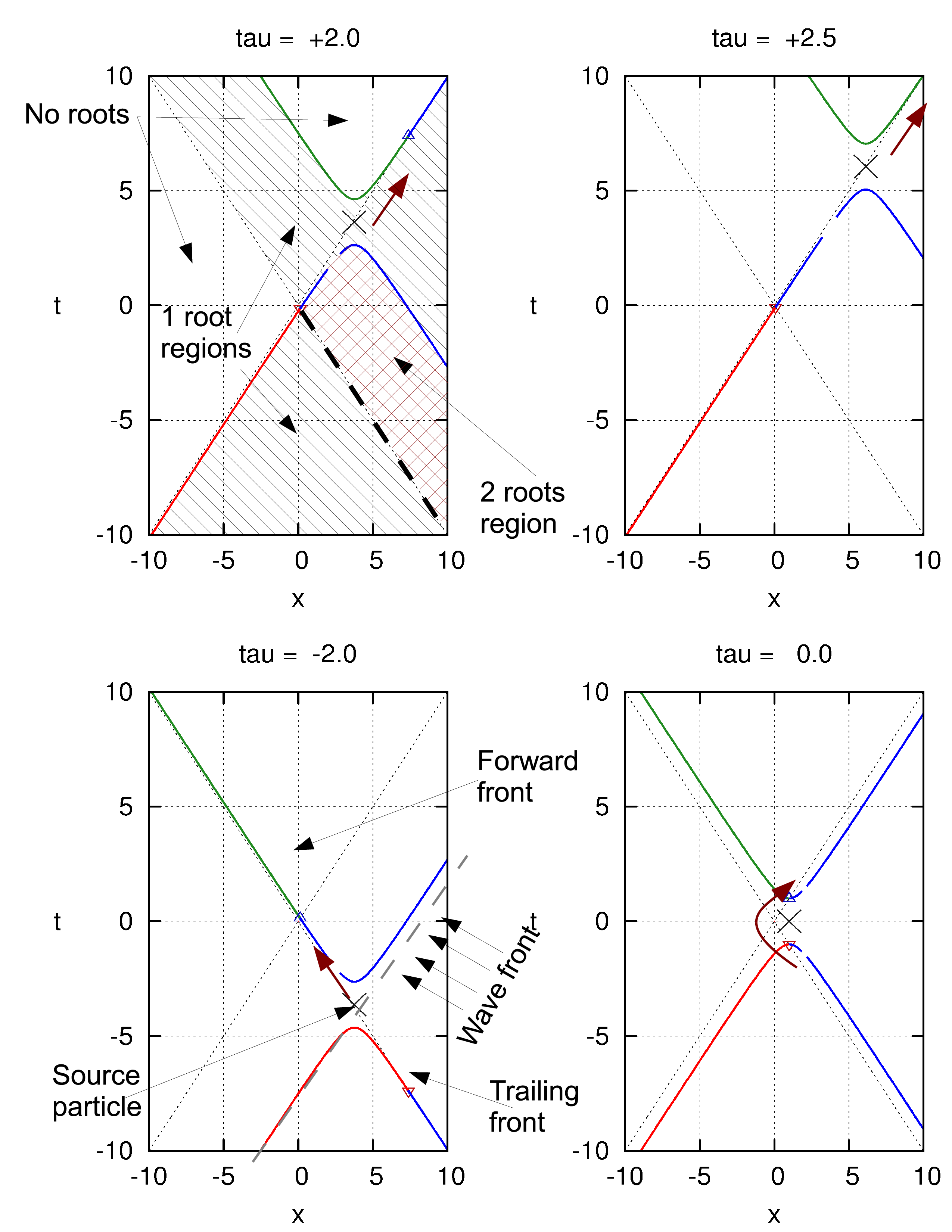
Figure 2: $xt$ location of roots $\tau^{\prime}_{0}(x,t)=\tau$. Each color shows the contour in a different quadrant (color online).

In figure 7 and 8, the values of the root are color plotted (online) on the $(x,t)$ plane for $\tau=-8$ and $\tau=-1.5$, respectively.

Even though it is not possible to extract a formal closed-form solution $\tau^{\prime}_{0}(x,t,\rho,\tau)$ such that $R(\tau^{\prime}_{0})=0$, one can easily plot contours of iso-root surface. In figure 2 the contour of the highest root $\tau^{\prime}_{0}=\tau$, is shown, for various values of $\tau$, and it has a special significance: it is the most advanced surface observable at a given $\tau$.

Clearly, an iso-root contour is a 2-sided hyperbola which center is the source particle itself at time $\tau$. This can be shown analytically as $R(\tau^{\prime})$ remains form invariant if $x\to x\cosh\alpha+t\sinh\alpha$, $t\to x\sinh\alpha+t\cosh\alpha$ and $\tau^{\prime}\to\tau^{\prime}-\alpha$, which clearly follows the hyperbolic motion of the source particle.

Several features can be observed in the iso-root plot, where we are using figure 2 as a reference:

• The two-sided hyperbola is due to the fact that there are 2 contours with the same root value.

• The lower side is the t-advanced front, at it appears for $t<z^{0}(\tau)$. The upper side is then clearly the t-retarded front.

• At $\tau\ll 0$, the lower-side hyperbola forms a trailing front behind the particle. This is clearly visible in figure 7.

• For the same $\tau\ll 0$, the upper-side hyperbola forms an advanced front, which approaches the $x=-t$ asymptotically. This advanced front is completely missing in figure 7, due to the very coarse resolution, whereas it is clearly visible in the finer resolution figure 8.

• When $\tau\gg 0$, the particle changes its asymptotic direction along the $x=t$ line, and the trailing and advanced fronts shift similarly from along the $x=-t$ to the $x=t$ lines.

• Each contour of the hyperbola has a half that is asymptotically parallel to the particle’s motion, and a half that is asymptotically orthogonal to it. The halves are exchanged as the particle crosses the $t=0$ line at $\tau=0$.

• For $\tau\ll 0$, the $x=-t$ line behind the particle, starting from the trailing front, is the location of a very high-field value. Similarly, for $\tau\gg 0$ the line $x=t$ in front of the particle, ending at the advanced front, is also a location of high field value.

  This can be easily seen by inspecting $\dot{R}(\tau^{\prime}_{0})$ along the $x=\pm t$ lines:

  $$\dot{R}_{\pm}(\tau^{\prime}) \equiv\dot{R}(\tau^{\prime})\Big{|}_{x=\pm t}=2(\tau-\tau^{\prime})\mp(x\mp t)e^{\mp\tau^{\prime}}$$

  Clearly, for roots $0<\tau-\tau^{\prime}_{0}\ll 1$, we have

  $$|\dot{R}_{\pm}(\tau^{\prime}_{0}\approx\tau)| \approx 2xe^{-|\tau|}$$

  Therefore, the fields diverge as $1/\dot{R}_{\pm}(\tau^{\prime}_{0})$.

• Quadrant I is the only quadrant where eventually, every point would covered by two roots of $\tau^{\prime}_{0}$. The region in quadrant I between the upper and lower sides of the hyperbola is where a single root $\tau^{\prime}_{0}$ exists. The region below the lower side of the hyperbola is where two roots exist.

  In quadrant IV, the region below the same side of the hyperbola has a single root.

  Thus, when crossing the line $x=-t$ below the lower-side of the hyperbola, moving from quadrant IV to quadrant I, the number of roots bifurcates from $1$ to $2$ roots, which can be seen in figure 3.

  As $\tau$ progresses, the doubly covered region (red in 3) continues to propagate into quadrant I, trailing the particle.

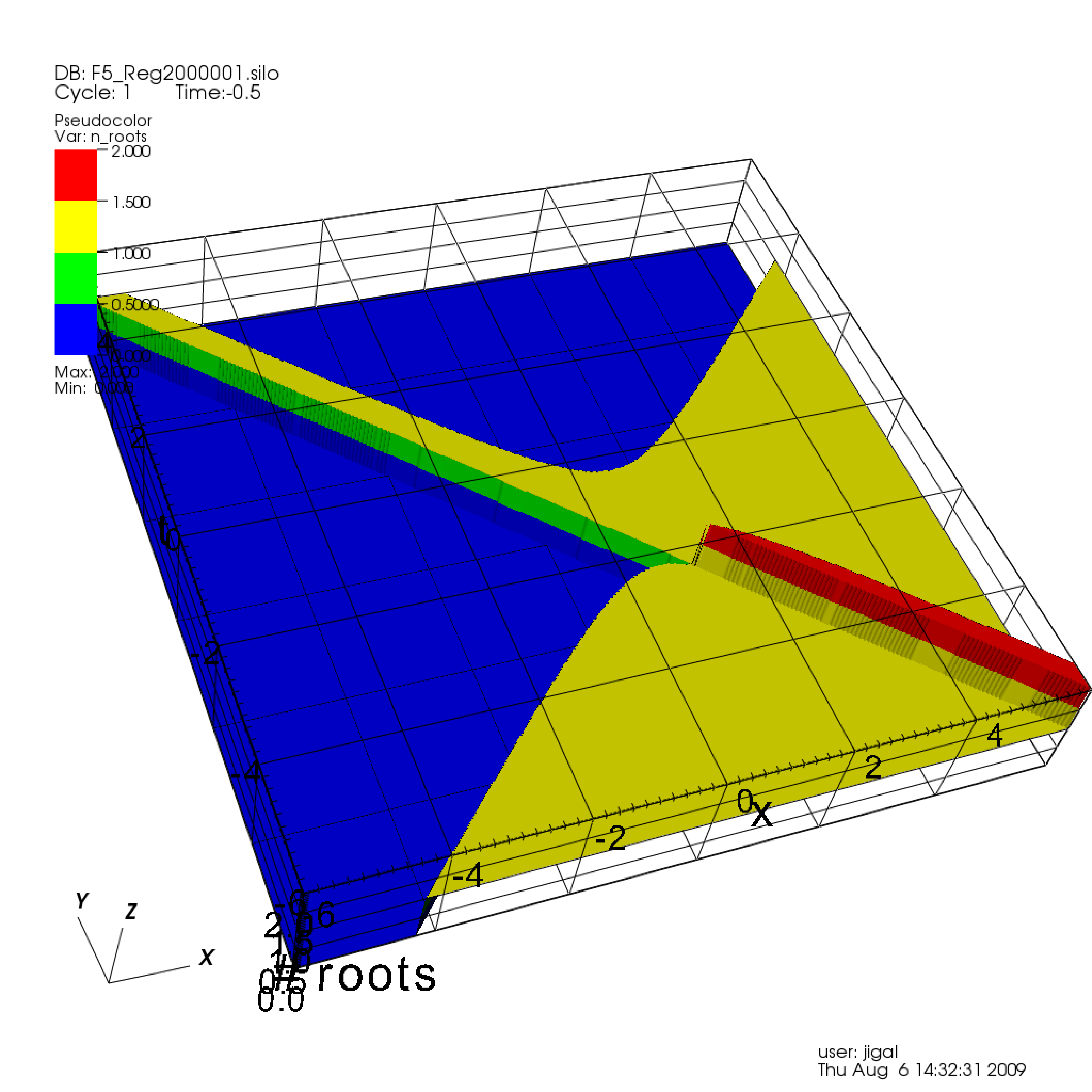
Figure 3: Number of roots at $\tau=-0.5$ (color online)

Notably, the $\tau^{\prime}$ support of the Green-function is different in each quadrant. In quadrant IV, the integration takes place from $(\tau^{\prime}_{0},\tau)$, in II from $(-\infty,\tau^{\prime}_{0})$ and in I it bifurcates to two ranges, from $(-\infty,{\tau^{\prime}}_{0}^{(1)})$ and $({\tau^{\prime}}_{0}^{(2)},\tau)$ where the history ${\tau^{\prime}}_{0}^{(1)}\leq\tau^{\prime}\leq{\tau^{\prime}}_{0}^{(2)}$ remains outside the domain of influence.

For points outside the characteristic $x=\pm t$, the root landscape $\tau^{\prime}_{0}(x,t,\tau)$ changes little when $\tau-\tau^{\prime}_{0}=h>O(g^{-1})$, and once a point $(x,t)$ is inside the past 5D light cone ($\tau^{\prime}_{0}\leq\tau$), its field value remains almost constant once $h=\tau-\tau^{\prime}_{0}>O(g^{-1})$.

In figure 5, a logarithmic color plot of the field $|f^{x\rho}|$ is given for $\tau=-8$. The location of the source and the direction of motion are depicted. Notably, the field is $0$ on the $x=-t$ line up to $x=-t=\frac{1}{2}(\rho^{2}+1)e^{-\tau}\approx 2981$. Behind the particle there is the trailing front. As the trailing front crosses the $x=-t$ line, the fields values there get very high due to $|\dot{R}_{\pm}(\tau^{\prime}_{0})|\ll 1$ along these lines.

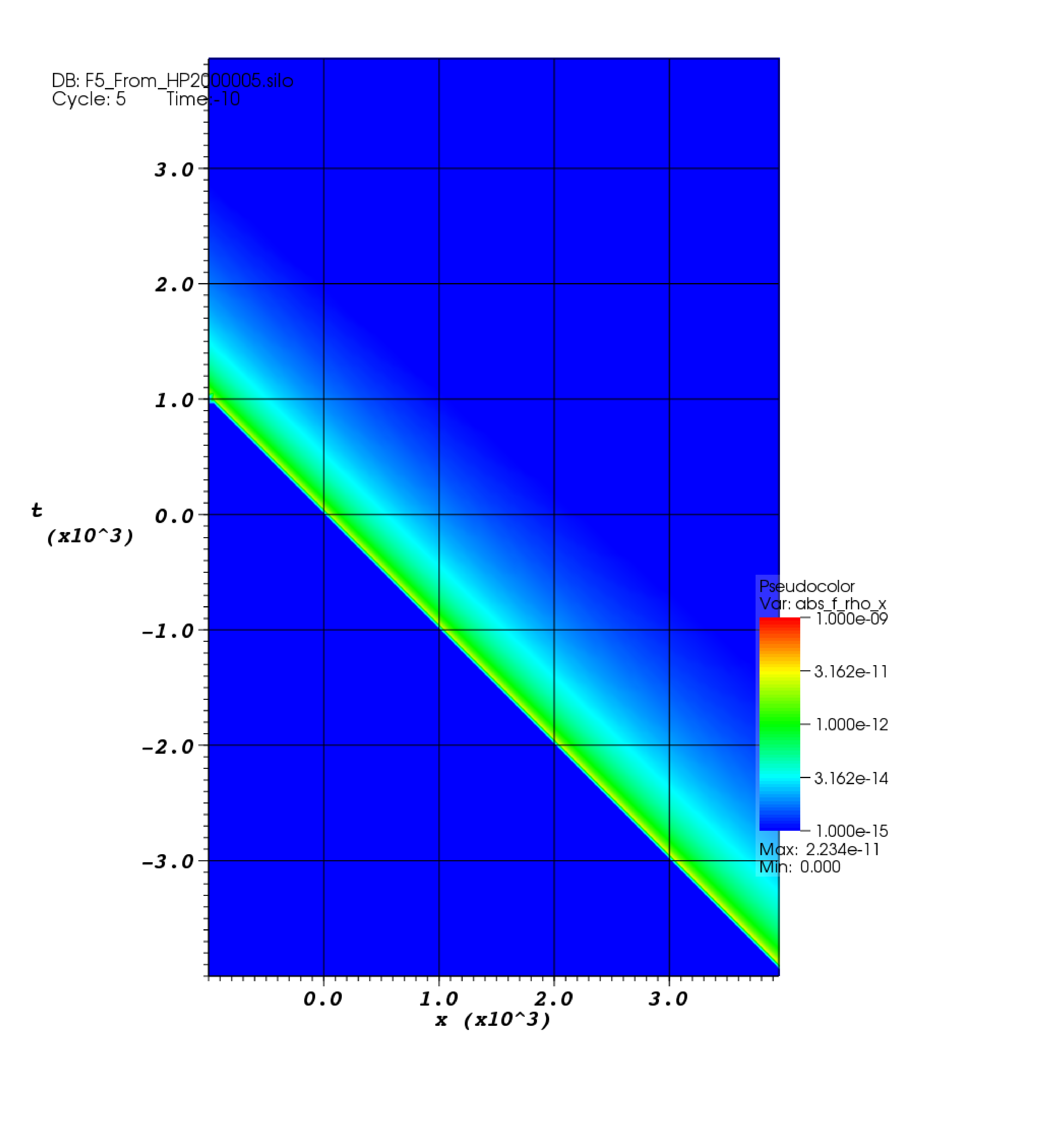
Figure 4: Logarithmic color plot of $|f^{x\rho}|$ at $\tau=-10$, $\rho=1$. The source particle is not visible in this spacetime patch (color online).

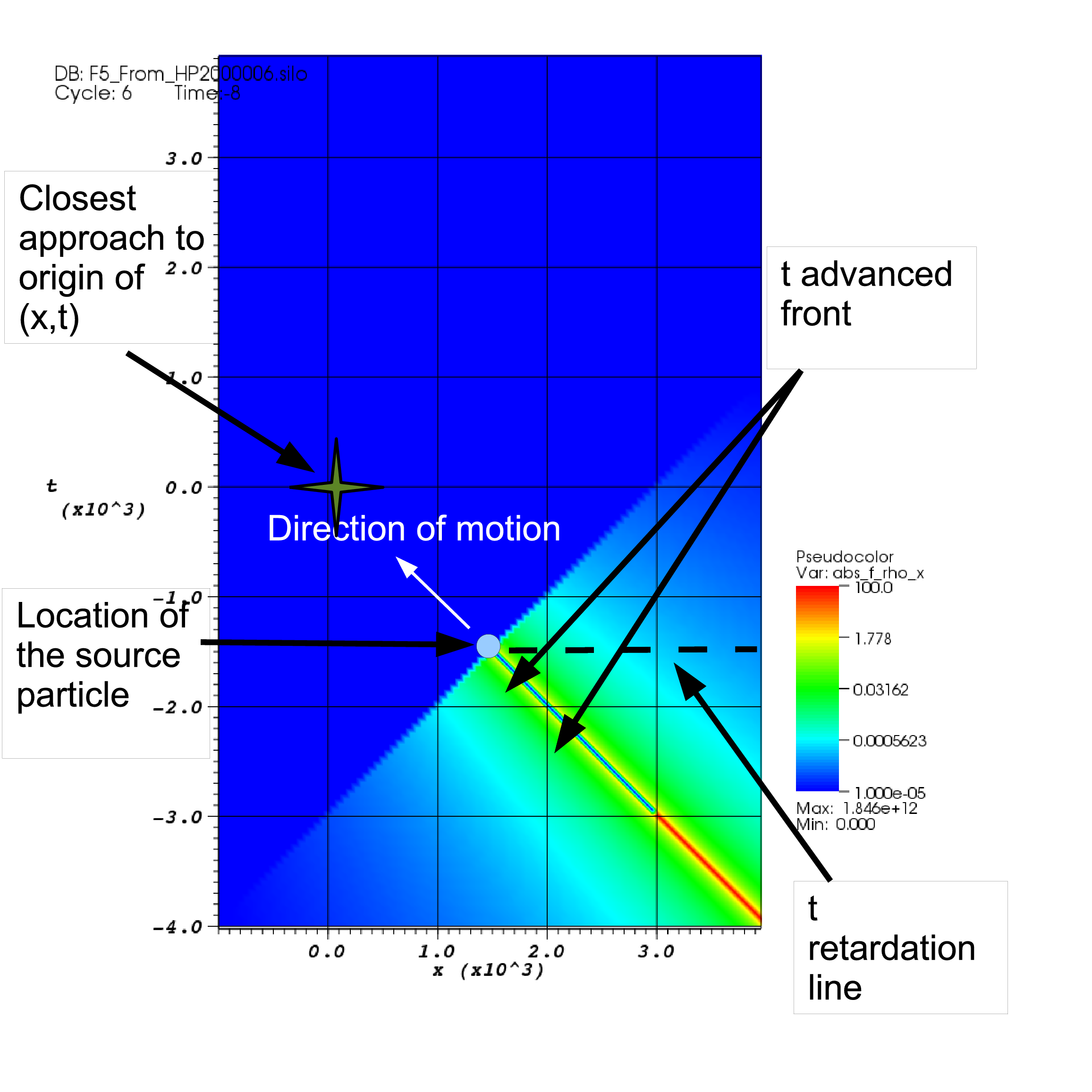
Figure 5: Logarithmic color plot of $|f^{x\rho}|$ at $\tau=-8$, $\rho=1$. The position source particle is shown (color online).

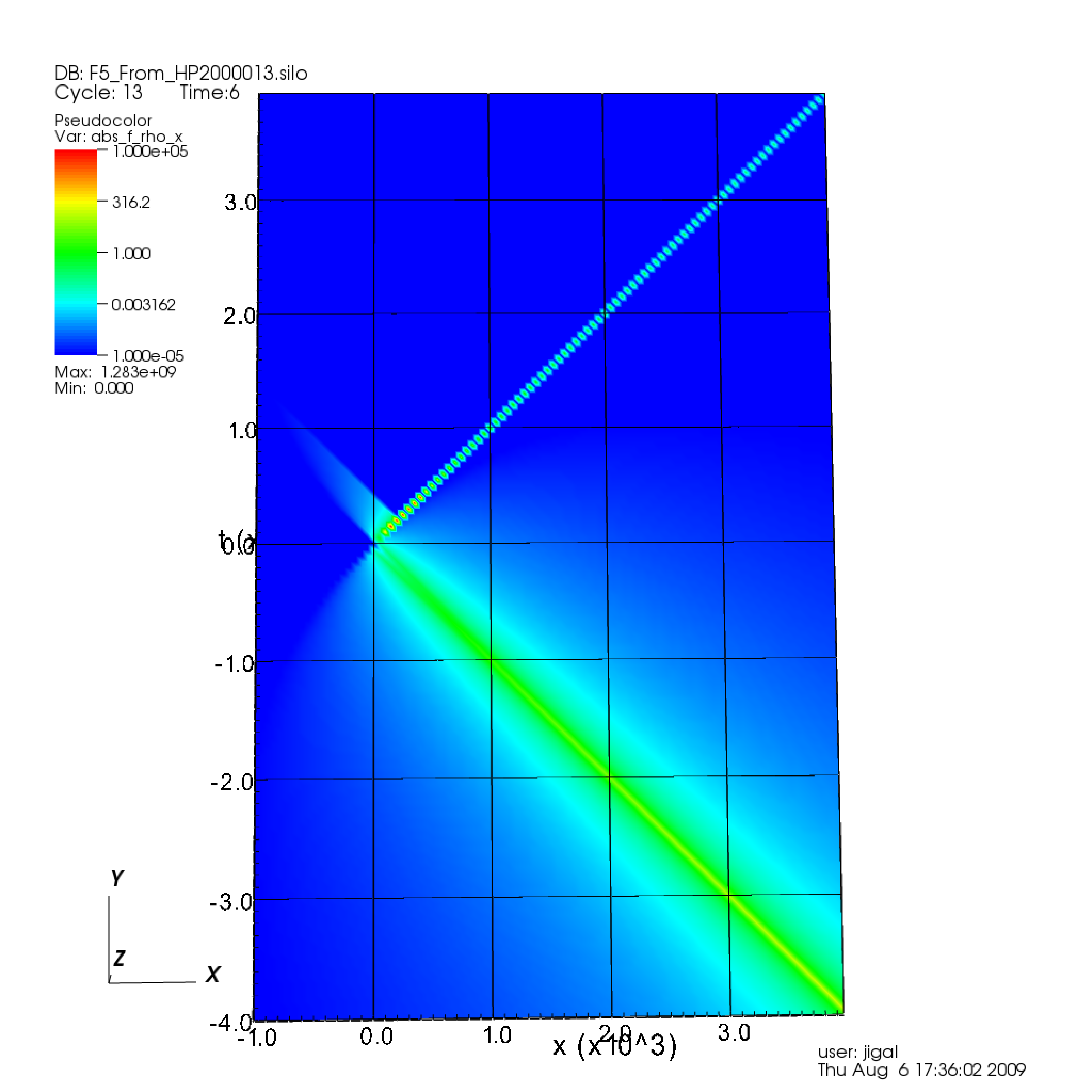
Figure 6: Logarithmic color plot of $|f^{x\rho}|$ at $\tau=6$ (color online).

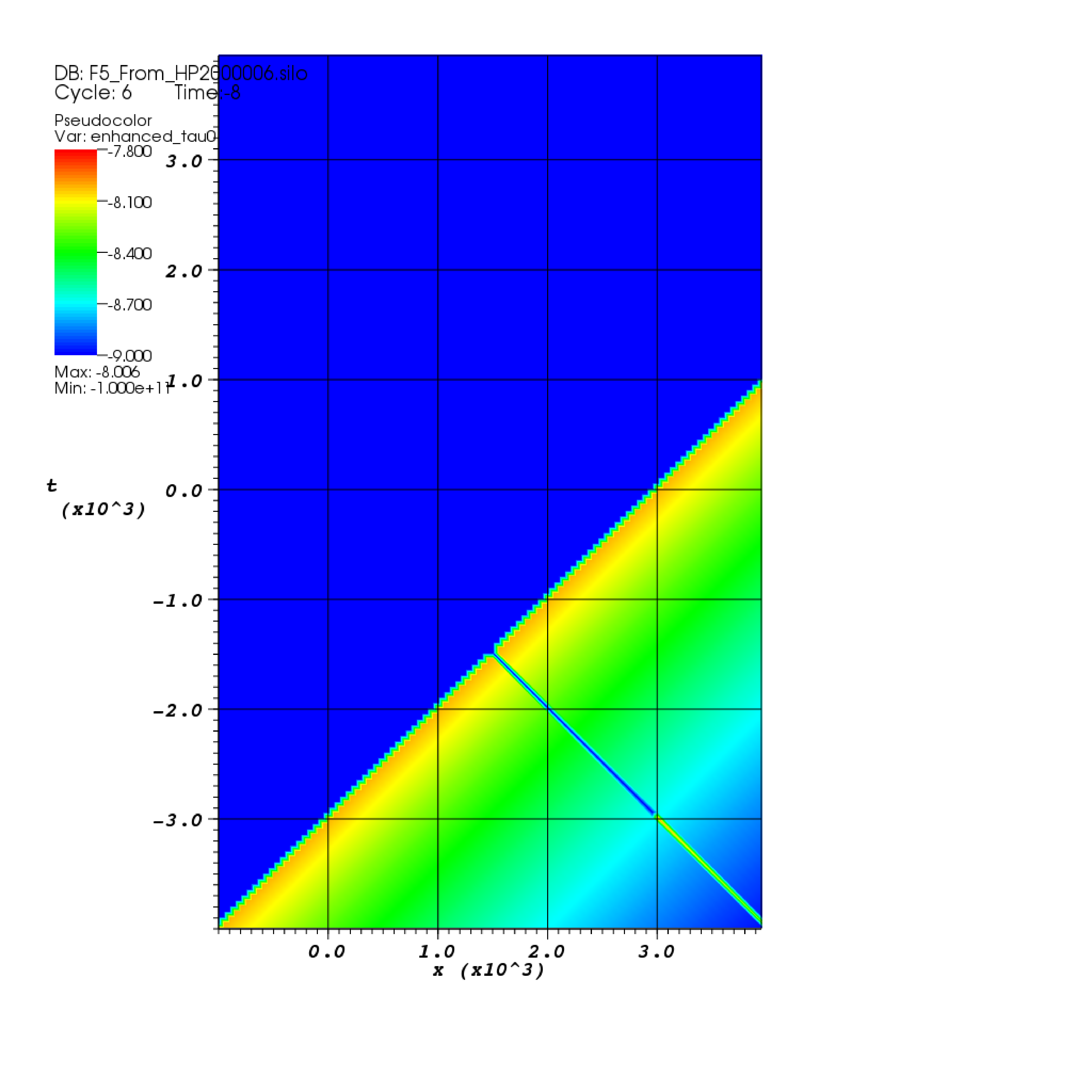
Figure 7: Linear plot of the root $\tau^{\prime}_{0}(x,t)$ obeying $R(\tau^{\prime}_{0})=0$, at $\tau=-8$. Upper part (blue color online) denotes areas where no root exists.

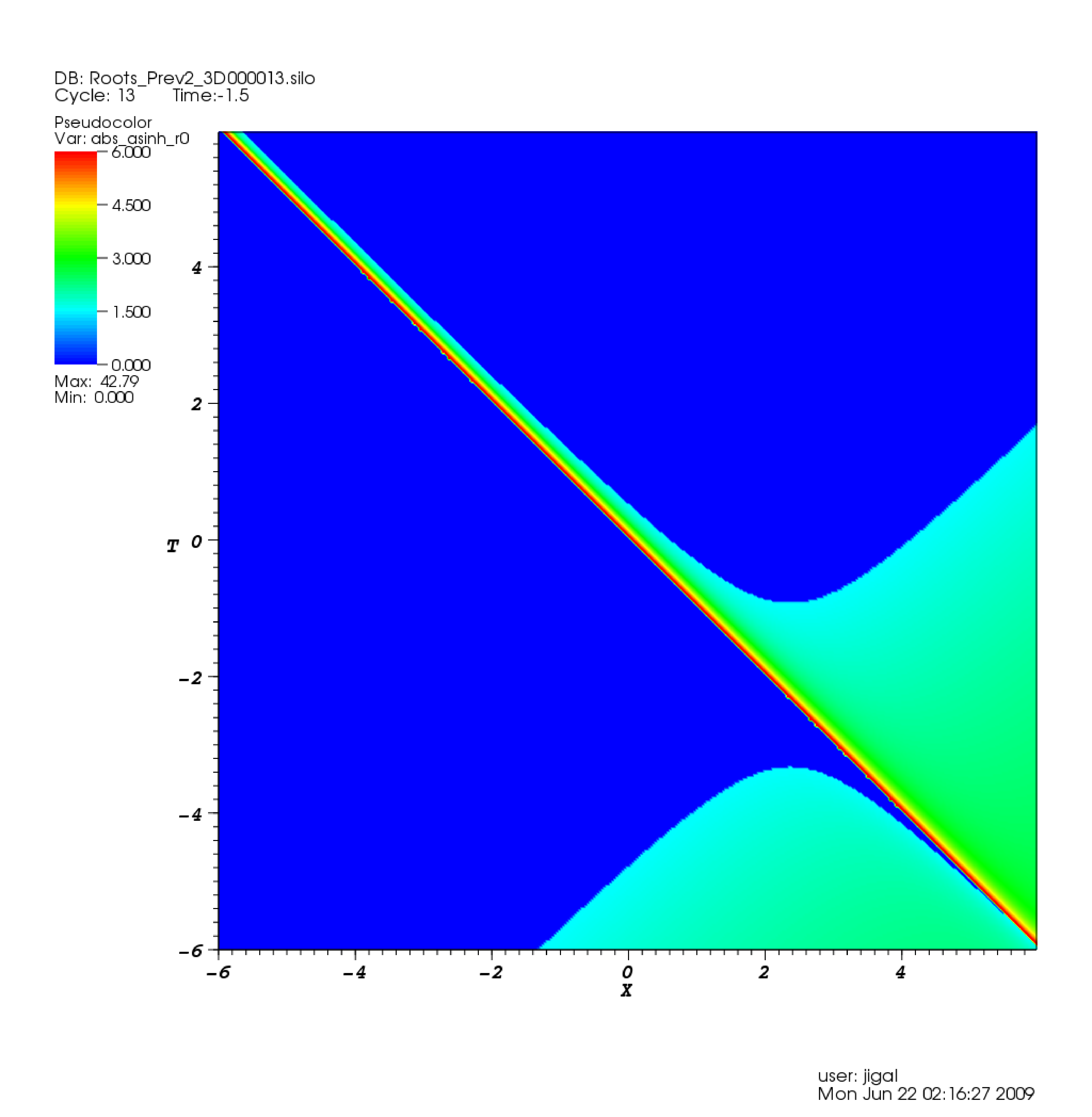
Figure 8: Same linear plot of the root $\tau^{\prime}_{0}(x,t)$ at much smaller scale, taken at $\tau=-1.5$ (color online).

5.4 Maxwell fields

For comparison, a logarithmic plot of the Maxwell field $|H_{\phi}|=|f_{x\rho}|$ as given by [39]:

$$H_{\phi} =\dfrac{8eg^{-2}\rho t}{\left[\left(g^{-2}-\rho^{2}+t^{2}-x^{2}\right)^{2}+4g^{-2}\rho^{2}\right]^{3/2}}$$ (69)

is shown in 9, using the same $(x,t)$ plane view and $\rho=1$ distance off the plane of motion (and the same relatively low resolution)

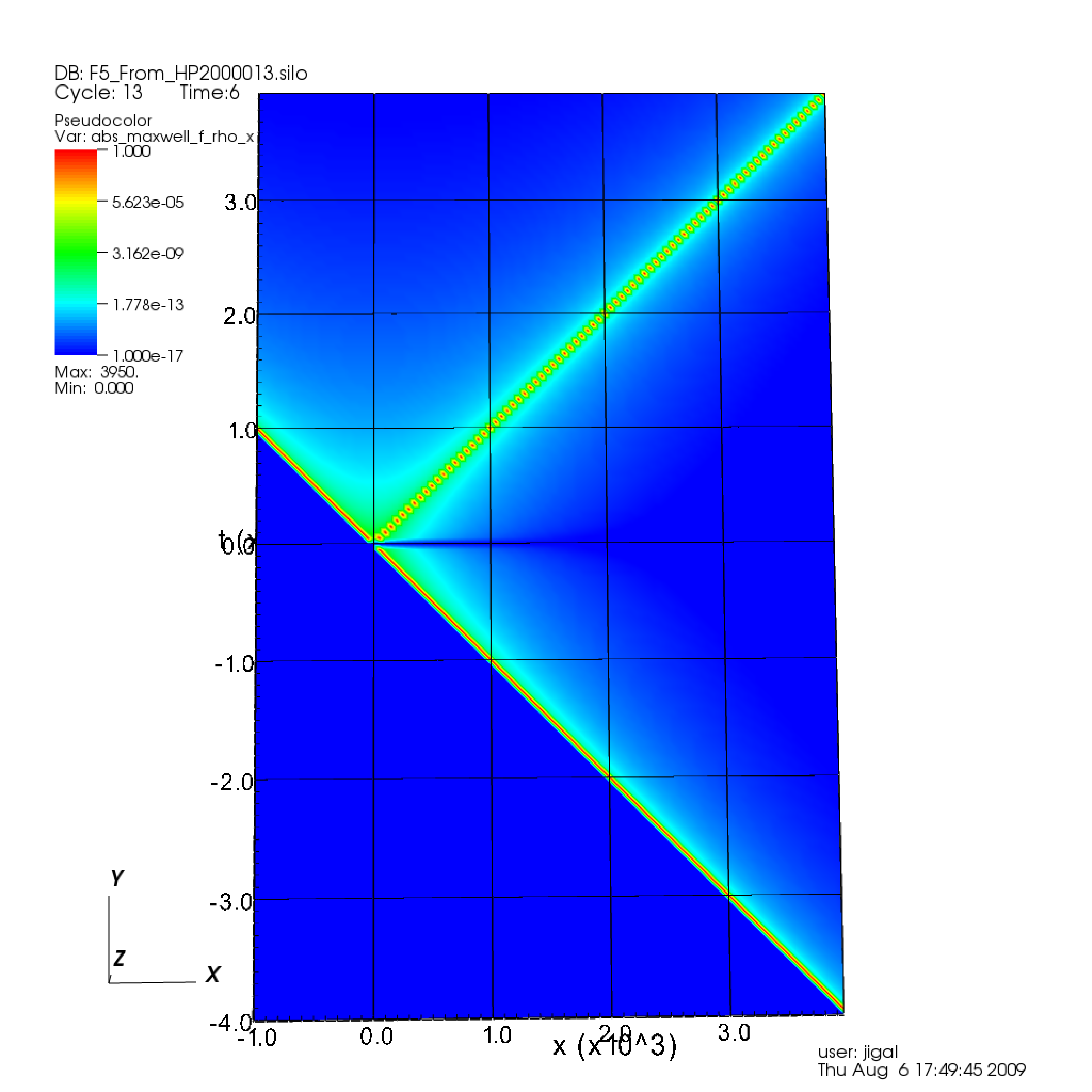
Figure 9: Maxwell $|H_{\phi}|=|f_{\rho x}|$ due to a uniformly accelerated source, to the same scale as figure 5 (color online)

The field shown is evaluated in the region denoted by Einstein retardation $x+t\geq 0$, i.e., only quadrants I and II have non-zero field. The 5D pre-Maxwell offshell fields, on the other hands, exhibit non-zero fields in quadrant IV as well, which are the source of the advanced fields (along with quadrant I).

5.5 Interpretation

In the 5D plots of the fields given in figures 6 ,5 and 4, the fields show a pattern which shares similarity with the Maxwell field as plotted in 9, in the sense that both show similar development up the $x=-t$. As the particle decelerates along the $x=-t$ axis, the field at the $x=-t$ plane is asymptotically infinite, as it is a buildup of an asymptotically null (in the 4D sense) particle in the infinite $\tau$-past. However, the field builds up on the negative side of $x$ as well, even though the source particle never visits it. As the source particle reverses its $x$-velocity at $\tau=0$, the field begins to buildup along the $x=+t$ surface.

A distinct character of the 5D fields is the $\tau$-motion in the $(x,t)$ plane, whereas clearly, the Maxwell-Einstein fields, as shown in figure 9, are essentially $\tau$-static.

A test particle in the $(x,t)$ plane, would in fact, correlate locally with the field at $(x,t)$ at the same $\tau$, by coupling to the generalized Lorentz force (17). In this sense, the test particle (or any other type of observer) sees a dynamic spacetime field. We shall study in a succeeding article, the motion of test particles in the fields that we have investigated.

Furthermore, as seen in figure 2, the double sided hyperbola is in fact strongly related to the fact the Green-functions are $\tau$-retarded and not $t$-retarded, as is the normal case in Maxwell fields. The $\tau$-retarded fields are, in fact, the average value of $t$-retarded and $t$-advanced fields. The lower-side hyperbola in figure 2 is in fact, the wave-front of the $t$-advanced field part, and the upper-side hyperbola is wave-front of the $t$-retarded part.

6 Summary and Conclusions

In order to solve simple problems in 5D off-shell electrodynamics, $\tau$ retarded Green-Functions (GF’s) were necessary, and these were derived using analytic continuation of Nozaki’s result [26], applicable both in $O(4,1)$ and $O(3,2)$ spacetime signature.

The machinery was then applied to a configuration studied long ago in the context of Maxwell electrodynamics, the radiation of a uniformly accelerated point source, which has generated decades of debate and though seemingly simple, has elucidated many important fundamental aspects on the nature of radiation.

However, we note that the vanishing of radiation reaction term $\Gamma^{\mu}_{\text{rr}}$ in the equation of motion of the source particle in Maxwell-Einstein electrodynamics does not occur in 5D off-shell electrodynamics.

The reason is the support of the GF is on the entire $\tau$ history of the source particle. Indeed, a full account of the off-shell fields in the equation of motion of the source particle is given by

$$M\ddot{x}^{\mu} =q\dot{x}^{\alpha}(\tau)f^{\mu}_{\,\,\,\alpha,\text{ext}}(x(\tau),\tau)+$$

$$\qquad+\dfrac{3\sigma_{5}q^{2}}{8\pi^{2}}\dot{x}^{\alpha}(\tau)\mathcal{R}\int_{-\infty}^{\tau}\dfrac{\theta(R(\tau^{\prime}))}{R^{5/2}(\tau^{\prime})}\left[\dot{x}^{\mu}(\tau^{\prime})\partial_{\alpha}R(\tau^{\prime})-\dot{x}_{\alpha}(\tau^{\prime})\partial^{\mu}R(\tau^{\prime})\right]\mathop{}\!\mathrm{d}\tau^{\prime}$$ (70)

where $R(\tau^{\prime})$ is identical to (65), except that it now relates the same source particle at different $\tau$ times:

$$R(\tau^{\prime}) =-\sigma_{5}(x(\tau)-x(\tau^{\prime}))^{2}$$ (71)

It can easily be shown that the radiation reaction term in (70) does not vanish for the case of uniform acceleration, though it does vanish identically for uniform motion, which suggests that there is radiation reaction force in the accelerating case.

Generally, the $\tau$-retarded fields can further be decomposed to the sum of $t$-retarded and $t$-advanced fields. Locally, a test particle interacts with both these fields.

Appendix A Canonical regularization of divergent integrals

In this section we provide a short overview of the regularization method described in Gel’fand [13].

The function $x^{\lambda}_{+}\equiv\theta(x)x^{\lambda}$ is non-zero for positive $x$, where $\theta(x)$ is the step-function. When acting on a smooth bounded function $\phi(x)$

$$\left(x_{+}^{\lambda},\phi(x)\right) =\int_{0}^{\infty}x^{\lambda}\phi(x)\,\mathop{}\!\mathrm{d}x$$

is well defined for $\Re\lambda>-1$. On the other hand, the expression can be rewritten as

$$\left(x_{+}^{\lambda},\phi(x)\right) =\int_{0}^{b}x^{\lambda}\left[\phi(x)-\sum_{j=0}^{m}\dfrac{\phi^{(j)}(0)}{j!}x^{j}\right]\mathop{}\!\mathrm{d}x+\sum_{j=0}^{m}\dfrac{\phi^{(j)}(0)}{j!(\lambda+j+1)}b^{\lambda+j+1}+$$

$$\qquad+\int_{b}^{\infty}x^{\lambda}\phi(x)\,\mathop{}\!\mathrm{d}x$$ (72)

where the right-hand-side is well defined for $\{\Re\lambda>-m\}\cap\{\lambda\neq-1,-2,\}$.

This suggests that, as a generalized function, $x_{+}^{\lambda}$ can be defined by its action on any smooth bounded function $\phi(x)$, as given by (A). The result is a function of $\lambda$ defined for all $\Re\lambda>-m$ except at $\lambda=-1,-2,\ldots-m+1$ where it has simple poles with residues $\dfrac{\phi^{(j)}(0)}{j!}$. This suggests that $x_{+}^{\lambda}$ itself is a generalized function with simple poles given by

$$\text{Res }x_{+}^{\lambda}\Big{|}_{\lambda=-n} =(-1)^{n}\dfrac{\delta^{(n)}(x)}{n!}$$

Similarly, given 2 smooth functions, $\phi(x)$ and $R(x)$, we are seeking a regularized solution for

$$\left(R_{+}^{-\lambda}(x),\phi(x)\right) =\int_{a}^{b}\dfrac{\phi(x)}{R^{\lambda}(x)}\mathop{}\!\mathrm{d}x$$ (73)

where, $a$ is defined by $R(a)=0$, and $R(x)>0$ for $x\in(a,b)$. One can select $c$ such that $a<c<b$ and $\dot{R}(x)\equiv dR/dx\neq 0$ for all $x\in[a,c]$. Setting $h=c-a>0$, we find

$$\left(R_{+}^{-\lambda}(x),\phi(x)\right) =\int_{a}^{a+h}\dfrac{\phi(x)}{R^{\lambda}(x)}\mathop{}\!\mathrm{d}x+\int_{a+h}^{b}\dfrac{\phi(x)}{R^{\lambda}(x)}\mathop{}\!\mathrm{d}x$$ (74)

$$=\int_{0}^{R_{h}}\dfrac{\phi(x(R))}{R^{\lambda}}\dfrac{dR}{\dot{R}(x(R))}+\int_{a+h}^{b}\dfrac{\phi(x)}{R^{\lambda}(x)}\mathop{}\!\mathrm{d}x$$ (75)

where the first integral in $x$ was transformed to an integral in $R$, since $dR>0$ in the interval $(a,a+h)$. One can then proceed with the regularization as given in (A)

$$\left(R_{+}^{-\lambda}(x),\phi(x)\right) =\int_{0}^{R_{h}}R^{-\lambda}\left[\dfrac{\phi(R)}{\dot{R}(R)}-\sum_{j=0}^{m}\dfrac{R^{j}}{j!}\dfrac{\mathop{}\!\mathrm{d}^{j}}{\mathop{}\!\mathrm{d}R^{j}}\left(\dfrac{\phi(a)}{\dot{R}(a)}\right)\right]\mathop{}\!\mathrm{d}R+$$

$$\qquad+\sum_{j=0}^{m}\dfrac{R^{j-\lambda+1}_{h}}{(j-\lambda+1)j!}\dfrac{\mathop{}\!\mathrm{d}^{j}}{\mathop{}\!\mathrm{d}R^{j}}\left(\dfrac{\phi(a)}{\dot{R}(a)}\right)+\int_{a+h}^{b}\dfrac{\phi(x)}{R^{\lambda}(x)}\mathop{}\!\mathrm{d}x$$

where $R_{h}=R(a+h)$. Once the regularized integral is given in $R$, it can be transformed back to $x$:

$$\dfrac{d}{dR} =\dfrac{\mathop{}\!\mathrm{d}x}{\mathop{}\!\mathrm{d}R}\dfrac{\mathop{}\!\mathrm{d}}{\mathop{}\!\mathrm{d}x}=\dfrac{1}{\dot{R}(x)}\dfrac{\mathop{}\!\mathrm{d}}{\mathop{}\!\mathrm{d}x}$$

Thus:

$$\left(R_{+}^{-\lambda}(x),\phi(x)\right) =\int_{a}^{a+h}R^{-\lambda}(x)\left[\phi(x)-\sum_{j=0}^{m}\dfrac{R^{j}(x)}{j!}\left(\dfrac{1}{\dot{R}(x)}\dfrac{d}{dx}\right)^{j}\left(\dfrac{\phi(a)}{\dot{R}(a)}\right)\right]\mathop{}\!\mathrm{d}x+$$

$$\qquad+\sum_{j=0}^{m}\dfrac{R^{j-\lambda+1}_{h}}{(j-\lambda+1)j!}\left(\dfrac{1}{\dot{R}(x)}\dfrac{\mathop{}\!\mathrm{d}}{\mathop{}\!\mathrm{d}x}\right)^{j}\left(\dfrac{\phi(a)}{\dot{R}(a)}\right)+\int_{a+h}^{b}\dfrac{\phi(x)}{R^{\lambda}(x)}\mathop{}\!\mathrm{d}x$$

from which the regularization (3.3) can readily be obtained by setting $\lambda=5/2$ and $m=1$.

Appendix B Derivation of the $\tau$ retarded Green Function

The derivation of $\tau$ retarded Green-functions was made with essentially the same method as Y. Nozaki [26], which defined a generalized Riemann-Liouville type integrodifferential operator for ultrahyperbolic spaces, itself a generalization of an earlier monumental work by M. Riesz [31, 32].

Following Nozaki [26], we shall show $L^{\alpha}$ can generate the fundamental solution of the $\Delta_{p,q}$ wave-operator with retardation in $x_{m}$.

There are three stages involved in order to establish the desired Green-Function is indeed the kernel of the operator $L^{\alpha}$. This is the sibject of the next paragraphs.

Normalization constant $N_{m}(\alpha)$

The first step is to establish $L^{\alpha}$ by finding $N_{m}(\alpha)$, the normalization constant, such that

$$(L^{\alpha}e^{x_{m}})(x) =e^{x_{m}}$$ (76)

This is akin to the Riemann-Liouville operator in one dimension

$$(I^{\alpha}e^{x})(x) =e^{x}=\dfrac{1}{\Gamma(\alpha)}\int_{-\infty}^{x}(x-y)^{\alpha-1}e^{y}\mathop{}\!\mathrm{d}y$$

which can easily be proven by changing variables to $u=x-y$.

Thus, we have:

$$(L^{\alpha}e^{x_{m}})(x) =\dfrac{1}{N_{m}(\alpha)}\int_{\mathcal{D}_{x}}r^{\alpha-m}(x-y)e^{y_{m}}\mathop{}\!\mathrm{d}^{m}y$$

Changing variables $y_{i}\to x_{i}-y_{i}$ we obtain:

$$(L^{\alpha}e^{x_{m}})(x) =\dfrac{1}{N_{m}(\alpha)}\int_{\mathcal{D}_{0}}r^{\alpha-m}(y)e^{x_{m}-y_{m}}\mathop{}\!\mathrm{d}^{m}y=\dfrac{e^{x_{m}}}{N_{m}(\alpha)}\int_{\mathcal{D}_{0}}r^{\alpha-m}(y)e^{-y_{m}}\mathop{}\!\mathrm{d}^{m}y$$

Making the substitution

$$s^{2} =\sum_{i=1}^{p}y_{i}^{2},\qquad t^{2}=\sum_{j=1}^{q}y_{p+j}^{2},\qquad r^{\alpha-m}(y)=(s^{2}-t^{2})^{(\alpha-m)/2}$$

$$\mathop{}\!\mathrm{d}^{m}y =s^{p-1}t^{q-1}\mathop{}\!\mathrm{d}s\mathop{}\!\mathrm{d}t\mathop{}\!\mathrm{d}\Omega_{p}\mathop{}\!\mathrm{d}\Omega_{q},\qquad y_{m}=t\cos(\theta_{q-1})$$

we find:

$$(L^{\alpha}e^{x_{m}})(x) =\dfrac{e^{x_{m}}}{N_{m}(\alpha)}\int_{0}^{\infty}t^{q-1}\mathop{}\!\mathrm{d}q\int_{t}^{\infty}s^{p-1}\mathop{}\!\mathrm{d}s\int_{S^{p}}\mathop{}\!\mathrm{d}\Omega_{p}\int_{S^{q-1}}\mathop{}\!\mathrm{d}\Omega_{q-1}$$

$$\qquad\times\int_{0}^{\pi/2}\sin^{q-2}(\theta_{q-1})\mathop{}\!\mathrm{d}\theta_{q-1}(s^{2}-t^{2})^{(\alpha-m)/2}e^{-t\cos(\theta_{q-1})}$$

where $\theta_{q-1}$ is integrated from $0$ to $\pi/2$ signifying retardation in $x_{m}$. We begin with the integration over $s$, by changing variables to $w(s)=t^{2}/s^{2}$ which leads to

$$\int_{t}^{\infty}s^{p-1} (s^{2}-t^{2})^{(\alpha-m)/2}\mathop{}\!\mathrm{d}s=$$

$$=\dfrac{1}{2}t^{1+2(p-1)/2}t^{2(\alpha-m)/2}\int_{0}^{1}w^{-(p-1)/2-(\alpha-m)/2+3/2}(1-w)^{(\alpha-m)/2}\mathop{}\!\mathrm{d}w$$

$$=\dfrac{1}{2}t^{\alpha-m+p}\int_{0}^{1}w^{(m-p-\alpha)/2-1}(1-w)^{(\alpha-m)/2+1-1}\mathop{}\!\mathrm{d}w$$

$$=t^{\alpha-m+p}B\left(\dfrac{m-p-\alpha}{2},\dfrac{\alpha-m}{2}+1\right)\qquad\qquad\text{where $B(x,y)$ is the \emph{Beta function}.}$$

$$=t^{\alpha-q}\dfrac{\Gamma\left(\dfrac{q-\alpha}{2}\right)\Gamma\left(\dfrac{\alpha-m}{2}+1\right)}{\Gamma\left(1-\dfrac{p}{2}\right)}$$

Thus, $L^{\alpha}e^{x_{m}}$ takes the form

$$(L^{\alpha}e^{x_{m}})(x) =\dfrac{e^{x_{m}}}{N_{m}(\alpha)}\dfrac{\Gamma\left(\dfrac{q-\alpha}{2}\right)\Gamma\left(\dfrac{\alpha-m}{2}+1\right)}{\Gamma\left(1-\dfrac{p}{2}\right)}\int_{S^{p}}d\Omega_{p}\int_{S^{q-1}}d\Omega_{q-1}$$

$$\qquad\times\int_{0}^{\pi/2}\sin^{q-2}(\theta_{q-1})\mathop{}\!\mathrm{d}\theta_{q-1}\int_{0}^{\infty}t^{q-1}t^{\alpha-q}e^{-t\cos(\theta_{q-1})}\mathop{}\!\mathrm{d}t$$

Integration over $S^{p}$ has the usual result $2\pi^{p/2}/\Gamma(p/2)$, and a similar result for the integration over $S^{q-1}$. The $t$ integration is performed by making the substitution $w=t\cos(\theta_{q-1})$ (and carefully noting that $\cos\theta_{q-1}\geq 0$ in the range of integration):

$$\int_{0}^{\infty}t^{q-1} t^{\alpha-q}e^{-t\cos(\theta_{q-1})}\mathop{}\!\mathrm{d}t=\int_{0}^{\infty}t^{\alpha-1}e^{-t\cos(\theta_{q-1})}\mathop{}\!\mathrm{d}t$$

$$=\dfrac{1}{\cos(\theta_{q-1})}\int_{0}^{\infty}\left(\dfrac{w}{\cos(\theta_{q-1})}\right)^{\alpha-1}e^{-w}\mathop{}\!\mathrm{d}w$$

$$=\dfrac{1}{\cos^{1+\alpha-1}(\theta_{q-1})}\int_{0}^{\infty}w^{\alpha-1}e^{-w}\mathop{}\!\mathrm{d}w$$

$$=\dfrac{\Gamma(\alpha)}{\cos^{1+\alpha-1}(\theta_{q-1})}$$

Thus:

$$(L^{\alpha}e^{x_{m}})(x) =\dfrac{e^{x_{m}}}{N_{m}(\alpha)}\dfrac{\Gamma\left(\dfrac{q-\alpha}{2}\right)\Gamma\left(\dfrac{\alpha-m}{2}+1\right)}{\Gamma\left(1-\dfrac{p}{2}\right)}\dfrac{2\pi^{p/2}}{\Gamma(p/2)}\dfrac{2\pi^{(q-1)/2}}{\Gamma((q-1)/2)}\Gamma(\alpha)$$

$$\qquad\times\int_{0}^{\pi/2}\dfrac{\sin^{q-2}(\theta_{q-1})}{\cos^{\alpha}(\theta_{q-1})}\mathop{}\!\mathrm{d}\theta_{q-1}$$

where the $\theta_{q-1}$ integration can be taken by using the identity

$$B(a,b) =2\int_{0}^{\pi/2}\sin^{2a-1}(\theta)\cos^{2b-1}(\theta)\mathop{}\!\mathrm{d}\theta$$ (77)

Thus, one finally has

$$(L^{\alpha}e^{x_{m}})(x) =\dfrac{e^{x_{m}}}{N_{m}(\alpha)}\dfrac{\Gamma\left(\dfrac{q-\alpha}{2}\right)\Gamma\left(\dfrac{\alpha-m}{2}+1\right)}{\Gamma\left(1-\dfrac{p}{2}\right)}\dfrac{2\pi^{p/2}}{\Gamma(p/2)}\dfrac{2\pi^{(q-1)/2}}{\Gamma((q-1)/2)}\Gamma(\alpha)$$

$$\qquad\times\dfrac{1}{2}\dfrac{\Gamma\left(\dfrac{q-1}{2}\right)\Gamma\left(\dfrac{1-\alpha}{2}\right)}{\Gamma\left(\dfrac{q-\alpha}{2}\right)}$$

And since $L^{\alpha}e^{x_{m}}=e^{x_{m}}$ we find:

$$N_{m}(\alpha) =2\pi^{(m-3)/2}\Gamma(\alpha)\sin\left(\dfrac{p\pi}{2}\right)\Gamma\left(1-\dfrac{m-\alpha}{2}\right)\Gamma\left(1-\dfrac{\alpha}{2}\right)$$ (78)

which clearly coincides with (58).

Operation under the ultrahyperbolic d’Alembert operator

Writing

$$L^{\alpha}f =\int_{\mathcal{D^{\prime}}_{x}}\Phi_{\alpha}(x-y)f(y)\mathop{}\!\mathrm{d}^{m}y$$

where $\Phi_{\alpha}(x)=r^{\alpha-m}(x)/N_{m}(\alpha)$, we can evaluate the action of $\Delta\Phi_{\alpha}(x)$ directly:

$$\Delta\Phi_{\alpha}(x) =\dfrac{1}{N_{m}(\alpha)}\Delta r^{\alpha-m}(x)=\dfrac{1}{N_{m}(\alpha)}(\alpha-m)(\alpha-2)r^{\alpha-m-2}(x)$$

$$=\dfrac{N_{m}(\alpha-2)}{N_{m}(\alpha)}(\alpha-m)(\alpha-2)\Phi_{\alpha-2}(x)$$

Now:

$$\dfrac{N_{m}(\alpha-2)}{N_{m}(\alpha)} =\dfrac{\Gamma\left(\dfrac{\alpha-m}{2}\right)\Gamma\left(\dfrac{3-\alpha}{2}\right)\Gamma\left(\alpha-2\right)}{\Gamma\left(\dfrac{2+\alpha-m}{2}\right)\Gamma\left(\dfrac{1-\alpha}{2}\right)\Gamma\left(\alpha\right)}$$

$$=\dfrac{\Gamma\left(\dfrac{\alpha-m}{2}\right)\left[\left(\dfrac{1-\alpha}{2}\right)\Gamma\left(\dfrac{1-\alpha}{2}\right)\right]\Gamma\left(\alpha-2\right)}{\left[\left(\dfrac{\alpha-m}{2}\right)\Gamma\left(\dfrac{\alpha-m}{2}\right)\right]\Gamma\left(\dfrac{1-\alpha}{2}\right)\Big{[}(\alpha-2)(\alpha-1)\Gamma\left(\alpha-2\right)\Big{]}}$$

$$=-\dfrac{1}{(\alpha-m)(\alpha-2)}$$

which immediately leads to

$$\Delta\Phi_{\alpha}(x) =-\Phi_{\alpha-2}(x)\Longrightarrow\Delta(L^{\alpha}f)(x)=(L^{\alpha-2}f)(x)$$ (79)

$L^{\alpha}$ near $\alpha\to 0$

In [26], it was shown that

$$\lim\limits_{\alpha\to 0^{+}}(J^{\alpha}f)(x) =f(x)\Longrightarrow\lim\limits_{\alpha\to 0^{+}}J^{\alpha}=\delta(x)$$ (80)

which was shown by extending the operation of $J^{\alpha}$ to include its advanced counterpart $\bar{J}^{\alpha}$. The same exact proof can also be established here by extending $L^{\alpha}$, which essentially produces the same operator $L^{\alpha}+\bar{L}^{\alpha}=J^{\alpha}+\bar{J}^{\alpha}$.

Therefore, one immediately has

$$\lim\limits_{\alpha\to 0^{+}}L^{\alpha} =\delta(x)$$ (81)

This means that the Green-Function is essentially $-\Phi_{2}(x)$, as

$$\Delta\Phi_{2}(x) =-\Phi_{0}(x)=-\delta(x)$$ (82)

as originally desired, leading to (59).

References

- [1] I. Aharonovich and L. P. Horwitz. Green functions for wave propagation on a five-dimensional manifold and the associated gauge fields generated by a uniformly moving point source. Journal of Mathematical Physics, 47(12):122902, 2006.
- [2] R. Arshansky and L. P. Horwitz. The quantum relativistic two-body bound state. i. the spectrum. Journal of Mathematical Physics, 30(1):66–80, 1989.
- [3] R. Arshansky and L. P. Horwitz. The quantum relativistic two-body bound state. ii. the induced representation of sl(2,c). Journal of Mathematical Physics, 30(2):380–392, 1989.
- [4] R. Arshansky and L. P. Horwitz. Relativistic potential scattering and phase shift analysis. Journal of Mathematical Physics, 30(1):213–218, 1989.
- [5] David H. Bailey, Hida Yozo, Xiaoye S. Li, and Brandon Thompson. ARPREC: An arbitrary precision computation package. Lawrence Berkeley National Laboratory, Paper LBNL-53651, 2002.
- [6] H. Bondi and T. Gold. The Field of a Uniformly Accelerated Charge, with Special Reference to the Problem of Gravitational Acceleration. Proceedings of the Royal Society of London. Series A, Mathematical and Physical Sciences (1934-1990), 229:416–424, 1955.
- [7] Max Born. The theory of the rigid electron in the kinetics of the relativity principle (from german). Annalen der Physik, 335:1–56, 1909.
- [8] David G. Boulware. Radiation from a uniformly accelerated charge. Annals of Physics, 124(1):169–188, January 1980.
- [9] L. Burakovsky, L. P. Horwitz, and W. C. Schieve. New relativistic high-temperature bose-einstein condensation. Phys. Rev. D, 54(6):4029–4038, Sep 1996, hep-th/9604039.
- [10] P. A. M. Dirac. Classical theory of radiating electrons. Proceedings of the Royal Society of London. Series A, Mathematical and Physical Sciences (1934-1990), 167(929):148–169, August 1938.
- [11] Thomas Fulton and Fritz Rohrlich. Classical radiation from a uniformly accelerated charge. Annals of Physics, 9:499–517, 1960.
- [12] Gal’tsov and V. Dmitri. Radiation reaction in various dimensions. Phys. Rev. D, 66(2):025016, July 2002, hep-th/0112110.
- [13] I. M. Gel’fand and G. E. Shilov. Generalized Functions, Properties and Operations, volume 1 of Generalized Functions. Academic Press, 1964. Translated from Russian.
- [14] V. L. Ginzburg. Radiation reaction and friction force in uniformly accelerated motion of a charge. Soviet Physics Uspekhi, 12(4):565–574, July-August 1970.
- [15] Brian J. Gough. GNU Scientific Library Reference Manual. Network Theory Ltd., 3rd edition, 2009.
- [16] Metin Gurses and Ozgur Sarioglu. Lienard-wiechert potentials in even dimensions. Journal of Mathematical Physics, 44:4672, 2003.
- [17] Amos Harpaz and Noam Soker. Radiation from a uniformly accelerated charge. Gen. Rel. Grav., 30:1217–1227, 1998, gr-qc/9805097.
- [18] L. P. Horwitz. On the significance of a recent experiment demonstrating quantum interference in time. Phys. Letters A, 335(1):1–6, June 2006.
- [19] L. P. Horwitz and C. Piron. Relativistic dynamics. Helv. Phys. Acta, 46:316, 1973.
- [20] John David Jackson. Classical Electrodynamics. Wiley, 3 edition, August 1998.
- [21] P. O. Kazinski, S. L. Lyakhovich, and A. A. Sharapov. Radiation reaction and renormalization in classical electrodynamics of a point particle in any dimension. Phys. Rev. D, 66(2):025017, July 2002, hep-th/0201046.
- [22] M. C. Land and L. P. Horwitz. Green’s functions for off-shell electromagnetism and spacelike correlations. Foundations of Physics, 21(3):299–310, March 1991.
- [23] M. C. Land, N. Shnerb, and L. P. Horwitz. On feynman’s approach to the foundations of gauge theory. Journal of Mathematical Physics, 36(7):3263–3288, July 1995.
- [24] F. Lindner, M. G. Schatzel, H. Walther, A. Baltuska, E. Goulielmakis, F. Krausz, D. B. Milosevic, D. Bauer, W. Becker, and G. G. Paulus. Attosecond double-slit experiment. Phys. Rev. Lett., 95(4):040401, 2005.
- [25] A. D. Mironov and A. Y. Morozov. Radiation beyond four space-time dimensions. Theoretical and Mathematical Physics, 156:1209–1217, August 2008, arXiv:hep-th/0703097.
- [26] Yasuo Nozaki. On Riemann-Liouville integral of ultra-hyperbolic type. Kodai Math. Sem. Rep., 16(2):69–87, 1964.
- [27] Stephen Parrott. Radiation from a charge uniformly accelerated for all time. General Relativity and Gravitation, 29(11):1463–1472, November 1997, gr-qc/9711027.
- [28] Stephen Parrott. Radiation from a uniformly accelerated charge and the equivalence principle. Found. Phys., 32:407–440, 2002, gr-qc/9303025.
- [29] Peter D. Lax. Hyperbolic Partial Differential Equations. American Physical Society, 2006.
- [30] Eric Poisson. An introduction to the lorentz-dirac equation. ArXiv, 1999, gr-qc/9912045.
- [31] M. Riesz. Intégrales de riemann-liouville et potentiels. Acta Sci. Math. Szeged, 9:1–42, 1938.
- [32] Riesz M. Intégrale de riemann-liouville et le probléme de cauchy. Acta Math, 81(1):1–223, December 1949.
- [33] Wolfgang Rindler. Introduction to Special Relativity. Oxford University Press, USA, 2 edition, July 1991.
- [34] Fritz Rohrlich. Classical Charged Particles. John Wiley & Sons, December 1990.
- [35] D. Saad, L.P. Horwitz, and R.I. Arshansky. Off-shell electromagnetism in manifestly covariant relativistic quantum mechanics. Foundations of Physics, 19(10):1125–1149, October 1989.
- [36] Ashok K. Singal. The Equivalence Principle and an Electric Charge in a Gravitational Field II. A Uniformly Accelerated Charge Does Not Radiate. General Relativity and Gravitation, 29(11):1371–1390, November 1997.
- [37] E.C.G. Stueckelberg. Helv. Phys. Acta, 14:372,588, 1941.
- [38] E.C.G. Stueckelberg. Helv. Phys. Acta, 15:23, 1942.
- [39] Michele Vallisneri. Relativity and Acceleration. PhD thesis, UNIVERSITÀ DEGLI STUDI DI PARMA, 2000.
- [40] V. Zozulya. Regularization of the Divergent Integrals. I. General Consideration. Electronic Journal of Boundary Elements, 4(2), Oct. 2007.