$\Delta$ electromagnetic form factors and quark transverse charge densities from lattice QCD

Abstract:

We discuss the techniques to extract the electromagnetic $\Delta$ form factors in Lattice QCD. We evaluate these form factors using dynamical fermions with smallest pion mass of about 350 MeV. We pay particular attention to the extraction of the electric quadrupole form factor that signals a deformation of the $\Delta$. The magnetic moment of the $\Delta$ is extrapolated using a chiral effective field theory. Using the form factors we evaluate the transverse density distributions in the infinite momentum frame showing deformation in the $\Delta$.

1 Introduction

Electromagnetic form factors probe the structure of hadrons, yielding information on their size, shape and magnetization. While the nucleon form factors and the $N\to\Delta$ transition form factors have been studied quite thoroughly both experimentally and on the lattice [1], much less has been done for the $\Delta$ form factors. Experiments are notoriously difficult due to the short mean life time of the $\Delta$ of only about $6\times 10^{-24}s$. Nevertheless the magnetic moments of the $\Delta^{+}$ [2] and $\Delta^{++}$ [3, 4] have been measured. Lattice Quantum Chromodynamics (QCD) provides a well-defined framework to directly calculate the $\Delta$ form factors from the fundamental theory of strong interactions. A primary motivation for this work is to understand the role of deformation in hadron structure. For hadrons a classical non-relativistic description is not adequate and the definition of shape has to be refined [5]. A suitable framework to discuss the shape of such systems is to define transverse charge distributions in the infinite momentum frame. Thus, a major achievement of this work is the development of lattice methods with sufficient precision to extract the electric quadrupole form factor and connect it in a rigorous manner to a well-defined charge density distribution so that the shape of the $\Delta$ can be discussed. In order to evaluate the $\Delta$ electromagnetic (e.m.) form factors to the required accuracy, we isolate the sub-dominant electric quadrupole form factor (FF) from the dominant electric and magnetic FFs. This is crucial since without the construction of an optimized source for the sequential propagator the electric quadrupole form factor can not be extracted to the desired precision. We note that this increases the computational cost since additional inversions are needed. These techniques were first tested in quenched QCD [6]. Here we present results in the quenched approximation, using two degenerate flavors ($N_{F}=2$) of Wilson fermions and in a mixed action approach where domain wall valence quarks on a staggered $N_{F}=2+1$ sea are used.

2 The transverse charge densities for a spin-3/2 particle

We define a quark charge density for a spin-3/2 particle, such as the $\Delta(1232)$, in a state of definite light-cone helicity $\lambda$, by the Fourier transform [7, 8],

$$\rho^{\Delta}_{\lambda}(b)\equiv\int\frac{d^{2}\vec{q}_{\perp}}{(2\pi)^{2}}\,e^{-i\,\vec{q}_{\perp}\cdot\vec{b}}\,\frac{1}{2P^{+}}\langle P^{+},\frac{\vec{q}_{\perp}}{2},\lambda|J^{+}|P^{+},\frac{-\vec{q}_{\perp}}{2},\lambda\rangle=\int_{0}^{\infty}\frac{dQ}{2\pi}Q\,J_{0}(Qb)\,A_{\lambda\lambda}(Q^{2}),$$ (1)

in the Breit frame, where $A_{\lambda\lambda}(Q^{2})$ are helicity amplitudes and $Q^{2}=-q^{2}=(p_{f}-p_{i})^{2}$ with $p_{i}$ and $p_{f}$ the initial and final momentum. The two independent quark charge densities for a spin-3/2 state of definite helicity are given by $\rho^{\Delta}_{\frac{3}{2}}(b)$ and $\rho^{\Delta}_{\frac{1}{2}}(b)$. Note that for a point-like particle, the ‘natural’ values lead to $A_{\frac{3}{2}\frac{3}{2}}(Q^{2})=1$ [8], implying $\rho_{\frac{3}{2}}(\vec{b})=\delta^{2}(\vec{b}).$ The above charge densities provide us with two combinations of the four independent $\Delta$ FFs. To get information from the other FFs, we consider the charge densities in a spin-3/2 state with transverse spin. We denote this transverse polarization direction by $\vec{S}_{\perp}=\cos\phi_{S}\hat{e}_{x}+\sin\phi_{S}\hat{e}_{y}$, and the $\Delta$ spin projection along the direction of $\vec{S}_{\perp}$ by $s_{\perp}$. We can define the charge densities in a spin-3/2 state with transverse spin $s_{\perp}$ as :

$$\rho^{\Delta}_{T\,s_{\perp}}(\vec{b}) \equiv \int\frac{d^{2}\vec{q}_{\perp}}{(2\pi)^{2}}\,e^{-i\,\vec{q}_{\perp}\cdot\vec{b}}\,\frac{1}{2P^{+}}\langle P^{+},\frac{\vec{q}_{\perp}}{2},s_{\perp}\,|\,J^{+}(0)\,|\,P^{+},-\frac{\vec{q}_{\perp}}{2},s_{\perp}\rangle.$$ (2)

By expressing the transverse spin basis in terms of the helicity basis for spin-3/2 [8] and working out the Fourier transform in Eq. (2) for the two cases where $s_{\perp}=\frac{3}{2}$ and $s_{\perp}=\frac{1}{2}$ one obtains:

$$\rho^{\Delta}_{T\,\frac{3}{2}}(\vec{b}) = \int_{0}^{+\infty}\frac{dQ}{2\pi}\,Q\,\Big{[}J_{0}(Qb)\,\frac{1}{4}\left(A_{\frac{3}{2}\frac{3}{2}}+3A_{\frac{1}{2}\frac{1}{2}}\right)-\sin(\phi_{b}-\phi_{S})\,J_{1}(Qb)\,\frac{1}{4}\left(2\sqrt{3}A_{\frac{3}{2}\frac{1}{2}}+3A_{\frac{1}{2}-\frac{1}{2}}\right)$$ (3)

$$- \cos[2(\phi_{b}-\phi_{S})]\,J_{2}(Qb)\,\frac{\sqrt{3}}{2}A_{\frac{3}{2}-\frac{1}{2}}+\sin[3(\phi_{b}-\phi_{S})]\,J_{3}(Qb)\,\frac{1}{4}A_{\frac{3}{2}-\frac{3}{2}}\Big{]},$$

and

$$\rho^{\Delta}_{T\,\frac{1}{2}}(\vec{b}) = \int_{0}^{+\infty}\frac{dQ}{2\pi}\,Q\,\Big{[}J_{0}(Qb)\,\frac{1}{4}\left(3A_{\frac{3}{2}\frac{3}{2}}+A_{\frac{1}{2}\frac{1}{2}}\right)-\sin(\phi_{b}-\phi_{S})\,J_{1}(Qb)\,\frac{1}{4}\left(2\sqrt{3}A_{\frac{3}{2}\frac{1}{2}}-A_{\frac{1}{2}-\frac{1}{2}}\right)$$ (4)

$$+ \cos[2(\phi_{b}-\phi_{S})]\,J_{2}(Qb)\,\frac{\sqrt{3}}{2}A_{\frac{3}{2}-\frac{1}{2}}-\sin[3(\phi_{b}-\phi_{S})]\,J_{3}(Qb)\,\frac{3}{4}A_{\frac{3}{2}-\frac{3}{2}}\Big{]},$$

where we defined the angle $\phi_{b}$ in the transverse plane as, $\vec{b}=b(\cos\phi_{b}\hat{e}_{x}+\sin\phi_{b}\hat{e}_{y})$. One notices from Eqs. (3,4) that the transverse charge densities display monopole, dipole, quadrupole, and octupole field patterns, which respectively are determined by the helicity form factors with zero, one, two, or three units of helicity flip between the initial and final $\Delta$ states.

We can now evaluate the electric quadrupole moment corresponding to the transverse charge densities $\rho^{\Delta}_{T\,s_{\perp}}$. Choosing $\vec{S}_{\perp}=\hat{e}_{x}$, the electric quadrupole moment can be defined as :

$$Q^{\Delta}_{s_{\perp}}\equiv e\int d^{2}\vec{b}\,(b_{x}^{2}-b_{y}^{2})\,\rho^{\Delta}_{T\,s_{\perp}}(\vec{b}).$$ (5)

From Eqs. (3,4) one obtains :

$$Q^{\Delta}_{\frac{3}{2}}=-Q^{\Delta}_{\frac{1}{2}}=\frac{1}{2}\,\left\{2\left[G_{M1}(0)-3e_{\Delta}\right]+\left[G_{E2}(0)+3e_{\Delta}\right]\right\}\,\left(\frac{e}{M_{\Delta}^{2}}\right).$$ (6)

We may note that for a spin-3/2 particle without internal structure, for which the tree-level predictions are $G_{M1}(0)=3e_{\Delta}$ and $G_{E2}(0)=-3e_{\Delta}$, the quadrupole moment of the transverse charge densities vanishes. It is thus interesting to observe from Eq. (6) that $Q^{\Delta}_{s_{\perp}}$ is only sensitive to the anomalous parts of the spin-3/2 magnetic dipole and electric quadrupole moments, and vanishes for a particle without internal structure. The same observation was made for the case of a spin-1 particle in Ref. [9]. Furthermore, the factor 1/2 multiplying the curly brackets on the right hand side of Eq. (6) can be understood by relating the quadrupole moment of a 3-dimensional charge distribution (which we denote by $Q_{3d}$) to the quadrupole moment of a 2-dimensional charge distribution (denoted by $Q_{2d}$) both defined w.r.t. the spin axis. By taking the spin axis along the $x$-axis, the quadrupole moment for a 3-dimensional charge distribution $\rho_{3d}$ is defined as :

$$Q_{3d}\equiv\int dxdydz\,(3x^{2}-r^{2})\,\rho_{3d}(x,y,z),=\int dxdydz\,\left[(x^{2}-y^{2})+(x^{2}-z^{2})\right]\,\rho_{3d}(x,y,z).$$ (7)

For a 3-dimensional charge distribution which is invariant under rotations around the axis of the spin, the two terms proportional to $(x^{2}-y^{2})$ and $(x^{2}-z^{2})$ in Eq. (7) give equal contributions yielding : $Q_{3d}=2\int dxdydz\,(x^{2}-y^{2})\,\rho_{3d}(x,y,z).$ Introducing the 2-dimensional charge density in the $xy$-plane as : $\rho_{2d}(x,y)=\int dz\,\rho_{3d}(x,y,z),$ one immediately obtains the relation $Q_{3d}=2\,Q_{2d},$ with the quadrupole moment of the 2-dimensional charge density defined as : $Q_{2d}\equiv\int dxdy\,(x^{2}-y^{2})\,\rho_{2d}(x,y)$. Because $Q_{3d}$ is proportional to $G_{E2}(0)$ in our case, we see that $Q_{2d}$, which is half the value of $G_{E2}(0)$, is consistent with Eq. (6).

We can also evaluate the electric octupole moment corresponding to the transverse charge densities $\rho^{\Delta}_{T\,s_{\perp}}$. Choosing $\vec{S}_{\perp}=\hat{e}_{x}$, the electric octupole moment can be defined as :

$$O^{\Delta}_{s_{\perp}}\equiv e\int d^{2}\vec{b}\,b^{3}\,\sin(3\phi_{b})\,\rho^{\Delta}_{T\,s_{\perp}}(\vec{b})=e\int d^{2}\vec{b}\,b_{y}\,(3b_{x}^{2}-b_{y}^{2})\,\rho^{\Delta}_{T\,s_{\perp}}(\vec{b}).$$ (8)

From Eqs. (3,4) one obtains :

$$O^{\Delta}_{\frac{3}{2}}=-\frac{1}{3}O^{\Delta}_{\frac{1}{2}}=\frac{3}{2}\,\Big{\{}-G_{M1}(0)-G_{E2}(0)+G_{M3}(0)+e_{\Delta}\Big{\}}\,\left(\frac{e}{2M_{\Delta}^{3}}\right).$$ (9)

We may note that for a spin-3/2 particle without internal structure, for which $G_{M1}(0)=3e_{\Delta}$, $G_{E2}(0)=-3e_{\Delta}$, and $G_{M3}(0)=-e_{\Delta}$ [8] the electric octupole moment of the transverse charge densities vanishes.

3 Lattice Techniques

The matrix element of the electromagnetic current, $V_{\mu}$, between two $\Delta$-states can be decomposed in terms of four independent covariant vertex function coefficients, $a_{1}(q^{2})$, $a_{2}(q^{2})$, $c_{1}(q^{2})$ and $c_{2}(q^{2})$, which depend only on the momentum transfer squared $q^{2}=(p_{f}-p_{i})^{2}$ [10]:

$$\langle\Delta(p_{f},s_{f})|\,V^{\mu}\,|\Delta(p_{i},s_{i})\rangle = \sqrt{\frac{m_{\Delta}^{2}}{E_{\Delta(\vec{p}_{f})}E_{\Delta(\vec{p}_{i})}}}\ \bar{u}_{\sigma}(p_{f},s_{f})\,\mathcal{O}^{\sigma\mu\tau}\,u_{\tau}(p_{i},s_{i})$$ (10)

$$\mathcal{O}^{\sigma\mu\tau} = -\delta_{\sigma\tau}\left[a_{1}\gamma^{\mu}-i\frac{a_{2}}{2m_{\Delta}}P^{\mu}\right]+\frac{q^{\sigma}q^{\tau}}{4m_{\Delta}^{2}}\left[c_{1}\gamma^{\mu}-i\frac{c_{2}}{2m_{\Delta}}P^{\mu}\right]\,.$$

$E_{\Delta}$ and $m_{\Delta}$ denote the energy and the mass of the particle, $p_{i}\,(p_{f})$ and $s_{i}\,(s_{f})$ are the initial (final) four-momentum and spin-projection, while $P=p_{f}+p_{i}$. Every vector-component of the Rarita-Schwinger spinor $u_{\sigma}(p,s)$ satisfies the free Dirac equation. Furthermore, two auxiliary conditions are obeyed: $\gamma_{\sigma}u^{\sigma}(p,s)=0$ and $p_{\sigma}u^{\sigma}(p,s)=0\,.$ The vertex function coefficients are linked to the phenomenologically more interesting multipole form factors $G_{E0}$, $G_{E2}$, $G_{M1}$ and $G_{M3}$ by a linear relation [10]. The dominant form factors are the electric charge, $G_{E0}$, and the magnetic dipole, $G_{M1}$, form factors.

The interpolating field ${\mathbf{\chi}}^{\Delta^{+}}_{\sigma\alpha}(x)=\frac{1}{\sqrt{3}}\epsilon^{abc}\Bigl{[}2\left({\mathbf{u}}^{a\top}(x)C\gamma_{\sigma}{\mathbf{d}}^{b}(x)\right){\mathbf{u}}_{\alpha}^{c}(x)+\left({\mathbf{u}}^{a\top}(x)C\gamma_{\sigma}{\mathbf{u}}^{b}(x)\right){\mathbf{d}}_{\alpha}^{c}(x)\Bigr{]}\,,$ has the $\Delta^{+}$ quantum numbers where $C$ is the charge conjugation matrix. To facilitate ground-state dominance a covariant Gaussian smearing [11] on the quark-fields entering ${\mathbf{\chi}}^{\Delta^{+}}_{\sigma\alpha}(x)$ is used: ${\mathbf{q}}_{\beta}(t,\vec{x})=\sum_{\vec{y}}[\mathds{1}+\alpha H(\vec{x},\vec{y};U)]^{n}\ q_{\beta}(t,\vec{y})$, $H(\vec{x},\vec{y};U)=\sum_{\mu=1}^{3}\left(U_{\mu}(\vec{x},t)\delta_{\vec{x},\vec{y}-\hat{\mu}}+U^{\dagger}_{\mu}(\vec{x}-\hat{\mu},t)\delta_{\vec{x},\vec{y}+\hat{\mu}}\right)$. Here $q$ is the local quark field (i.e. either $u$ or $d$), ${\bf q}$ is the smeared quark field and $U_{\mu}$ is the $SU(3)$-gauge field. For the lattice spacing and pion masses considered in this work, the values $\alpha=4.0$ and $n=50$ ensure ground state dominance with the shortest time evolution that could be achieved.

3.1 Correlation functions

We specialize to a kinematical setup where the final $\Delta$-state is at rest ($\vec{p}_{f}=\vec{0}$) and measure the two-point and three-point functions

$$G_{\sigma\tau}(\Gamma^{\nu},\vec{p},t_{f}-t_{i}) = \sum_{\vec{x}_{f}}e^{-i\vec{x}_{f}\cdot\vec{p}}\,\Gamma^{\nu}_{\alpha^{\prime}\alpha}\,\langle{\mathbf{\chi}}_{\sigma\alpha}(t_{f},\vec{x}_{f})\bar{\mathbf{\chi}}_{\tau\alpha^{\prime}}(t_{i},\vec{0})\rangle$$ (11)

$$G_{\sigma\ \tau}^{\ \mu}(\Gamma^{\nu},\vec{q},t) = \sum_{\vec{x},\,\vec{x}_{f}}e^{i\vec{x}\cdot\vec{q}}\,\Gamma^{\nu}_{\alpha^{\prime}\alpha}\,\langle{\mathbf{\chi}}_{\sigma\alpha}(t_{f},\vec{x}_{f})V^{\mu}(t,\vec{x})\bar{\mathbf{\chi}}_{\tau\alpha^{\prime}}(t_{i},\vec{0})\rangle\,,$$ (12)

where $V_{\mu}$ is the electromagnetic current, which for Wilson fermion is taken to be the symmetrized, lattice conserved current. We work with a representation of the Clifford-algebra in which $\gamma_{4}$ is diagonal. In this representation $\Gamma^{k}=\frac{1}{2}\left(\begin{array}[]{l l}\sigma^{(k)}&0\\ 0&0\end{array}\right)\quad{\rm and}\quad\Gamma^{4}=\frac{1}{2}\left(\begin{array}[]{l l}\mathds{1}&0\\ 0&0\end{array}\right)\,,$ with $k=1,\ldots,3$ and $\sigma^{(k)}$ being the Pauli matrices. The ratio

$$R_{\sigma\ \tau}^{\ \mu}(\Gamma,\vec{q},t)=\frac{G_{\sigma\ \tau}^{\ \mu}(\Gamma,\vec{q},t)}{G_{kk}(\Gamma^{4},\vec{0},t_{f})}\ \sqrt{\frac{G_{kk}(\Gamma^{4},\vec{p}_{i},t_{f}-t)G_{kk}(\Gamma^{4},\vec{0},t)G_{kk}(\Gamma^{4},\vec{0},t_{f})}{G_{kk}(\Gamma^{4},\vec{0},t_{f}-t)G_{kk}(\Gamma^{4},\vec{p}_{i},t)G_{kk}(\Gamma^{4},\vec{p}_{i},t_{f})}}\,,$$ (13)

with implicit summations over the indices $k$ with $k=1,\ldots,3$, becomes time independent for large Euclidean time separations $t_{f}-t$ and $t-t_{i}$:

$$R_{\sigma\ \tau}^{\ \mu}(\Gamma,\vec{q},t)\to\Pi_{\sigma\ \tau}^{\ \mu}(\Gamma,\vec{q})=\sqrt{\frac{3}{2}}\left[\frac{2E_{\Delta(\vec{q})}}{m_{\Delta}}+\frac{2E^{2}_{\Delta(\vec{q})}}{m^{2}_{\Delta}}+\frac{E^{3}_{\Delta(\vec{q})}}{m^{3}_{\Delta}}+\frac{E^{4}_{\Delta(\vec{q})}}{m^{4}_{\Delta}}\right]^{-\frac{1}{2}}{\rm tr}\left[\Gamma\,\Lambda_{\sigma\sigma^{\prime}}(p_{f})\mathcal{O}^{{\sigma^{\prime}}\mu{\tau^{\prime}}}\Lambda_{\tau^{\prime}\tau}(p_{i})\right]\,.$$ (14)

The traces act in spinor-space and the Euclidean Schwinger-Rarita spin sum is given by

$$\Lambda_{\sigma\tau}(p)=-\frac{-i\not{p}+m_{\Delta}}{2m_{\Delta}}\left[\delta_{\sigma\tau}-\frac{\gamma_{\sigma}\gamma_{\tau}}{3}+\frac{2p_{\sigma}p_{\tau}}{3m_{\Delta}^{2}}-i\frac{p_{\sigma}\gamma_{\tau}-p_{\tau}\gamma_{\sigma}}{3m_{\Delta}}\right]\,.$$ (15)

Since we are evaluating the correlator of Eq. (12) using sequential inversions through the sink [12], a separate set of inversions is necessary for every choice of vector and Dirac-indices. The total of $256$ combinations is beyond our computational resources, and hence we concentrate on a few carefully chosen combinations given by

$$\Pi_{\mu}^{(1)}(\vec{q})=\sum\limits_{j,k,l=1}^{3}\epsilon_{jkl}\Pi_{j\ k}^{\ \mu}(\Gamma^{4},\vec{q}),\quad\Pi_{\mu}^{(2)}(\vec{q})=\sum\limits_{k=1}^{3}\Pi_{k\ k}^{\ \mu}(\Gamma^{4},\vec{q}),\quad\Pi_{\mu}^{(3)}(\vec{q})=\sum\limits_{j,k,l=1}^{3}\epsilon_{jkl}\Pi_{j\ k}^{\ \mu}(\Gamma^{j},\vec{q})\,.$$ (16)

From these all the multipole form factors can be optimally extracted. For instance the first relation in Eq. (16) is proportional to $G_{M1}$, while the third isolates $G_{E2}$ for $\mu=4$.

3.2 Data analysis

For a given value of $q^{2}$ the combinations given in Eqs. (16) are evaluated for all different directions of $\vec{q}$ resulting in the same $q^{2}$, as well as for all four directions $\mu$ of the current. This leads to an over-constrained linear system of equations, which is then solved in the least-squares sense yielding estimates of $G_{E0}$, $G_{E2}$, $G_{M1}$ and $G_{M3}$. The estimates are embedded into a jackknife binning procedure, thus providing statistical errors for the form factors that take all correlation and autocorrelation effects into account.

The details of the simulations are summarized in Table 1. In each case, the separation between the final and initial time is $t_{f}-t_{i}\gtrsim 1\,{\rm fm}$ and Gaussian smearing is applied to both source and sink to suppress contamination from higher states having the quantum numbers of the $\Delta(1232)$. For the mixed-action calculation, the domain-wall valence quark mass was chosen to reproduce the lightest pion mass obtained using $N_{F}=2+1$ improved staggered quarks [13, 14].

Table 1: Lattice parameters and results. $N_{\rm conf}$ denotes the number of lattice configurations, $\sqrt{\langle r^{2}\rangle}$ gives the charge radius, $\mu_{\Delta^{+}}$ is the $\Delta^{+}$ magnetic moment in nuclear magnetons and $Q^{\Delta}_{\frac{3}{2}}$ is the $\Delta^{+}$ quadrupole moment.

$N_{\rm conf}$	$m_{\pi}$ [GeV]	$m_{\Delta}$ [GeV]	$\sqrt{\langle r^{2}\rangle}$ [fm]	$\mu_{\Delta^{+}}$ [$\mu_{N}$]	$Q^{\Delta}_{\frac{3}{2}}$
Quenched Wilson, $32^{3}\times 64$, $a=0.092$ fm
200	0.563(4)	1.470(15)	0.6147(66)	1.720(42)	0.96(12)
200	0.490(4)	1.425(16)	0.6329(76)	1.763(51)	0.91(15)
200	0.411(4)	1.382(19)	0.6516(87)	1.811(69)	0.83(21)
$N_{F}=2$ Wilson, $24^{3}\times 40(32$ for lightest pion), $a=0.077$ fm
185	0.691(8)	1.687(15)	0.5279(61)	1.462(45)	0.80(21)
157	0.509(8)	1.559(19)	0.594(10)	1.642(81)	0.41(45)
200	0.384(8)	1.395(18)	0.611(17)	1.58(11)	0.46(35)
$N_{F}=2+1$, Mixed action, $28^{3}\times 64$, $a=0.124$ fm [15]
300	0.353(2)	1.533(27)	0.641(22)	1.91(16)	0.74(68)

4 Results

In Figs 2, 2 and 4 we show lattice results for $N_{F}=0$ and $N_{F}=2$ Wilson fermions and in the mixed action. For the pion masses considered in this work there is agreement among results using different actions, with statistical errors being smallest in the quenched theory.

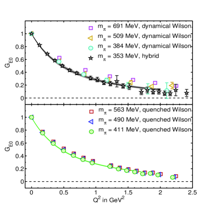
Figure 1: Comparison of the three different QCD lattice calculations for the $\Delta^{+}(1232)$ form factor $G_{E0}$. The upper curve shows a dipole fit to results using the mixed action. Results are also shown for two dynamical Wilson fermions. The lower curve is a dipole fit to results in the quenched approximation [16]. The error bands are calculated using a jackknife analysis of the fit parameters

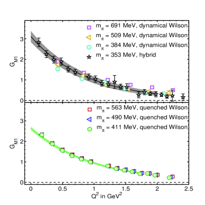
Figure 2: Comparison of the three different QCD lattice calculations for the $\Delta^{+}(1232)$ magnetic dipole form factors $G_{M1}$. The lines show the fits to an exponential form. The rest of the notation is the same as that in Fig. 1.

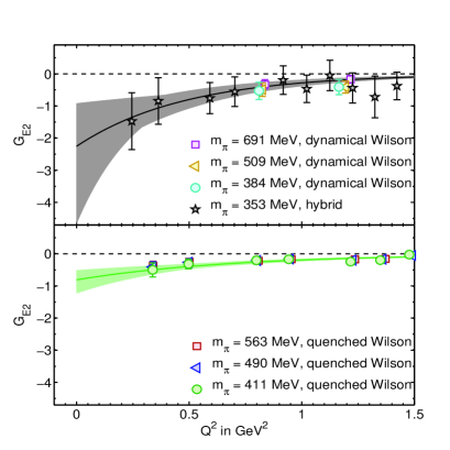
Figure 3: Comparison of the three different QCD lattice calculations for the $\Delta^{+}(1232)$ electric quadrupole form factors $G_{E2}$. The notation is the same as that in Fig. 1.

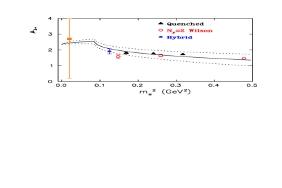
Figure 4: The magnetic dipole moment in nuclear magnetons. The value at the physical pion mass (filled square) is shown with statistical and systematic errors [2]. The solid and dashed curves show the results of ChEFT with the theoretical error estimate [17] .

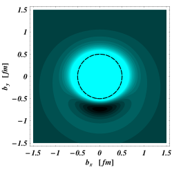
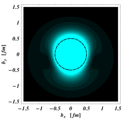
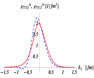
Figure 5: Quark transverse charge densities in a $\Delta^{+}(1232)$ which is polarized along the positive $x$-axis. Left panel : $\rho^{\Delta}_{T\,\frac{3}{2}}$. Middle panel : $\rho^{\Delta}_{T\,\frac{1}{2}}$. The light (dark) regions correspond with largest (smallest) values of the density. To better see the deformation, a circle of radius 0.5 fm is drawn for comparison. Right panel compares the density along the $y$-axis for $\rho^{\Delta}_{T\,\frac{3}{2}}$ (dashed curve) and $\rho^{\Delta}_{T\,\frac{1}{2}}$ (solid curve). For the $\Delta$ e.m. FFs, the quenched lattice QCD results are used.

The magnetic moment as function of $m_{\pi}^{2}$ is shown in Fig. 4, together with a comparison to a chiral effective field theory (ChEFT) result [17]. The ChEFT result has one free parameter (a low-energy constant) that has been fitted to lattice data, shown by the central line. We also estimate the uncertainty of the ChEFT expansion (expansion in pion mass) by the error band in Fig. 4. The uncertainty of the ChEFT calculation vanishes in the chiral limit because in this limit one simply has the value of the low-energy constant (LEC), which lies within the broad experimental error band $\mu_{\Delta^{+}}=2.7^{+1.0}_{-1.3}(stat.)\pm 1.5(syst.)\pm 3.0(theory)\mu_{N}$ [2]. In this work, we do not consider the uncertainty in the fit value of the LEC due to the lattice errors, as the calculations are still performed for pion masses where the $\Delta$ is stable (on the right side of the kink). A calculation for pion mass values where the $\Delta$ becomes unstable will be a challenge for future calculations. The $\Delta$ moments using an approach similar to ours are calculated only in the quenched approximation [18, 19, 20]. Our magnetic moment results agree with recent background field calculations using dynamical improved Wilson fermions [21]. The spatial length $L_{s}$ of our lattices satisfies $L_{s}m_{\pi}>4$ in all cases except at the lightest pion mass with $N_{F}=2$ Wilson fermions, for which $L_{s}m_{\pi}=3.6$. For that point, the magnetic moment falls slightly below the error band, consistent with the fact shown in Ref. [21] that finite volume effects decrease the magnetic moment.

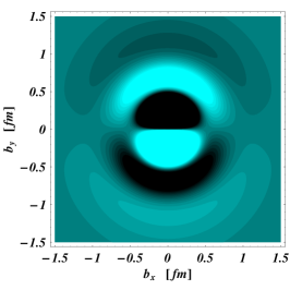
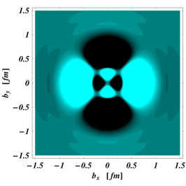
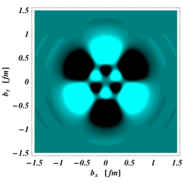
Figure 6: Different field patterns in the quark transverse charge density $\rho^{\Delta}_{T\,\frac{3}{2}}$ in a $\Delta^{+}(1232)$ which is polarized along the positive $x$-axis. Left panel : dipole field pattern; Middle panel : quadrupole field pattern; right panel : octupole field pattern. For the $\Delta$ e.m. FFs, the quenched lattice QCD results are used.

In Fig. 5, the transverse densities of Eqs. (3,4) are compared for a $\Delta^{+}$ which has a transverse spin. It is seen that the quark charge density in a $\Delta^{+}$ in a state of transverse spin projection $s_{\perp}=+3/2$ is elongated along the axis of the spin (prolate deformation) whereas in a state of transverse spin projection $s_{\perp}=+1/2$ it is elongated along the axis perpendicular to the spin. In Fig. 6 the dipole, quadrupole and octupole field patterns for the $\Delta$ transverse densities are clearly seen.

5 Conclusions

We have presented a study of the electromagnetic properties of the $\Delta(1232)$-resonance using lattice QCD. The lattice results for the $\Delta$ electromagnetic form factors have been shown here down to approximately 350 MeV for three cases: quenched QCD, two flavors of dynamical Wilson quarks, and three flavors of quarks described by a mixed action combining domain wall valence quarks and staggered sea quarks.

We have also worked out the formalism which allows to interpret these results in terms of the quark charge densities. More specifically, we have established the relation between the light-front helicity amplitudes and form factors for the case of electromagnetic interaction of a spin-3/2 particle, which allowed us to obtain the quark transverse charge densities of the $\Delta$ using lattice results for the form factors.

The light-front formalism allows for a consistent relation between the internal structure of the particle and its shape. Our lattice results show that the quark charge density in the $\Delta^{+}$ is elongated along the axis of the spin.

Acknowledgments: This work is supported in part by the Cyprus Research Promotion Foundation under contracts EPYAN/0506/08 and $\Delta$IE$\Theta$NH/$\Sigma$TOXO$\Sigma$/0308/07.

References

- [1] C. Alexandrou, G. Koutsou, J. W. Negele and A. Tsapalis, Phys. Rev. D 74 (2006) 034508; C. Alexandrou et al., Phys. Rev. D 69 (2004) 114506; C. Alexandrou, Ph. de Forcrand, H. Neff, J. W. Negele, W. Schroers and A. Tsapalis, Phys. Rev. Lett. 94 (2005) 021601; and references therein.
- [2] M. Kotulla et al., Phys. Rev. Lett. 89 (2002) 272001.
- [3] G. Lopez Castro and A. Mariano, Phys. Lett. B 517 (2001) 339.
- [4] W. M. Yao et al. [Particle Data Group], J. Phys. G 33 (2006) 1.
- [5] C. Alexandrou, C. N. Papanicolas and M. Vanderhaeghen, Rev. Mod. Phys., to appear.
- [6] C. Alexandrou, G. Koutsou, H. Neff, J. W. Negele, W. Schroers and A. Tsapalis, Phys. Rev. D 77, 085012 (2008) [arXiv:0710.4621 [hep-lat]].
- [7] C. Alexandrou et al., Phys. Rev. D 79, 014507 (2009) [arXiv:0810.3976 [hep-lat]].
- [8] C. Alexandrou et al., Nucl. Phys. A 825, 115 (2009) [arXiv:0901.3457 [hep-ph]].
- [9] C. E. Carlson and M. Vanderhaeghen, Eur. Phys. J. A 41, 1 (2009).
- [10] S. Nozawa and D. B. Leinweber, Phys. Rev. D 42 (1990) 3567.
- [11] C. Alexandrou, S. Gusken, F. Jegerlehner, K. Schilling and R. Sommer, Nucl. Phys. B 414 (1994) 815.
- [12] D. Dolgov et al. [LHPC collaboration], Phys. Rev. D 66 (2002) 034506.
- [13] R. G. Edwards et al. [LHPC Collaboration], Phys. Rev. Lett. 96, 052001 (2006) [arXiv:hep-lat/0510062].
- [14] Ph. Hagler et al. [LHPC Collaboration], Phys. Rev. D 77, 094502 (2008).
- [15] C. Aubin et al., Phys. Rev. D 70, 094505 (2004).
- [16] C. Alexandrou, T. Korzec, Th. Leontiou, J. W. Negele and A. Tsapalis, PoS(LAT2007), (2007),149, arXiv.0710.2744.
- [17] V. Pascalutsa and M.Vanderhaeghen, Phys. Rev. Lett. 94, (2005), 102003.
- [18] D. B. Leinweber, T. Draper and R. M. Woloshyn, Phys. Rev. D 46 (1992) 3067. [arXiv:hep-lat/9208025].
- [19] J.M. Zanotti, S. Boinepalli, D. B. Leinweber, A. G. Williams, A. G. and J. B. Zhang, Nucl. Phys. Proc. Suppl.,128 (2004), 233.
- [20] S. Boinepalli, J. N. Hedditch, B. G. Lasscock, D. B. Leinweber, A. G. Williams, J. M. Zanotti and J. B. Zhang, PoS LAT2006 (2006) 124.
- [21] C. Aubin, K. Orginos, V. Pascalutsa and M. Vanderhaeghen, arXiv:0809.1629 [hep-lat].
- [22] C. Aubin, K. Orginos, V. Pascalutsa and M. Vanderhaeghen, Phys. Rev. D 79, 051502 (R) (2009) [arXiv:0811.2440 [hep-lat]].