On the two-boson exchange corrections to
parity-violating elastic electron-proton scattering

Abstract

The details of the calculation of the two-boson exchange effects in the parity-violating elastic $ep$ scattering within a simple hadronic model, including both the nucleon and $\Delta(1232)$-resonance intermediate states, are presented. We examine the sensitivity of our results with respect to choice of form factors. We emphasize the importance to use correct relations relating $N\rightarrow\Delta$ and $\Delta\rightarrow N$ transition vertex functions. The $N\Delta$ Coulomb quadrupole transition is found to play important role at higher $Q^{2}\geq 3.0$ GeV². We also elucidate the relation between our results and the well-known result on the $\gamma ZE$ effect given by Marciano and Sirlin (MS). The effect of the nucleon contribution $\delta_{N}$ to parity-asymmetry $A_{PV}$, is found to be in general, larger than the corresponding $\Delta$ contribution $\delta_{\Delta}$ except at extreme forward angles. The corrections to the extracted values of the strange form factors $G^{s}_{E}+\beta G^{s}_{M}$ from the HAPPEX, A4, and G0 data are also presented. The total TBE corrections to the extracted values of $G^{s}_{E}+\beta G^{s}_{M}$ in recent experiments of HAPPEX G0, and A4 are, depending on kinematics, found to be small except in a few cases where they range from $-20.6\%$ to $48.3\%$.

I Introduction

One of the most intriguing questions in hadron structure is the possible existence of strangeness content in the proton since practically all constituent quark models employ only $u$ and $d$ quarks for light baryons. It was prompted by the EMC experiments EMC89 which indicate that the amount of spin carried by the strange quark pairs $s\bar{s}$ is comparable to that carried by the $u$ and $d$ quarks and polarized opposite to the nucleon spin. Similar conclusion was also drawn from elastic $\nu p$ scattering Ahrens87 and theoretical analysis of $\pi N$ sigma term Donoghue86 . A few other experiments have since been proposed Ellis01 , including the excess of $\phi$ production in $p\bar{p}$ annihilation Amsler98 , $\Lambda$ polarization in deep-inelastic neutrino scattering Ellis96 ; Nomad00 , and double polarizations in photo- and electroproduction of $\phi$ meson Titov97 scheduled at SPring8 for 2010 WCChang09 , and the parity-violating electron-proton scattering.

Parity-violating $ep$ scatterings was first suggested as a unique probe to extract proton strange form factors by Kaplan and Manohar Kaplan88 from measuring the parity-violating asymmetry $A_{PV}=(\sigma_{R}-\sigma_{L})/(\sigma_{R}+\sigma_{L})$ with polarized electrons, where $\sigma_{R(L)}$ is the cross section with a right-handed (left-handed) electron. The asymmetry arises from the interference of weak and electromagnetic amplitudes. Weak neutral current elastic scattering is mediated by the $Z$-boson exchange and measures form factors which are sensitive to a different linear combination of the three light quark distributions. When combined with proton and neutron electromagnetic form factors and with the use of charge symmetry, the strange electric and magnetic form factors, $G^{s}_{E}$ and $G^{s}_{M}$, can then be determined Kaplan88 . Since this is a rather clean technique to access the charge and magnetization distributions of the strange quark within nucleons, four experimental programs SAMPLE SAMPLE , HAPPEX HAPPEX , A4 A4 , and G0 G0 have been designed to measure this important quantity, which is small and ranges from 1 to 100 ppm. These experiments have been able to reach a precision of $\delta{A_{PV}}\sim 0.1$ ppm. Several global analyses have been performed Young06 ; Liu07 ; Pate08 and found that the electric and magnetic strange form factors are quite small with considerable error bars. Accordingly, greater effort to reduce theoretical uncertainty is needed in order to arrive at a more reliable interpretation of experiments.

Leading order radiative corrections to $A_{PV}$, including the box diagrams Fig. 1(d) and other diagrams, have been extensively studied Wheater82 ; Marciano83 ; Marciano84 ; Musolf90 and widely used in the global analyses in Young06 ; Liu07 ; Pate08 . Among those corrections, the interference between $\gamma Z$ exchange ($\gamma ZE$) of Fig. 1(d) with Fig. 1(a), was evaluated within the zero momentum transfer approximation, i.e., $Q^{2}=0$. The first calculation beyond the $Q^{2}=0$ approximation was done in afanasev05 where the contribution of the interference of the two-photon exchange ($2\gamma E$) process of Fig. 1(c) with diagram of Figs. 1(a) and 1(b) to $A_{PV}$, was evaluated in a partonic approach using GPDs. It was prompted by the fact that such a parton model calculation of the $2\gamma E$ effect Chen04 was arguably able to quantitatively resolve the discrepancy between the measurements of the proton electric to magnetic form factor ratio $R=\mu_{p}G_{E}/G_{M}$, where $\mu_{p}=2.79$, from Rosenbluth technique and polarization transfer technique at high momentum-transfer-squared $Q^{2}$ Jones00 . It was found afanasev05 that the $2\gamma E$ correction to $A_{PV}$ is both $Q^{2}$ and $\epsilon$ dependent, and can reach several percent in certain kinematics, becoming comparable in size with existing experimental measurements of strange-quark effects in the proton neutral weak current. However, the partonic calculations of afanasev05 ; Chen04 are reliable only for $Q^{2}$ large comparable to a typical hadronic scale, while all current experiments SAMPLE ; HAPPEX ; A4 ; G0 have been performed at lower $Q^{2}$ values.

The two-boson exchange (TBE) corrections to $A_{PV}$, namely, the contributions of the interference of the two-photon exchange ($2\gamma E$) process of Fig. 1(c) with diagram of Figs. 1(a) and 1(b) to $A_{PV}$, and that between the $\gamma Z$ exchange of Fig. 1(d) with Fig. 1(a), were investigated in a hadronic model first with only intermediate states restricted to elastic nucleon states in zhou07 ; tjon08 . This hadronic model was developed in Blunden03 to evaluate the $2\gamma E$ contribution to the ratio $R$. The advantage of such a hadronic approach Blunden03 is that it is applicable to low $Q^{2}$ region and the results obtained are in agreement with the partonic calculation of Chen04 . It is found zhou07 ; tjon08 that both the the $2\gamma E$ and $\gamma ZE$ corrections to $A_{PV}$ depends strongly on $Q^{2}$ and $\epsilon$, and can reach a few percent and are comparable in size with the current experimental measurements of strange quark effects in the proton weak neutral current and their combined effects on the extracted values of $G_{E}^{s}+\beta G_{M}^{s}$ can be as large as $-40\%$ in certain kinematics. It was further found tjon08 that the results show some sensitivity on whether a monopole or dipole form is assumed for the nucleon form factors.

Recently, the hadronic calculations on the TBE effects zhou07 ; tjon08 were extended to include $\Delta(1232)$ resonance in the intermediate states Nagata09 ; Tjon09 since $\Delta(1232)$ is known to play a dominant role in low-energy hadron physics pascal07 . Both calculations show that the interplay between the nucleon and $\Delta$ contributions depend strongly on the kinematics. However, there are discrepancies in the size of the total TBE corrections due to the use of different vertex relation relating the vertices of $\gamma N\rightarrow\Delta$ and $\gamma\Delta\rightarrow N$, the strength of the Coulomb quardrupole excitation of the $\Delta$, and the $\Delta$ form factors.

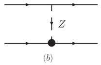
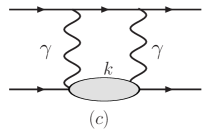
Figure 1: (a) One-photon exchange, (b) $Z$-boson exchange, (c) Two-photon exchange, and (d) $\gamma Z$-exchange diagrams for elastic ep scattering. Corresponding cross-box diagrams are implied.

In this paper, we give the details of our hadronic model calculations zhou07 ; Nagata09 of the $2\gamma E$ and $\gamma ZE$ corrections to $A_{PV}$ and present a more extensive results of our calculation. In particular we analyze in details the difference between our calculations and those of Ref. tjon08 ; Tjon09 . In addition, we demonstrate explicitly that our results do recover the results of Marciano84 in the limit of $Q^{2}=0$.

This article is organized as follows. The formalism for parity-violating electron-proton is given in Section II. The details of our calculation of the $\gamma ZE$ and $2\gamma E$ box diagrams in a simple hadronic model are presented in Section III. The numerical results of the above calculations and the impacts of our results on the extraction of the strange form factors and the weak charge of the proton are discussed in Section IV. In section V, we summarize our work.

II Parity-violating electron-proton elastic scattering

In this section we first briefly present the formulation of the parity-violating electron-proton elastic scattering within one-boson exchange (OBE) approximation and the corresponding procedure to extract the proton strange form factors. We then go beyond the OBE framework and discuss radiative corrections.

II.1 Parity-violating $ep$ scattering within one-boson-exchange approximation

The OBE diagrams of the elastic electron-proton scattering, $e(p_{1})+p(p_{2})\rightarrow e(p_{3})+p(p_{4})$, include one-photon exchange $(1\gamma E)$ and one-Z-boson exchange $(1ZE)$ diagrams, as shown in Fig. 1(a) and 1(b), respectively. At hadron level, the couplings of the photon and $Z$-boson with the proton are given as

$$\langle p^{\prime}|J^{Z}_{\mu}|p\rangle = \overline{u}(p^{\prime})\left[F^{Z,p}_{1}(q^{2})\gamma_{\mu}+F^{Z,p}_{2}(q^{2})\frac{i\sigma_{\mu\nu}}{2M_{N}}q^{\nu}+G^{Z}_{A}(q^{2})\gamma_{\mu}\gamma_{5}\right]u(p),$$

$$\langle p^{\prime}|J^{em}_{\mu}|p\rangle = \overline{u}(p^{\prime})\left[F^{\gamma,p}_{1}(q^{2})\gamma_{\mu}+F^{\gamma,p}_{2}(q^{2})\frac{i\sigma_{\mu\nu}}{2M_{N}}q^{\nu}\right]u(p),$$ (1)

where $M_{N}$ is the proton mass and $q=p^{\prime}-p$. $F^{\gamma/Z}_{1,2}$ and $G^{Z}_{A}$ are the proton electromagnetic/neutral weak current and axial form factors, respectively. The Sachs form factors are defined as

$$G_{E}^{\gamma/Z}=F_{1}^{\gamma/Z}-\tau F_{2}^{\gamma/Z},\,\,\,G_{M}^{\gamma/Z}=F_{1}^{\gamma/Z}+F_{2}^{\gamma/Z},$$ (2)

where $\tau=\frac{Q^{2}}{4M^{2}_{N}}$ with $Q^{2}=-q^{2}$. The OBE diagrams of Figs. 1(a) and 1(b) are given in terms of the matrix elements of the electromagnetic and neutral weak currents

$$M^{(a)} = -i\overline{u}(p_{3})(-ie\gamma^{\mu})u(p_{1})\frac{-i}{q^{2}+i\varepsilon}\overline{u}(p_{4})\Gamma^{\gamma}_{\mu}(p_{4},p_{2})u(p_{2}),$$

$$M^{(b)} = -i\overline{u}(p_{3})\left(\frac{ig\gamma^{\mu}}{4\cos\theta_{W}}\right)[(-1+4\sin^{2}\theta_{W})+\gamma_{5}]u(p_{1})\frac{-i}{q^{2}-M_{Z}^{2}+i\varepsilon}$$ (3)

$$\overline{u}(p_{4})\Gamma^{Z}_{\mu}(p_{4},p_{2})u(p_{2}),$$

where $\Gamma^{\gamma}_{\mu}(p^{\prime},p)=ie\langle N(p^{\prime})|J^{em}_{\mu}|N(p)\rangle$, $\Gamma^{Z}_{\mu}(p^{\prime},p)=(ig/4\cos\theta_{W})\langle N(p^{\prime})|J^{Z}_{\mu}|N(p)\rangle$. $g=e/\sin\theta_{W}$ is the weak coupling constant with $\theta_{W}$ the Weinberg weak mixing angle, and $M_{Z}$ the $Z$-boson mass. The parity asymmetry in OBE approximation arises from the interference of $M^{(a)}$ and $M^{(b)}$. Straightforward calculation, leads to the following expression of parity-asymmetry in OBE approximation in terms of the form factors defined in Eq. (1)

$$\begin{split}A_{PV}&=-\frac{G_{F}Q^{2}}{4\pi\alpha_{em}\sqrt{2}}\frac{A_{E}+A_{M}+A_{A}}{\bigl{[}\epsilon(G^{\gamma,p}_{E})^{2}+\tau(G^{\gamma,p}_{M})^{2}\bigr{]}},\\ A_{E}&=\epsilon G_{E}^{Z,p}G_{E}^{\gamma,p},~{}~{}A_{M}=\tau G_{M}^{Z,p}G_{M}^{\gamma,p},\\ A_{A}&=-(1-4\sin^{2}\theta_{W})\sqrt{\tau(1+\tau)(1-\epsilon^{2})}G_{A}^{Z}G_{M}^{\gamma,p},\end{split}$$ (4)

where $\epsilon\equiv[1+2(1+\tau)\tan^{2}\theta_{Lab}/2]^{-1}$ and $\theta_{Lab}$ the scattering angle of the electron in the laboratory frame. $G_{F}=\sqrt{2}g^{2}/8M_{W}^{2}=\pi\alpha_{em}/(\sqrt{2}M_{Z}^{2}\cos^{2}\theta_{W}\sin^{2}\theta_{W})=1.166\times 10^{-5}GeV^{-2}$ is the Fermi constant and $\alpha_{em}=e^{2}/4\pi$ the fine structure constant.

To extract the strange form factors from Eq. (4), one needs to make flavor decompositions of the form factors $G^{\gamma,p}_{E,M}$ and $G^{Z,p}_{E,M}$. In the standard model, the electromagnetic current and the neutral weak current are given as

$$J_{\mu}^{em}=\sum_{f=u,d,s}Q_{f}\bar{q}_{f}\gamma_{\mu}q_{f},\,\,\,J_{\mu}^{Z}=\sum_{f=u,d,s}\bar{q}_{f}\gamma_{\mu}(g^{f}_{V}+g^{f}_{A}\gamma_{5})q_{f},$$ (5)

where Musolf92 ,

$$g^{e}_{V} = -1+4\sin^{2}\theta_{W},\,\,g^{e}_{A}=+1,$$

$$g^{u}_{V} = 1-\frac{8}{3}\sin^{2}\theta_{W},\,\,g^{u}_{A}=-1,$$

$$g^{d}_{V} = -1+\frac{4}{3}\sin^{2}\theta_{W},\,\,g^{d}_{A}=+1,$$

$$g^{s}_{V} = -1+\frac{4}{3}\sin^{2}\theta_{W},\,\,g^{s}_{A}=-1.$$ (6)

From Eqs. (1,5,6), one obtains

$$G^{\gamma,p}_{E,M} = \frac{2}{3}G^{u/p}_{E,M}-\frac{1}{3}G^{d/p}_{E,M}-\frac{1}{3}G^{s/p}_{E,M},$$

$$G^{\gamma,n}_{E,M} = \frac{2}{3}G^{u/n}_{E,M}-\frac{1}{3}G^{d/n}_{E,M}-\frac{1}{3}G^{s/n}_{E,M},$$

$$G^{Z,p}_{E,M} = (1-\frac{8}{3}\sin^{2}\theta_{W})G^{u/p}_{E,M}+(-1+\frac{4}{3}\sin^{2}\theta_{W})G^{d/p}_{E,M}+(-1+\frac{4}{3}\sin^{2}\theta_{W})G^{s/p}_{E,M},$$ (7)

where $G^{q_{f}/p}_{E,M}$ are defined as follows

$$\langle p(p^{\prime})|\bar{q}_{f}\gamma_{\mu}q_{f}|p(p)\rangle=\overline{u}_{p}(p^{\prime})\left[F^{q_{f}/p}_{1}(q^{2})\gamma_{\mu}+F^{q_{f}/p}_{2}(q^{2})\frac{i\sigma_{\mu\nu}}{2M}q^{\nu}\right]u_{p}(p),$$ (8)

and

$$G_{E}^{q_{f}/p}=F_{1}^{q_{f}/p}-\tau F_{2}^{q_{f}/p},\,\,\,G_{M}^{q_{f}/p}=F_{1}^{q_{f}/p}+F_{2}^{q_{f}/p}.$$ (9)

If charge symmetry is assumed, i.e., the distribution of the $u$ quarks in the proton is the same as that of the $d$ quarks in the neutron, then one has $G^{u/p}_{E,M}=G^{d/n}_{E,M}$, $G^{d/p}_{E,M}=G^{u/n}_{E.M}$, and $G^{s/p}_{E,M}=G^{s/n}_{E,M}=G^{s}_{E,M}$ such that we can express the neutron electromagnetic form factors as

$$G^{\gamma,n}_{E,M}=\frac{2}{3}G^{d/p}_{E,M}-\frac{1}{3}G^{u/p}_{E,M}-\frac{1}{3}G^{s}_{E,M}.$$ (10)

Combining the first equation of Eq. (7) and Eq. (10) leads to the following two relations

$$G^{u/p}_{E,M}=2G^{\gamma,p}_{E,M}+G^{\gamma,n}_{E,M}+G^{s}_{E,M},\,\,\,G^{d/p}_{E,M}=G^{\gamma,p}_{E,M}+2G^{\gamma,n}_{E,M}+G^{s}_{E,M}.$$ (11)

Putting the above two relations of Eq. (11) back to the last relation in Eq. (7), the neutral weak form factors can be expressed in terms of the electromagnetic form factors of the proton and neutron, and the strange form factors

$$G_{E,M}^{Z,p}=(1-4\sin^{2}\theta_{W})G^{\gamma,p}_{E,M}-G^{\gamma,n}_{E,M}-G^{s}_{E,M}.$$ (12)

With Eq. (12), the parity asymmetry $A_{PV}$ of Eq. (4) can be rewritten as,

$$A_{PV}=A_{1}+A_{2}+A_{3},$$

$$A_{1}=-a\left[(1-4\sin^{2}\theta_{W})-\frac{\epsilon G^{\gamma,p}_{E}G^{\gamma,n}_{E}+\tau G^{\gamma,p}_{M}G^{\gamma,n}_{M}}{\epsilon(G^{\gamma,p}_{E})^{2}+\tau(G^{\gamma,p}_{M})^{2}}\right],$$

$$A_{2}=a\frac{\epsilon G^{\gamma,p}_{E}G^{s}_{E}+\tau G^{\gamma,p}_{M}G^{s}_{M}}{\epsilon(G^{\gamma,p}_{E})^{2}+\tau(G^{\gamma,p}_{M})^{2}},$$

$$A_{3}=a(1-4\sin^{2}\theta_{W})\frac{\epsilon^{\prime}G^{\gamma,p}_{M}G_{A}^{Z}}{\epsilon(G^{\gamma,p}_{E})^{2}+\tau(G^{\gamma,p}_{M})^{2}},$$ (13)

where $a=G_{F}Q^{2}/4\pi\alpha_{em}\sqrt{2}$ and $\epsilon^{\prime}=\sqrt{\tau(1+\tau)(1-\epsilon^{2})}$. The electromagnetic form factors $G^{\gamma,p}_{E,M}$ and $G^{\gamma,n}_{E,M}$ can be extracted from the elastic electron scattering from proton and deuteron (for the neutron), and the axial form factor $G^{Z}_{A}$ can be extracted from the pion photoproduction Bernard02 . Accordingly, one can extract $A_{2}$ from $A_{PV}$ to obtain the strange form factors $G^{s}_{E}+\beta G^{s}_{M}$ from $A_{2}$, with $\beta=\tau G^{\gamma,p}_{M}/\epsilon G^{\gamma,p}_{E}$, if radiative corrections can be neglected.

To take charge symmetry breaking effect into account, one may simply replace Eq. (12) with

$$G^{Z}_{E,M}=(1-4\sin^{2}\theta_{W})G^{\gamma,p}_{E,M}-G^{\gamma,n}_{E,M}-G^{s}_{E,M}-G^{CSB}_{E,M},$$ (14)

where $G^{CSB}_{E,M}=\frac{2}{3}\left(G^{d,p}_{E,M}-G^{u,n}_{E,M}\right)-\frac{1}{3}\left(G^{u,p}_{E,M}-G^{d,n}_{E,M}\right)$ and the extraction formula of Eq. (13) remains unchanged except $G^{s}_{E,M}$ be replaced by $\tilde{G}^{s}_{E,M}=G^{s}_{E,M}+G^{CSB}_{E,M}$. $G^{CSB}_{E,M}$ have been estimated in the constituent quark model Pollock95 ; Miller98 , light-cone meson-baryon model Ma97 , and chiral perturbation theory ($\chi$PT) Lewis99 with low-energy constants extracted from resonance saturation Kubis06 .

II.2 Radiative corrections to the parity-violating $ep$ scattering

Since the value of $A_{2}$ in Eq. (13) is just about a few percent of $A_{1}$, it is not possible to neglect the electroweak radiative corrections, which is of order ${\cal O}(\alpha_{em})$, to obtain accurate information of the strange form factors of the proton. This is the reason why high precision measurements and precise knowledge of the radiative corrections are required to obtain reliable extraction of the strange form factors from $ep$ scattering.

The complete ${\cal O}(\alpha_{em})$ radiative corrections to $A_{PV}$ derive from several different sources such as vertex corrections, self-energy insertions of the fermions and gauge bosons, $\gamma Z$ mixing, wave function renormalization, two-boson exchange, besides the inelastic bremsstrahlung. They have been extensively studied Wheater82 ; Marciano83 ; Marciano84 ; Musolf90 . The radiative corrections to $A_{PV}$ have been conventionally taken into account by expressing $A_{PV}$ in following form Musolf92

$$A_{PV}(\rho,\kappa)=A_{1}+A_{2}+A_{3},$$

$$A_{1}=-a\rho\left[(1-4\kappa\sin^{2}\theta_{W})-\frac{\epsilon G^{\gamma,p}_{E}G^{\gamma,n}_{E}+\tau G^{\gamma,p}_{M}G^{\gamma,n}_{M}}{\epsilon(G^{\gamma,p}_{E})^{2}+\tau(G^{\gamma,p}_{M})^{2}}\right],$$

$$A_{2}=a\rho\frac{\epsilon G^{\gamma,p}_{E}\tilde{G}^{s}_{E}+\tau G^{\gamma,p}_{M}\tilde{G}^{s}_{M}}{\epsilon(G^{\gamma,p}_{E})^{2}+\tau(G^{\gamma,p}_{M})^{2}},$$

$$A_{3}=a(1-4\sin^{2}\theta_{W})\frac{\epsilon^{\prime}G^{\gamma,p}_{M}G_{A}^{Z}}{\epsilon(G^{\gamma,p}_{E})^{2}+\tau(G^{\gamma,p}_{M})^{2}}.$$ (15)

When the parameters $\rho$ and $\kappa$ equal one, Eq. (15) reduces to Eq. (4), and one recovers the tree approximation. The linear combination of the strange form factors, $G^{s}_{E}+\beta G^{s}_{M}$, has been extracted from $A_{2}$ in Eq. (15). In this paper, we will restrict ourself to corrections arising from TBE.

III The amplitudes of two-boson exchange diagrams

In this section we evaluate the two-boson exchange diagrams in a simple hadronic model where the form factors are inserted as regulators and only the nucleon and $\Delta(1232)$ resonance intermediate states are included. We present the details of the calculation, including the explicit forms of the form factors and the values of parameters employed. As in Blunden03 ; zhou07 ; Nagata09 , we use package FeynCalc Feyncalc and LoopTools Looptools to do the analytical and numerical calculations, respectively.

III.1 The amplitudes of $2\gamma E$ and $\gamma Z$ exchange box diagrams

Choosing the Feynman gauge and neglecting the electron mass $m_{e}$ in the numerators, one can write down the amplitudes of box diagrams Fig. 1(c) and Fig. 1(d) with the nucleon intermediate states as

$$M^{(c,N)} = -i\int\frac{d^{4}k}{(2\pi)^{4}}\overline{u}(p_{3})(-ie\gamma^{\mu})\frac{i(p\!\!\!/_{1}+p\!\!\!/_{2}-k\!\!\!/)}{(p_{1}+p_{2}-k)^{2}-m_{e}^{2}+i\varepsilon}(-ie\gamma^{\nu})u(p_{1})$$

$$\times \frac{-i}{(p_{4}-k)^{2}-\lambda^{2}+i\varepsilon}\frac{-i}{(k-p_{2})^{2}-\lambda^{2}+i\varepsilon}\overline{u}(p_{4})\Gamma^{\gamma}_{\mu}(p_{4},k)\frac{i(k\!\!\!/+M_{N})}{k^{2}-M^{2}_{N}+i\varepsilon}\Gamma^{\gamma}_{\nu}(k,p_{2})u(p_{2}),$$

$$M^{(d,N)} = -i\int\frac{d^{4}k}{(2\pi)^{4}}\overline{u}(p_{3})(-ie\gamma^{\mu})\frac{i(p\!\!\!/_{1}+p\!\!\!/_{2}-k\!\!\!/)}{(p_{1}+p_{2}-k)^{2}-m_{e}^{2}+i\varepsilon}(i\frac{g\gamma^{\nu}}{4\cos\theta_{W}})$$ (16)

$$\times [(-1+4\sin^{2}\theta_{W}]+\gamma_{5})u(p_{1})\frac{-i}{(p_{4}-k)^{2}-\lambda^{2}+i\varepsilon}\frac{-i}{(k-p_{2})^{2}-M_{Z}^{2}+i\varepsilon}$$

$$\times \overline{u}(p_{4})\Gamma^{\gamma}_{\mu}(p_{4},k)\frac{i(k\!\!\!/+M_{N})}{k^{2}-M^{2}_{N}+i\varepsilon}\Gamma^{Z}_{\nu}(k,p_{2})u(p_{2}).$$

The amplitudes for the cross-box diagrams can be written down similarly. Because the amplitudes in Eq. (16) are infrared divergent, an infinitesimal photon mass $\lambda$ has been introduced in the photon propagators to regulate the IR divergence. As explained in zhou07 , in the soft photon limit, the box diagrams and their corresponding bremsstrahlung cross section give no correction to $A_{PV}$. To go beyond the soft photon approximation to estimate the corrections to $A_{PV}$, we calculate the full amplitudes of $M^{(c,N)}$ and $M^{(d,N)}$ and subtract $M^{(c,N)}_{soft}$ and $M^{(d,N)}_{soft}$ from their respective full amplitude. The interferences between the remaining box diagrams and the tree diagrams are then IR safe.

Similarly, amplitudes for the diagrams Fig. 1(c) and Fig. 1(d) with the $\Delta(1232)$ intermediate states can be written as follows

$$M^{(c,\Delta)} = -i\int\frac{d^{4}k}{(2\pi)^{4}}\overline{u}(p_{3})(-ie\gamma_{\mu})\frac{i(p\!\!\!/_{1}+p\!\!\!/_{2}-k\!\!\!/)}{(p_{1}+p_{2}-k)^{2}-m_{e}^{2}+i\varepsilon}\times(-ie\gamma_{\nu})u(p_{1})\frac{-i}{(p_{4}-k)^{2}+i\varepsilon}$$

$$\times \frac{-i}{(k-p_{2})^{2}+i\varepsilon}\overline{u}(p_{4})\Gamma^{\mu\alpha,\gamma}_{\Delta\rightarrow N}(k,p_{4}-k)\frac{-i(k\!\!\!/+M_{\Delta})P_{\alpha\beta}^{3/2}(k)}{k^{2}-M_{\Delta}^{2}+i\varepsilon}\Gamma^{\beta\nu,\gamma}_{N\rightarrow\Delta}(k,k-p_{2})u(p_{2}),$$

$$M^{(d,\Delta)} = -i\int\frac{d^{4}k}{(2\pi)^{4}}\overline{u}(p_{3})(-ie\gamma_{\mu})\frac{i(p\!\!\!/_{1}+p\!\!\!/_{2}-k\!\!\!/)}{(p_{1}+p_{2}-k)^{2}-m_{e}^{2}+i\varepsilon}(i\frac{g\gamma_{\nu}}{4\cos\theta_{W}})$$ (17)

$$\times ((-1+4\sin^{2}\theta_{W})+\gamma_{5})u(p_{1})\frac{-i}{(p_{4}-k)^{2}+i\varepsilon}\frac{-i}{(k-p_{2})^{2}-M_{Z}^{2}+i\varepsilon}$$

$$\times \overline{u}(p_{4})\Gamma^{\mu\alpha,\gamma}_{\Delta\rightarrow N}(k,p_{4}-k)\frac{-i(k\!\!\!/+M_{\Delta})P_{\alpha\beta}^{3/2}(k)}{k^{2}-M_{\Delta}^{2}+i\varepsilon}\Gamma^{\beta\nu,Z}_{N\rightarrow\Delta}(k,k-p_{2})u(p_{2}),$$

where

$$P_{\alpha\beta}^{3/2}(k)=g_{\alpha\beta}-\frac{\gamma_{\alpha}\gamma_{\beta}}{3}-\frac{(k\!\!\!/\gamma_{\alpha}k_{\beta}+k_{\alpha}\gamma_{\beta}k\!\!\!/)}{3k^{2}},$$ (18)

is the spin-3/2 projector. The amplitudes in Eq. (17) are IR finite because when the four-momentum of the photon approaches zero the $\gamma N\Delta$ vertices also approach zero. Therefore we do not need to put $\lambda$ in Eq. (17). The vertex functions $\Gamma^{\prime}s$ for $\Delta\rightarrow N$ are defined by

$$\overline{u}(p+q)\Gamma^{\mu\alpha,\gamma}_{\Delta\rightarrow N}(p,q)u^{\Delta}_{\alpha}(p)=-ie\langle N(p+q)|J^{\mu}_{em}|\Delta(p)\rangle,$$

$$\overline{u}(p+q)\Gamma^{\mu\alpha,Z}_{\Delta\rightarrow N}(p,q)u^{\Delta}_{\alpha}(p)=-ig\langle N(p+q)|J^{\mu}_{Z}|\Delta(p)\rangle,$$ (19)

and similarly vertex functions for $N\rightarrow\Delta$ are defined by

$$\overline{u}^{\Delta}_{\beta}(p)\Gamma^{\beta\nu,\gamma}_{N\rightarrow\Delta}(p,q)u(p-q)=-ie\langle\Delta(p)|J^{\nu}_{em}|N(p-q)\rangle,$$

$$\overline{u}^{\Delta}_{\beta}(p)\Gamma^{\beta\nu,Z}_{N\rightarrow\Delta}(p,q)u(p-q)=-ig\langle\Delta(p)|J^{\nu}_{Z}|N(p-q)\rangle.$$ (20)

Note that $q^{\prime}s$ in $\Gamma^{\mu\alpha,\gamma/Z}_{\Delta\rightarrow N}(p,q)$ and $\Gamma^{\beta\nu,\gamma/Z}_{N\rightarrow\Delta}(p,q)$ always correspond to the incoming momentum of the photon ($Z$ boson), a convention used in Blunden03 .

The relations between these vertex functions are

$$\Gamma^{\gamma}_{\Delta\rightarrow N}(p,q)=-\gamma_{0}[\Gamma^{\gamma}_{N\rightarrow\Delta}(p,-q)]^{\dagger}\gamma_{0},\,\,\,\Gamma^{Z}_{\Delta\rightarrow N}(p,q)=-\gamma_{0}[\Gamma^{Z}_{N\rightarrow\Delta}(p,-q)]^{\dagger}\gamma_{0}.$$ (21)

On the other hand, the following relations

$$\Gamma^{\gamma}_{\Delta\rightarrow N}(p,q)=\gamma_{0}[\Gamma^{\gamma}_{N\rightarrow\Delta}(p,q)]^{\dagger}\gamma_{0},\,\,\,\Gamma^{Z}_{\Delta\rightarrow N}(p,q)=\gamma_{0}[\Gamma^{Z}_{N\rightarrow\Delta}(p,q)]^{\dagger}\gamma_{0},$$ (22)

are used in Blunden03 ; Tjon09 . We consider Eq. (21) to be the correct one because it can be derived from the fact that both of the electromagnetic and neutral weak currents are Hermitian. The difference between Eq. (21) and Eq. (22) incurs discrepancies between the results obtained in Nagata09 and Tjon09 as will be discussed later.

III.2 Matrix elements of the electromagnetic and neutral weak currents
between nucleon and $\Delta$

Here we discuss the explicit forms of $\Gamma_{\Delta\rightarrow N}^{\gamma}$ and $\Gamma_{\Delta\rightarrow N}^{Z}$. The matrix elements of electromagnetic current between N and $\Delta$ is written as kondra05

$$\langle N(p^{\prime})|J^{em}_{\mu}|\Delta(p)\rangle = \frac{1}{M_{N}^{2}}\overline{u}(p^{\prime})[g_{1}F^{(1)}_{\Delta}(q^{2})(g^{\alpha}_{\mu}p\!\!\!/q\!\!\!/-p_{\mu}\gamma^{\alpha}q\!\!\!/-\gamma_{\mu}\gamma^{\alpha}p\cdot q+\gamma_{\mu}p\!\!\!/q^{\alpha})$$ (23)

$$+ g_{2}F^{(2)}_{\Delta}(q^{2})(p_{\mu}q^{\alpha}-p\cdot qg^{\alpha}_{\mu})$$

$$+ g_{3}F^{(3)}_{\Delta}(q^{2})/M_{N}(q^{2}(p_{\mu}\gamma^{\alpha}-g^{\alpha}_{\mu}p\!\!\!/)+q_{\mu}(q^{\alpha}p\!\!\!/-\gamma^{\alpha}p\cdot q))]\gamma_{5}T_{3}^{\dagger}u_{\alpha}(p),$$

where $q=p^{\prime}-p$ and $T_{3}$ is the third component of the $N\rightarrow\Delta$ isospin transition operator. $g_{i}$ are constants and $F^{(i)}_{\Delta}(q^{2}=0)=1$. One has the following relation between $G_{E,M,C}$, the transition form factors defined by Jones and Scadron Jones73 and $g_{1},\,g_{2},\,g_{3}$:

$$g_{1} = \frac{3}{2}\frac{M_{N}}{M_{\Delta}+M_{N}}(G_{M}(0)-G_{E}(0)),$$

$$g_{2} = \frac{3}{2}\frac{M_{N}(M_{\Delta}+3M_{N})}{M_{\Delta}^{2}-M_{N}^{2}}G_{E}(0)+\frac{3}{2}\frac{M_{N}}{M_{\Delta}+M_{N}}G_{M}(0),$$

$$g_{3} = -\frac{3}{2}\frac{M_{N}^{2}}{M_{\Delta}(M_{\Delta}+M_{N})}\left(-\frac{M_{\Delta}+M_{N}}{M_{\Delta}-M_{N}}G_{C}(0)+\frac{4M_{\Delta}^{2}}{(M_{\Delta}-M_{N})^{2}}G_{E}(0)\right)$$ (24)

We take $G_{M}(0)=3.02$ Tiator01 . $G_{E}(0)$ and $G_{C}(0)$ can be inferred from the relations $G_{E}(0)=-G_{M}(0)R_{EM}$ and $G_{C}(0)=-[4M_{\Delta}^{2}/(M_{\Delta}^{2}-M_{N}^{2})]G_{M}(0)R_{SM}$ with the experimentally determined values of $R_{EM}=-2.5\%$ Beck00 ; DMT and $R_{SM}=-4.0\%$ MAID07 . We thus have $G_{E}(0)=0.0755$ and $G_{C}(0)=1.1496$ and correspondingly, $g_{1}=1.91$, $g_{2}=2.63$, and $g_{3}=1.57$. Note that the normalization used in Eq. (23) to define the couplings constants $g_{i}^{\prime}s$ differs from that of kondra05 ; Tjon09 where they used $M_{\Delta}$ instead of $M_{N}$ everywhere in Eq. (23). With this normalization difference taken into account, the corresponding values of $g_{i}^{\prime}s$ used in Tjon09 would be $g_{1}=1.82$ and $g_{2}=2.81$, with $g_{3}$ varied from -0.44 to 1.28. We note that, however, since all the current experimental data for $R_{SM}$ extracted from experiments at low $Q^{2}$’s as small as $Q^{2}=0.060$ GeV² Stave06 remain negative, we will not consider the possibility of a negative value of $g_{3}$. The difference between the values of $g_{3}$ used in our calculation and Tjon09 leads to considerable differences in some of the results between these two calculations, if the vertex relation of Eq. (21) is employed, as will be discusses in the next section.

The neutral weak current can be decomposed into isovector and isoscalar parts:

$$J^{Z}_{\mu} = \alpha_{V}V^{3}_{\mu}+\beta_{A}A^{3}_{\mu}+\rm{isoscalar}\,\,\rm{terms},$$

$$J^{em}_{\mu} = V^{3}_{\mu}+\rm{isoscalar}\,\,\rm{terms},$$ (25)

where the superscript ”3” refers to the third component in isospin space, $\alpha_{V}=(1-2\sin^{2}\theta_{W})/(2\cos\theta_{W})$ and $\beta_{A}=-1/(2\cos\theta_{W})$. The isoscalar part does not contribute to $N\rightarrow\Delta$ transition. The $Zp\Delta^{+}$ vertex contains both the vector and the axial-vector components. The vector part takes the form

$$\langle p(p^{\prime})|J^{Z}_{\mu,V}|\Delta^{+}(p)\rangle = \frac{1}{M_{N}^{2}}\overline{u}(p^{\prime})[\tilde{g}_{1}F^{(1)}_{\Delta}(q^{2})(g^{\alpha}_{\mu}p\!\!\!/q\!\!\!/-p_{\mu}\gamma^{\alpha}q\!\!\!/-\gamma_{\mu}\gamma^{\alpha}p\cdot q+\gamma_{\mu}p\!\!\!/q^{\alpha})$$ (26)

$$+ \tilde{g}_{2}F^{(2)}_{\Delta}(q^{2})(p_{\mu}q^{\alpha}-p\cdot qg^{\alpha}_{\mu})$$

$$+ \tilde{g}_{3}F^{(3)}_{\Delta}(q^{2})/M_{N}(q^{2}(p_{\mu}\gamma^{\alpha}-g^{\alpha}_{\mu}p\!\!\!/)+q_{\mu}(q^{\alpha}p\!\!\!/-\gamma^{\alpha}p\cdot q))]\gamma_{5}u_{\alpha}(p),$$

where $\tilde{g}_{i}^{\prime}s$ and $g_{i}^{\prime}s$ are related by $\tilde{g}_{i}=\sqrt{2/3}\,\alpha_{V}g_{i}.$ Note that the factor $\sqrt{\frac{2}{3}}$ comes from isospin transition operator $T_{3}^{\dagger}$. Thus we have $\tilde{g}_{1}=0.47$, $\tilde{g}_{2}=0.658$ and $\tilde{g}_{3}=0.40$.

The axial-vector component of the $Zp\Delta^{+}$ vertex is given as Nagata09

$$\langle p(p^{\prime})|J^{Z}_{\mu,A}|\Delta^{+}(p)\rangle = \frac{1}{M_{N}^{2}}\overline{u}(p^{\prime})[h_{1}H^{(1)}_{\Delta}(q^{2})(g^{\alpha}_{\mu}(p\cdot q)-p_{\mu}q^{\alpha})$$ (27)

$$+ h_{2}H^{(2)}_{\Delta}(q^{2})/M_{N}^{2}(q^{\alpha}q_{\mu}p\!\!\!/q\!\!\!/-(p\cdot q)\gamma^{\alpha}q_{\mu}q\!\!\!/)+h_{3}H^{(3)}_{\Delta}(q^{2})((p\cdot q)\gamma^{\alpha}\gamma_{\mu}-p\!\!\!/\gamma_{\mu}q^{\alpha})$$

$$+ h_{4}H^{(4)}_{\Delta}(q^{2})(g^{\alpha}_{\mu}p^{2}-p_{\mu}\gamma^{\alpha}p\!\!\!/)]u^{\Delta}_{\alpha}(p),$$

where $F^{(i)}_{\Delta}$ in Eq. (26) and $H^{(i)}_{\Delta}$ in Eq. (27) are the vector and axial-vector form factors, respectively. In the present investigation, we will assume that, for simplicity, some of them separately takes a common form for different couplings, i.e., $F^{(i)}_{\Delta}=F_{\Delta}(Q^{2})$ and $H^{(i)}_{\Delta}=H_{\Delta}(Q^{2})$. In addition, both $F_{\Delta}$ and $H_{\Delta}$ are normalized to one at $Q^{2}=0$.

Only the coupling constants $h_{i}^{\prime}s$ remain to be determined. They can be obtained from the data of $\nu N\rightarrow\mu\Delta$. Many experimental papers on neutrino induced $\Delta$ production adopt the notation of Llewellyn-Smith smith where the $N\Delta$ transition induced by the weak charged axial-current is written as

$$\langle\Delta^{++}(p^{\prime})|J^{W,A}_{\mu}|p(p)\rangle = \overline{u}_{\alpha}(p^{\prime})[\frac{C^{A}_{3}(Q^{2})}{M_{N}}(q\!\!\!/g^{\alpha}_{\mu}-q^{\alpha}\gamma_{\mu})+\frac{C^{A}_{4}(Q^{2})}{M^{2}_{N}}((p^{\prime}\cdot q)g^{\alpha}_{\mu}-q^{\alpha}p^{\prime}_{\mu})$$ (28)

$$+ C^{A}_{5}(Q^{2})g^{\alpha}_{\mu}+\frac{C^{A}_{6}(Q^{2})}{M_{N}^{2}}p^{\alpha}q_{\mu}]u(p).$$

The form factors in Eq. (27) can be related to the form factors defined in Eq. (28) by performing a rotation in isospace and assuming the nucleon and $\Delta$ are both on-shell. The resulting relations are

$$h_{1}= -\frac{\beta C^{A}_{4}(0)}{\sqrt{3}}-\frac{2M_{N}}{M_{\Delta}}\,\frac{\beta C^{A}_{3}(0)}{\sqrt{3}},$$ (29)

$$h_{3}= \frac{M_{N}}{M_{\Delta}}\cdot\frac{\beta C^{A}_{3}(0)}{\sqrt{3}},\,h_{2}=-\frac{M_{N}^{2}}{M_{\Delta}(M_{\Delta}-M_{N})}\,\frac{\beta C^{A}_{6}(0)}{\sqrt{3}},$$

$$h_{4}= \frac{M_{N}^{2}}{M_{\Delta}^{2}}\frac{\beta C^{A}_{5}(0)}{\sqrt{3}}+\frac{M_{N}(M_{\Delta}-M_{N})}{M_{\Delta}^{2}}\,\frac{\beta C^{A}_{3}(0)}{\sqrt{3}}.$$

According to Adler68 and Schreiner73 , $C_{3}^{A}=0$ and hence $h_{3}=0$. If we follow the weak pion production data of Kitagaki90 and extrapolate the experimental result to $Q^{2}=0$ Hemmert95 , then we find $C^{A}_{4}(0)=-0.8,\,\,\,C^{A}_{5}(0)=2.4,$ to obtain $h_{1}=-0.263,\,\,h_{4}=-0.458$. The parameter $h_{2}$ cannot be determined from the weak pion production. According to partial conservation of axial current (PCAC), one has the following relation

$$C_{6}^{A}(Q^{2})\approx\frac{M^{2}_{N}}{m_{\pi}^{2}+Q^{2}}C^{A}_{5}(Q^{2}),$$ (30)

where $m_{\pi}$ is the pion mass. Hence one obtains $C^{A}_{6}(0)\approx\frac{M^{2}_{N}}{m_{\pi}^{2}}C^{A}_{5}(0)\approx 107.7$ and the corresponding value for $h_{2}$ would be about $-360.91$. Even with such a large value, we find its effect is tiny ($\leq 10^{-16}$) and therefore we simply set $h_{2}=0$.

Note that the vertices $\gamma N\Delta$ and $ZN\Delta$ in Eqs. (23, 26, 27) all satisfy the constraints:

$$p_{\alpha}\Gamma^{\mu\alpha}_{\Delta\rightarrow N}(p,q^{\prime})=p_{\beta}\Gamma^{\beta\nu}_{N\rightarrow\Delta}(p,q^{\prime})=0,$$ (31)

for any $q^{\prime}$, to eliminate the coupling of the unphysical spin-1/2 component of Ratria-Schwinger spinor Pascal99 . The expressions in Eqs. (26, 27) have been written in many different ways smith ; Nath ; Hemmert95 but only those given here satisfy the above constraints.

In Tjon09 , different forms of the axial form factors are employed. They obtain the matrix elements of $J^{Z}_{\mu,A}$ by simply removing $\gamma_{5}$ from Eq. (26) and write

$$\Gamma^{\mu\alpha,Z}_{\Delta\rightarrow N} = \frac{i}{2M_{\Delta}^{2}}[g_{1}^{A}(Q^{2})[g^{\mu\alpha}p\!\!\!/q\!\!\!/-p^{\mu}\gamma^{\alpha}q\!\!\!/-\gamma^{\mu}\gamma^{\alpha}(p\cdot q)+\gamma^{\mu}q^{\alpha}p\!\!\!/]$$ (32)

$$+ g_{2}^{A}(Q^{2})[p^{\mu}q^{\alpha}-g^{\mu\alpha}(p\cdot q)]$$

$$+ \frac{g_{3}^{A}(Q^{2})}{M_{\Delta}}[q^{2}(p^{\mu}\gamma^{\alpha}-g^{\mu\alpha}p\!\!\!/)-q^{\mu}(q^{\alpha}p\!\!\!/-\gamma^{\alpha}(p\cdot q))]].$$

It leads to only three form factors instead of four in Eq. (27). The form factor $g_{3}^{A}(Q^{2})$ of Eq. (32) is required to have a pole at $Q^{2}=0$. However, form factors defined in Eq. (27) are not required to have such poles, and in our opinion, a more appropriate choice.

III.3 Nucleon and $N\rightarrow\Delta$ form factors

So far we have not specified the explicit forms of the nucleon and $N\rightarrow\Delta$ form factors. In this article we adopt the following two sets of the form factors. The set A is parametrized as follows:

$$G^{\gamma,p}_{E} = G^{\gamma,p}_{M}/\mu_{p}=G^{Z,p}_{E}/x=G^{Z,p}_{M}/y=\frac{\Lambda^{4}_{1}}{(Q^{2}+\Lambda^{2}_{1})^{2}},$$

$$G^{Z,p}_{A}/z = \frac{\Lambda^{4}_{2}}{(Q^{2}+\Lambda^{2}_{2})^{2}},$$ (33)

where $x=G^{Z,p}_{E}(Q^{2}=0)$, $y=G^{Z,p}_{M}(Q^{2}=0)$ and $z=G^{Z}_{A}(Q^{2}=0)$. We take $\Lambda_{1}=0.84\,$ GeV and $\Lambda_{2}=1.0\,$ GeV from the usual dipole form $G^{\gamma,p}_{E}=1/(1+Q^{2}/0.71)^{2}$, and $G^{Z}_{A}=G^{Z}_{A}(0)/(1+Q^{2})^{2}$ HAPPEX ; Beise , with $Q$ given in unit of $GeV$, i.e., $c=1$, a convention to be used hereafter. We determine $x,y,z$ from relations Beise , $G^{Z,p}_{E,M}=\rho(1-4\kappa\sin^{2}\theta_{W})G^{\gamma,p}_{E,M}-\rho G^{s}_{E,M}-\rho G^{\gamma,n}_{E,M}$ and $G^{Z}_{A}=-(1+R_{A}^{T=1})G_{A}+\sqrt{3}R_{A}^{T=0}G_{A}^{8}+\Delta s$ at $Q^{2}=0$ point. The quantities $G_{A}^{8}$ and $\Delta s$ refer to the $SU(3)$ isoscalar octet form factor and the strange quark contribution to the nucleon spin, respectively. The $\rho,\kappa$ and $R_{A}^{T=1}$ and $R_{A}^{T=0}$ are due to radiative corrections. They lead to $x=0.076\pm 0.00264$, $y=2.08\pm 0.00813-G_{M}^{s}(0),z=-0.95^{+0.37}_{-0.36}+\Delta s(0)$. We fix $x=0.076$ and vary the values of $y,z,\Lambda_{1},$ and $\Lambda_{2}$ to check the sensitivity of the results on the parameters and find little changes.

The forms of the $\gamma N\Delta$ and $ZN\Delta$ are taken to be

$$F_{\Delta}(Q^{2})=\frac{\Lambda_{1}^{4}}{(Q^{2}+\Lambda^{2}_{1})^{2}},\,\,\,H_{\Delta}(Q^{2})=\frac{\Lambda^{4}_{2}}{(Q^{2}+{\Lambda}^{2}_{2})^{2}}.$$ (34)

Variations of these cutoffs are found not to affect the results significantly as well.

The form factors set A given in Eqs. (33) and (34) do not describe well the existing data at large $Q^{2}$. For example, the ratio of the proton electric to magnetic form factors $R=\mu_{p}G_{E}/G_{M}$ has been found to deviate from one at large $Q^{2}$ Jones00 , while the form factors of Eq. (33) gives $R=1$. Similarly, the $N\rightarrow\Delta$ transition form factors have been measured and found to drop faster than $Q^{-4}$ at high $Q^{2}$. More specifically, perturbative QCD predicts that at high $Q^{2}$, the Jones-Scadron form factors scale as follows Carlson86 ,

$$G_{M}(Q^{2})\sim Q^{-4},\,\,G_{E}(Q^{2})\sim Q^{-4},\,\,G_{C}(Q^{2})\sim Q^{-6},$$ (35)

such that both $R_{EM}$ and $R_{SM}$ should approach some constants as $Q^{2}\rightarrow\infty$. The $N\rightarrow\Delta$ transition form factors given in Eq. (34) clearly do not have the correct asymptotic behavior at high $Q^{2}$. We try to take these into account by adding extra factors to both $G^{\gamma,p}_{E}$ and $F^{(i)}_{\Delta}$ given in Eqs. (33) and (34). This leads to the following more realistic form factors set B, with $F^{(1,2)}_{\Delta}(Q^{2})=F_{\Delta}(Q^{2})$,

$$G^{\gamma,p}_{M}/\mu_{p} = \left(\frac{\Lambda_{1}^{2}}{Q^{2}+\Lambda_{1}^{2}}\right)^{2},\,G^{\gamma,p}_{E}=\left(\frac{\Lambda_{1}^{2}}{Q^{2}+\Lambda_{1}^{2}}\right)^{2}\frac{\Lambda_{3}^{2}}{Q^{2}+\Lambda_{3}^{2}},\,G^{Z,p}_{A}=\frac{\Lambda_{1}^{2}}{Q^{2}+\Lambda_{1}^{2}},$$

$$F_{\Delta}(Q^{2}) = \left(\frac{\Lambda_{1}^{2}}{Q^{2}+\Lambda_{1}^{2}}\right)^{2}\frac{\Lambda_{4}^{2}}{Q^{2}+\Lambda_{4}^{2}},\,\,\,F^{(3)}_{\Delta}=F_{\Delta}(Q^{2})\left(\frac{\Lambda_{5}^{2}}{Q^{2}+\Lambda_{5}^{2}}\right),\,$$

$$H_{\Delta} = \left(\frac{\Lambda_{1}^{2}}{Q^{2}+\Lambda_{1}^{2}}\right)^{2}.$$ (36)

Fitting the data of Jones00 ; Sato07 gives $\Lambda_{3}=2.0$ GeV, $\Lambda_{4}=\sqrt{2}$ GeV and $\Lambda_{5}=0.5$ GeV. Note that when one evaluates the effect from the box diagrams with $\Delta$ intermediate states, one still needs to specify the choice of the nucleon form factors because one still receives contribution from the interference between $1\gamma E$ and TBE box diagrams. Therefore each form factors set includes both of nucleon and $N\rightarrow\Delta$ form factors. We will discuss the sensitivity of the results with respect to the use of these two different sets of the form factors in Sec IV.

IV Results and Discussions

In this section, we present the results of the corrections of $2\gamma E$ and $\gamma ZE$ to $A_{PV}$ in the simple hadronic model described in the previous section. The sensitivity with respect to different choices of parameters and form factors will be analyzed in details. The influence of the TBE effects on the extracted values of the strange form factors $G^{s}_{E}+\beta G^{s}_{M}$ is discussed at the end.

IV.1 TBE Effects on $A_{PV}$

As in zhou07 ; Nagata09 , we characterize the $2\gamma E$ and $\gamma ZE$ corrections to $A_{PV}$ by $\delta$ defined as

$$A_{PV}(1\gamma+Z+2\gamma+\gamma Z)=A_{PV}(1\gamma+Z)(1+\delta_{N}+\delta_{\Delta}),$$ (37)

where $A_{PV}(1\gamma+Z)$ denotes the parity-violating asymmetry arising from the interference between $1\gamma$ and $Z$-boson exchange, i.e., Figs. 1(a) and 1(b) while $A_{PV}(1\gamma+Z+2\gamma+\gamma Z)$ includes the effects of $2\gamma E$ and $\gamma ZE$ with the nucleon and $\Delta(1232)$ intermediate states. $\delta_{N(\Delta)}$ represents the contribution from the diagrams with the nucleon ($\Delta$-resonance) intermediate states, respectively.

IV.1.1 The TBE corrections from the nucleon intermediate states

Figure 2: $2\gamma E$ and $\gamma ZE$ corrections to $A_{PV}$ with nucleon intermediate states, as functions of $\epsilon$ from 0.1 to 0.99 at $Q^{2}=0.03,\,0.1,\,1.0,$ and $5.0\,$ GeV², respectively. Dotted and dashed lines denote corrections coming only from interferences of $1\gamma\times 2\gamma$, and $Z\times 2\gamma$ . The solid lines represent contributions of $\gamma\times\gamma Z$. The lines in red and black correspond to the results using the form factors set A and B, respectively.

We first present the results of $\delta_{N}$ as function of $\epsilon$, the contributions of TBE diagrams with the nucleon intermediate states, in Fig. 2. The effects of the interferences between $1\gamma E$ and $2\gamma E$ ($1\gamma\times 2\gamma$), and those between $1ZE$ and $2\gamma E$ ($Z\times 2\gamma$) are represented by the dotted and dashed lines, respectively, at four different $Q^{2}$ values, $Q^{2}$=0.03,  0.1,  1.0,  5.0 GeV². The interferences between $1\gamma E$ and $\gamma ZE$ are given by the solid lines. The lines in red correspond to the results obtained with form factors set A while the black lines are associated with form factors set B, as specified in Eqs. (33-36) in the previous section. We see little difference between red and black curves in Fig. 2, as both form factors sets A and B are of dipole or higher order forms. On the contrary, in Fig. 3 one finds that at $Q^{2}=5.0$ GeV² the results using the monopole form factors, with cut-offs adjusted accordingly, are much smaller than those obtained with sets A and B, as pointed out in tjon08 .

In Fig. 2, we see that both $2\gamma E$ and $\gamma ZE$ effects strongly depend on $Q^{2}$ and $\epsilon$. The magnitude of each contribution has its maximum at $\epsilon=0$ and decrease to zero when $\epsilon$ increases. One also sees that $1\gamma\times 2\gamma$ contribution always cancels the $Z\times 2\gamma$ contribution and hence their sums are always small compared with the size of each contribution, a feature also present in the partonic calculation of Ref. afanasev05 . Another interesting fact is that the magnitude of $\delta_{N}(1\gamma\times 2\gamma)$ is always larger than $\delta_{N}(Z\times 2\gamma)$. For the $1\gamma\times\gamma Z$ contribution, it decreases as $Q^{2}$ increases and dominates over $\delta_{N}(2\gamma E)$ at the backward directions when $Q^{2}\leq 0.1\,$ GeV², but reduces to about the same size as the total $2\gamma E$ contribution at higher $Q^{2}$.

Figure 3: $1\gamma\times 2\gamma$ and $Z\times 2\gamma$ corrections to $A_{PV}$ with nucleon intermediate states, as functions of $\epsilon$ from 0.1 to 0.99 at $Q^{2}=5.0\,$ GeV². Dotted lines denote the results obtained with monopole type form factors. Dashed and solid lines correspond to results obtained with form factors sets A and B, respectively.

IV.1.2 The TBE corrections from the $\Delta$(1232) intermediate states

Figure 4: $2\gamma E$ and $\gamma ZE$ corrections to $A_{PV}$, with $\Delta$(1232) intermediate states as functions of $\epsilon$ at $Q^{2}=0.03,\,0.1,\,1.0,$ and $5.0\,$ GeV². Dotted and dashed lines denote corrections coming only from the interference $1\gamma\times 2\gamma$, and $Z\times 2\gamma$, respectively. The solid lines represent the contribution of $\gamma\times\gamma Z$. The lines in red and black correspond to results obtained with form factors set A and B, respectively.

We continue to present our result of $\delta_{\Delta}$ which arises from the TBE diagrams with the $\Delta(1232)$ intermediate states. In Fig. 4, we show the $2\gamma E$ and $\gamma ZE$ corrections to $A_{PV}$ by plotting $\delta_{\Delta}\,\,vs.\,\,\epsilon$ for both form factors sets A and B. Again, the red and the black lines correspond to results obtained with form factors set A and B, respectively. One immediately notices that they are very close to each other when $Q^{2}\leq 0.1$ GeV². However, difference begins to develop when $Q^{2}$ reaches 1.0 GeV² at forward angles ($\epsilon\geq$ 0.8). As $Q^{2}$ increases further, the difference between red and black lines becomes more pronounced even at small $\epsilon$ and at $Q^{2}=5.0$ GeV², the discrepancy reaches more that $100\%$ in some cases. The fact that $\delta_{\Delta}$ is more sensitive than $\delta_{N}$ to the details of the form factors indicates that the TBE diagrams with the $\Delta$ intermediate states are more strongly dependent on the higher loop momentum than the diagrams with the nucleon intermediate states.

One further observes that the contributions of $1\gamma\times 2\gamma$ and $Z\times 2\gamma$ are negligible for $Q^{2}\leq$ 0.1 GeV². As $Q^{2}$ increases, the magnitudes of both contributions increase and become comparable in size with $\delta_{\Delta}(\gamma\times\gamma Z)$ as $Q^{2}$ reaches 5.0 GeV². The cancelation between $1\gamma\times 2\gamma$ and $Z\times 2\gamma$ contributions is also seen in Fig. 4 with the magnitude of $1\gamma\times 2\gamma$ contribution larger than that of $Z\times 2\gamma$ as in the $\delta_{N}$ case.

The $\gamma\times\gamma Z$ contribution exhibits more complicated $Q^{2}$ and $\epsilon$ dependence. At lower $Q^{2}\leq 0.1GeV^{2}$, it remains small until $\epsilon$ reaches between $0.6\sim 0.8$. Then it increases rapidly before dropping drastically when $\epsilon$ becomes very close to one. For $Q^{2}$ in the region of $0.1\sim 1.0$ GeV², $\gamma ZE$ contribution is flat and almost zero until $\epsilon$ increases past 0.8 and becomes small and negative at forward angles. The behavior changes when $Q^{2}$ grows larger than 1.0 GeV², as it decreases monotonically with increasing $\epsilon$, crosses zero at $\epsilon\sim 0.7$, and drops rapidly as $\epsilon$ reaches 0.9.

To sum up, we see that at lower $Q^{2}\leq$ 0.1 GeV², $\gamma ZE$ contribution dominates. When $Q^{2}$ reaches 5 GeV², $1\gamma\times 2\gamma$ effect becomes dominant at backward angles and brings the full $\delta_{\Delta}$ into negative. However, at forward angles the $1\gamma\times 2\gamma$ contribution cancels the sum of $1Z\times 2\gamma$ and $\gamma\times\gamma Z$ and the total $\delta_{\Delta}$ becomes negligible.

Figure 5: The short-dashed and solid lines correspond to the results using vertex function relations Eq. (22) and Eq. (21), respectively.

Hereafter, we will restrict ourself to results of $\delta_{\Delta}$ obtained with form factors set B.

$\delta_{\Delta}$ has been calculated independently by Nagata09 and Tjon09 . The results are different because of the following two reasons. The first is that different relations between vertex functions of $\Gamma_{N\rightarrow\Delta}$ and $\Gamma_{\Delta\rightarrow N}$ are employed. The other arises from employing different values of $g_{3}$, the Coulomb quadrupole excitation strength of $N\rightarrow\Delta$.

In general, there are four diagrams associated with the $\gamma ZE$ diagram depicted in Fig. 1(d), two by interchanging the order of the exchanged $\gamma$ and $Z$ lines and two others from the associated cross-box diagrams. For simplicity, let’s just consider only the two box diagrams without cross. We denote the amplitude of the diagram with $\gamma$ exchanged first by $M_{\gamma Z}$ and the other with $Z$ exchanged first by $M_{Z\gamma}$, both with the $\Delta$ in the intermediate states and only the vector $ZN\Delta$ coupling. We may then write

$$\delta_{\gamma Z} = \sum_{i,j=1}^{3}\tilde{g_{j}}g_{i}C_{ji},$$

$$\delta_{Z\gamma} = \sum_{i,j=1}^{3}g_{i}\tilde{g_{j}}C_{ji}^{\prime}.$$ (38)

Our numerical results for the magnitudes of $C_{ji}$ agree Tjon09a with those obtained in Tjon09 . However, with the use of the vertex relation of Eq. (22), one would obtain

$$C_{13}=-C^{\prime}_{13},\,\,C_{23}=-C^{\prime}_{23},\,\,C_{31}=-C^{\prime}_{31},\,\,C_{32}=-C^{\prime}_{32},$$ (39)

where the subscripts 1, 2, and 3 correspond to M1, E2, and C2 couplings, respectively, and $C_{ij}=C^{\prime}_{ij}$ for the rest. On the other hand, there would be no minus signs in Eq. (39) if the vertex relation of Eq. (21) is used. Consequently, after summing up $\delta_{\gamma Z}$ and $\delta_{Z\gamma}$, the crossing-couplings of C2 with M1 and E2 terms give no contribution in the calculation of Tjon09 , while in Nagata09 no cancelation between $\delta_{\gamma Z}$ and $\delta_{Z\gamma}$ occurs at all. Similar situation also takes place with the amplitudes where the vertex $ZN\Delta$ is of axial-vector coupling. The resulting discrepancy in the predictions for $\delta_{\Delta}$ are shown in Figs. 5 and 6.

In the upper two figures of Fig. 5, we show the difference arising from using vertex function relations of Eqs. (21) and (22) for two fixed values of $Q^{2}=0.1$ and 3.0 GeV². The solid and short-dashed lines correspond to the results using Eq. (21) and Eq. (22). At low $Q^{2}$, discrepancy is small. However at higher $Q^{2}$ the difference between two results is significant at the forward angles. In the lower two figures of Fig. 5, on the other hand, $\epsilon$ is fixed at 0.5 and 0.99, respectively, while $Q^{2}$ is varied. We see large difference develop at large $Q^{2}$ in both cases. Furthermore, when $\epsilon$ is fixed at 0.99, the solid line goes downward but the dashed line goes upward, and when $Q^{2}$ reaches 6.0 GeV² the solid line goes down to about -0.04 but the dashed line is almost zero.

Figure 6: The dotted and solid lines denote results obtained with $g_{3}=0$, and $g_{3}=1.57$, respectively.

In Fig. 6, the dotted and solid lines denote the results obtained with $g_{3}=0$ and $g_{3}=1.57$ as used in Nagata09 , respectively. The difference at low $Q^{2}$ cases is very small but becomes significant as $Q^{2}$ reaches 3.0 GeV², especially at the forward angles. It underscores the important role played by the Coulomb quadrupole transition in the evaluation of the box diagrams with $\Delta$ intermediate states at high $Q^{2}$ and large $\epsilon$. In Tjon09 , $g_{3}$ (in our convention), was varied from $-0.44$ to $1.28$ and the effects of varying $g_{3}$ are found to be small. It is because the use of the vertex relation of Eq. (22) leads to cancelations in the cross couplings between C2, and M1 and E2 such that the effects of $g_{3}$ is reduced. Another reason is that only cases up to $Q^{2}\sim 1.0$ GeV² are explored.

IV.1.3 Total effects: sum of $\delta_{N}$ and $\delta_{\Delta}$

Here we compare the behavior of $\delta_{N}$ and $\delta_{\Delta}$ and present their sum. We see from Fig. 7 that both of them are sensitive to $Q^{2}$ and $\epsilon$. At $Q^{2}=0.03$ GeV², $\delta_{N}$ is dominant over $\delta_{\Delta}$ in the range $0\leq\epsilon\leq 0.6$ because $\delta_{\Delta}$ is negligible there. As $\epsilon$ further increases, $\delta_{\Delta}$ increases rapidly at $\epsilon=0.6$ before dropping at extremely forward angles. These behaviors are in sharp contrast with $\delta_{N}$ which simply decreases as $\epsilon$ increases. The qualitative features of the curves at $Q^{2}=0.1$ GeV² remain the same with the one at $Q^{2}=0.03$ GeV².

When $Q^{2}$ increases to 1.0 GeV², one sees that $\delta_{\Delta}$ is very small and flat while $\delta_{N}$ decreases monotonously with respect to $\epsilon$. As $Q^{2}$ increases up to 5 GeV², $\delta_{\Delta}$ becomes negative at backward angles but becomes positive as $\epsilon$ increases. On the contrary $\delta_{N}$ is always positive. We conclude that at small $\epsilon$, $\delta_{N}$ is dominant but $\delta_{\Delta}$ becomes important as $\epsilon$ grows.

Another way to compare $\delta_{N}$ with $\delta_{\Delta}$ is to see the evolution of the $\delta^{\prime}s$ w.r.t. $Q^{2}$ at fixed $\epsilon$ as depicted in Fig. 8 for $\epsilon=0.5$ and $\epsilon=0.8$. The notation is the same as in Fig. 7. We clearly see that for at $\epsilon=0.5$, $\delta_{\Delta}$ is small and of opposite sign to $\delta_{N}$, while at larger value of $\epsilon=0.8$, is always comparable with $\delta_{N}$ and becomes dominant at large value of $Q^{2}$.

Since $\delta_{N}$ is substantially larger that $\delta_{\Delta}$ in the region $\epsilon\leq 0.8$, the total effect $\delta=\delta_{N}+\delta_{\Delta}$ is very close to $\delta_{N}$. They differ only after $\epsilon$ grows larger than $\sim 0.8$.

More quantitatively, at $Q^{2}=0.1$ GeV², the full correction, i.e., the combined effect of $\delta_{N}$ and $\delta_{\Delta}$, reaches about 1.75% at backward angle 135^∘ (SAMPLE), about 1.68% at forward angle 35^∘ (A4) and about -0.4% at very forward angle 6^∘ (HAPPEX). On the other hand, when $Q^{2}$ grows to 1.0 GeV², the full correction starts from around $1.4\%$ at backward angles and decreases to become less than $-0.4\%$ at extreme forward angles.

Figure 7: Two-boson exchange corrections with nucleon (dotted) and $\Delta$ (dashed) intermediate states to $A_{PV}$, as functions of $\epsilon$ from 0.1 to 0.9 at $Q^{2}=0.03,\,\,0.1,\,\,1.0,$ and $5.0$ GeV², respectively. The solid lines denote their sums $\delta=\delta_{N}+\delta_{\Delta}$.

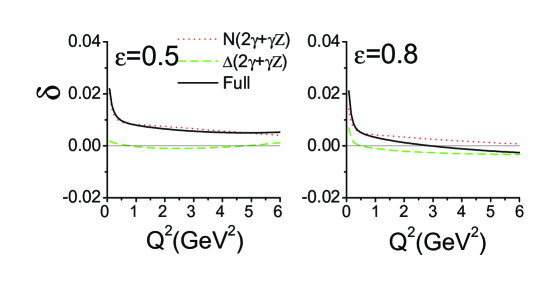
Figure 8: Two-boson exchange corrections with an intermediate nucleon (dotted) and $\Delta$ (dashed) states to $A_{PV}$, as functions of $Q^{2}$ from 0.1 to 6 GeV² at $\epsilon=0.5$ and 0.8, respectively. The solid lines denote their sums $\delta=\delta_{N}+\delta_{\Delta}$.

IV.1.4 Comparison with Marciano-Sirlin approximation

Here we elucidate the relation between our results with those obtained within MS approximation Marciano84 . Upon close inspection, the method of MS actually contains three approximations. The first one is to assume the momentum transfer $Q=p_{1}-p_{3}=p_{4}-p_{2}=0$. Furthermore in the MS approximation the electron mass is neglected and $E_{lab}$ is taken to be zero. This is the second approximation used by MS. Lastly, they take away the Coulomb interactions because it was argued that its effect has been included in the wave function of the bounded electron since they were concerned with the atomic systems.

Moreover, the MS approximation includes no contribution from the resonance intermediate states. Hence we shall compare our results for $\delta_{N}(1\gamma\times\gamma Z)\equiv\bar{\delta}_{N}$ with values obtained in the MS approximation. Since we have already seen that the results do depend somewhat on the form factors, we will employ the same form factors used in Marciano84 in order to make the comparison more exact.

We first define some quantities to facilitate the comparison. In the MS approximation, the parity asymmetry due to the $\gamma Z$ diagrams is given by,

$$A_{PV}^{MS,\gamma Z}(Q^{2},E_{lab})=\frac{2Re[M^{(a)\dagger}M^{PV,MS}_{\gamma Z}]}{|M^{(a)}|^{2}},$$ (40)

where $M^{(a)}$ is the $1\gamma E$ of Eq. (3) and $M^{PV,MS}_{\gamma Z}$ the parity-violating part of the $\gamma ZE$ amplitude evaluated within the MS approximation scheme. The $Q^{2}$ and $E_{lab}$ dependence of Eq. (40) arises entirely from $M^{(a)}$ because $M_{\gamma Z}^{PV,MS}$ is taken at $Q^{2}=0$ and $E_{lab}=0$.

We further introduce the following quantity,

$$\delta_{MS}(Q^{2},E_{lab})=\frac{A_{PV}^{MS,\gamma Z}(Q^{2},E_{lab})}{A_{PV}^{OBE}(Q^{2},E_{Lab})}=\frac{2Re[M^{(a)\dagger}M^{PV,MS}_{\gamma Z}]/|M^{(a)}|^{2}}{2Re[M^{(a)\dagger}M^{(b)}]/|M^{(a)}|^{2}}=\frac{Re[M^{(a)\dagger}M^{PV,MS}_{\gamma Z}]}{Re[M^{(a)\dagger}M^{(b)}]}.$$ (41)

On the other hand, the $\bar{\delta}_{N}$ we obtain is given as

$$\bar{\delta}_{N}(Q^{2},E_{lab})=\frac{A_{PV}^{\gamma Z}(Q^{2},E_{lab})}{A_{PV}^{OBE}(Q^{2},E_{Lab})}=\frac{2Re[M^{(a)\dagger}M^{PV,HM}_{\gamma Z}]/|M^{(a)}|^{2}}{2Re[M^{(a)\dagger}M^{(b)}]/|M^{(a)}|^{2}}=\frac{Re[M^{(a)\dagger}M^{PV,HM}_{\gamma Z}]}{Re[M^{(a)\dagger}M^{(b)}]},$$ (42)

where $M^{(b)}$ is the $1ZE$ amplitude of Eq. (3) and $M^{PV,HM}_{\gamma Z}$ the parity-violating part of the $\gamma ZE$ amplitude evaluated in our hadronic model with only the nucleon intermediate states included, with both dependent on $Q^{2}$ and $E_{lab}$. The relation between $\bar{\delta}_{N}$ and $\delta_{MS}$ is most transparent when $Q^{2}=0,E_{lab}=0$ because $M_{\gamma Z}^{PV,MS}$ is evaluated at this point. In this limit, $\delta_{MS}$ is given Marciano84 as,

$$\Delta_{MS}\equiv\delta_{MS}(Q^{2}=0,E_{lab}=0)=\rho_{\gamma Z}-\frac{4\kappa_{\gamma Z}\sin^{2}\theta_{W}}{1-4\sin^{2}\theta_{W}}=\frac{5\alpha_{em}}{2\pi}\left[K+\frac{4}{5}\xi_{B}\right],$$ (43)

where $\rho_{\gamma Z}$ and $\kappa_{\gamma Z}$ are

$$\rho_{\gamma Z} = -\frac{2\alpha_{em}}{\pi}(1-4\sin^{2}\theta_{W})\left[K+\frac{4}{5}\xi_{B}\right],$$

$$\kappa_{\gamma Z} = -\frac{\alpha_{em}}{2\pi\sin^{2}\theta_{W}}\left(\frac{9}{4}-4\sin^{2}\theta_{W}\right)(1-4\sin^{2}\theta_{W})\left[K+\frac{4}{5}\xi_{B}\right].$$ (44)

Here $K$ is the asymptotic contribution obtained by carrying out the short-distance expansion in a free-field theory. Its value is 8.58 if the onset scale is set to be 1 GeV. On the other hand, $\frac{4}{5}\xi_{B}$ corresponds to the the long-distance contribution of the $\gamma Z$ box diagram estimated in the Born approximation. Its value has been estimated to be 2.04.

Hence one obtains $\Delta_{MS}(low-k)=1.18\%$ and $\Delta_{MS}(high-k)=4.98\%$. It was argued in Tjon09 that the hadronic calculation as done here should correspond to the so-called soft part because the form factors used in the hadronic calculation function serves as a regulator and the contribution from the higher loop momentum are suppressed. Accordingly, our result for $\bar{\delta}_{N}(Q^{2},E_{lab})$ should reproduce $\Delta_{MS}(low-k)=1.18\%$ in the proper MS limit as we discuss next.

In Fig. 9 we present our results for $\bar{\delta}_{N}(Q^{2},E_{lab})$ by setting $Q^{2}=0$ with varying $E_{lab}$. The full results and the Coulomb contribution are denoted by the solid and short-dashed lines, respectively. The difference between the solid and short-dashed curves, represented by the long-dashed line, would correspond to the low-k contribution, to be compared with results of Marciano84 . One sees that the long-dashed line, when $E_{lab}$ goes to zero, does approach 1.18%, a value given in the MS approximation if only low-k contribution is kept.

Figure 9: Comparison between our result for $\bar{\delta}_{N}\equiv\delta_{N}(1\gamma\times\gamma Z)$ of Eq. (42) at $Q^{2}=0$ with $\Delta_{MS}$ of Eq. (43)as obtained within MS approximation. The dashed line denotes the contribution corresponding to the low-k part of the MS approximation with finite $E_{lab}$. The Coulomb part is represented by the dotted line and the total contribution is denoted as the solid line.

In other words, our calculation restores the value given by MS approximation if we follow their scheme. On the other hand, it is easy to see that the Coulomb interaction contribution is larger as compared with the non-Coulomb part. Furthermore the non-Coulomb contribution decreases more rapidly as $E_{lab}$ increases. Note that the calculation in this section is carried out at $Q^{2}=0$. We see that the $\gamma ZE$ contributions is sensitive to $E_{lab}$ and it is necessary to go beyond the MS approximation.

IV.2 Extraction of the strange form factors

Here we first examine the effects of the $2\gamma E$ and $\gamma ZE$ on the values of strange form factors extracted from HAPPEX HAPPEX , A4 A4 , and G0 experiments where data have been taken at forward angles. In SAMPLE experiment, measurements of both elastic $ep$ and electron-deuteron ($eD$) scatterings are combined to extract $G_{M}^{s}$. However, due to the fact that there is no reliable way to estimate the TPE and $\gamma ZE$ contributions to elastic $eD$ scattering, we do not know how to reanalyze SAMPLE data. Naively, one may attempt to apply the simple hadronic model here to the deuteron case. But as the deuteron is a loosely bound system, treating deuteron in a similar manner as proton is questionable.

IV.2.1 The formulation of the extraction of the strange form factors

All the existing analyses Young06 ; Liu07 ; Pate08 extract strange from factors from Eq. (15) where the electroweak radiative corrections are included in the parameters of $\rho$ and $\kappa$ in the expression. The latest PDG values PDG2008 for $\rho$ and $\kappa$ are $\rho=0.9876$ and $\kappa=1.0026$. They deviate from one because higher-order contributions like vertex corrections, corrections to the propagators, and TBE effects are taken into account. Since we have explicitly calculated the effect of TBE effects in this study, we should replace the contribution of TBE to the above-mentioned $\rho$ and $\kappa$ as estimated by MS, with our results to avoid double counting. Namely, one should then subtract $\Delta\rho=\rho_{\gamma Z}$ and $\Delta\kappa=\kappa_{\gamma Z}$ from $\rho$ and $\kappa$ and use $\rho^{\prime}=\rho-\Delta\rho$ and $\kappa^{\prime}=\kappa-\Delta\kappa$ in Eq. (15) instead.

As explained earlier, $\rho_{\gamma Z}$ and $\kappa_{\gamma Z}$ in Eq. (44) actually consist of two contributions, namely, the high-k and low-k parts and our results correspond to the low-k part only. We should then only take away the soft loop momentum contribution, which is associated with the $\xi_{B}$ term, and define $\Delta\rho,\Delta\kappa$ as follows:

$$\Delta\rho = -\frac{2\alpha_{em}}{\pi}(1-4\sin^{2}\theta_{W})\cdot\frac{4}{5}\xi_{B}=-0.73\times 10^{-3}$$

$$\Delta\kappa = -\frac{\alpha_{em}}{2\pi\sin^{2}\theta_{W}}\left(\frac{9}{4}-4\sin^{2}\theta_{W}\right)(1-4\sin^{2}\theta_{W})\cdot\frac{4}{5}\xi_{B}=-1.03\times 10^{-3}.$$ (45)

Consequently, we set the experimental parity asymmetry $A_{PV}^{(Exp)}$ as follows:

$$A_{PV}^{(Exp)} \equiv A_{PV}(1\gamma+Z+2\gamma+\gamma Z),$$ (46)

$$= A_{PV}(\rho^{\prime},\kappa^{\prime})(1+\delta).$$

With the value we obtain for $\delta$, we can determine $A_{PV}(\rho^{\prime},\kappa^{\prime})$ and extract the strange form factors from the resultant $A_{2}$ of Eq. (13).

Furthermore, we introduce

$$\overline{G}_{E}^{s}+\beta\overline{G}_{M}^{s}=(G_{E}^{s}+\beta G_{M}^{s})(1+\delta_{G}),$$ (47)

to quantify the effects of the $2\gamma E$ and $\gamma ZE$ to the extracted values of $G^{s}_{E}+\beta G^{s}_{M}$, where $G_{E}^{s}+\beta G_{M}^{s}$ and $\overline{G}_{E}^{s}+\beta\overline{G}_{M}^{s}$ are extracted from $A_{PV}(\rho,\kappa)$ and $A_{PV}(\rho^{\prime},\kappa^{\prime})$, respectively. From

$$G^{s}_{E}+\beta G^{s}_{M} = \frac{\epsilon(G^{\gamma,p}_{E})^{2}+\tau(G^{\gamma,p}_{M})^{2}}{a\rho\epsilon G^{\gamma,p}_{E}}\left[A^{Exp}_{PV}-A_{1}(\rho,\kappa)-A_{3}\right],$$

$$\overline{G}^{s}_{E}+\beta\overline{G}^{s}_{M} = \frac{\epsilon(G^{\gamma,p}_{E})^{2}+\tau(G^{\gamma,p}_{M})^{2}}{a\rho^{\prime}\epsilon G^{\gamma,p}_{E}}\left[\frac{A^{Exp}_{PV}}{1+\delta}-A_{1}(\rho^{\prime},\kappa^{\prime})-A_{3}\right],$$ (48)

we get,

$$\delta_{G} = \frac{A^{Exp}_{PV}(\frac{\Delta\rho}{\rho}-\delta)+4a\rho\sin^{2}\theta_{W}\Delta\kappa-\frac{\Delta\rho}{\rho}A_{3}}{A^{Exp}_{PV}-A_{0}}$$ (49)

$$= \left(\frac{-A^{Exp}_{PV}}{A^{Exp}_{PV}-A_{0}}\right)\delta+\left(\frac{4a\rho\sin^{2}\theta_{W}}{A^{Exp}_{PV}-A_{0}}\right)\Delta\kappa+\left(\frac{A^{Exp}_{PV}-A_{3}}{A^{Exp}_{PV}-A_{0}}\right)\frac{\Delta\rho}{\rho}$$

$$= \eta_{1}\delta+\eta_{2}\Delta\kappa+\eta_{3}\frac{\Delta\rho}{\rho},$$

where $A_{0}=A_{1}(\rho,\kappa)+A_{3}$. Note that the values of $\eta_{1}$, $\eta_{2}$, and $\eta_{3}$ all depend on the values of the inputs of the nucleon form factors such as $G^{\gamma,p}_{E,M}$, $G^{\gamma,n}_{E,M}$ and $G^{Z}_{A}$. As a result, the value of $\delta_{G}$ also depends on those inputs.

We further define $\delta_{0}$, the corresponding value of $\delta$ as would be obtained in Marciano84 within $Q\equiv 0$ approximation scheme such that $\delta_{G}=0$ if $\delta=\delta_{0}$. In other words, difference between $\delta$ as we obtain and $\delta_{0}$, represents the possible $Q^{2}$-dependence neglected in the estimation of Marciano83 , such that $\delta_{G}$ vanishes when $\delta=\delta_{0}$. Explicitly the value of $\delta_{0}$ is given by

$$\delta_{0}=-\frac{\eta_{2}}{\eta_{1}}\Delta\kappa-\frac{\eta_{3}}{\eta_{1}}\frac{\Delta\rho}{\rho}.$$ (50)

Obviously the value of $\delta_{0}$ depends on the inputs of the proton and neutron electromagnetic form factors as well.

IV.2.2 Extraction of the strange form factors at HAPPEX, A4, and G0 experiments

At forward angles, $A_{3}$ in Eq. (15) is negligible because both $\epsilon^{\prime}=\sqrt{\tau(1-\tau)(1-\epsilon^{2})}\ll 1$ and $1-4\sin^{2}\theta_{W}\ll 1$. It offers some advantages that the strange form factors can then be determined more accurately. This is why many experiments, like HAPPEX, A4, and G0 are carried out at very forward angles. In Table 1, we present our results for $\delta_{N},\,\delta_{\Delta},\,$ their sum $\delta$, besides $\delta_{0}$ and $\delta_{G}$, for HAPPEX HAPPEX , A4 A4 , and G0 G0 experiments. They are obtained with the use of form factors set B. We also list the values of $G_{s}\equiv G_{E}^{s}+\beta G_{M}^{s}$. For the G0 experiments, only measurements of $A_{PV}$ are given in G0 and the corresponding values of $G_{s}$ listed in Table 1 are extracted by us with the use of the nucleon electromagnetic factors parametrized in Alberico09 . The resultant change in the values of $G_{s}$ after TBE effects are properly taken into account, i.e., $\Delta G_{s}\equiv(\bar{G}_{E}^{s}+\beta\bar{G}_{M}^{s})-(G_{E}^{s}+\beta G_{M}^{s})$, are given in the last column of Table 1.

Exp	$Q^{2}(GeV^{2})$	$\epsilon$	$\delta_{N}(\%)$	$\delta_{\Delta}(\%)$	$\delta(\%)$	$\delta_{0}(\%)$	$\delta_{G}(\%)$	$G_{s}(10^{-2})$	$\Delta G_{s}(10^{-2})$
HAPPEX	0.477	0.974	0.18	-0.27	-0.09	0.20	-2.54	1.4	-0.04
HAPPEX	0.109	0.994	0.21	-0.80	-0.58	0.51	-20.63	0.7	-0.14
G0	0.122	0.9930	0.21	-0.72	-0.51	0.61	-3.63	3.9	-0.14
G0	0.128	0.9926	0.21	-0.70	-0.49	1.05	-1.28	9.2	-0.12
G0	0.136	0.9921	0.21	-0.67	-0.44	0.81	-1.60	7.7	-0.12
G0	0.144	0.9916	0.20	-0.64	-0.41	0.38	14.14	-1.1	-0.16
G0	0.153	0.9911	0.20	-0.61	-0.39	0.51	-3.50	3.8	-0.13
G0	0.164	0.9904	0.20	-0.58	-0.36	0.41	-9.18	1.5	-0.14
G0	0.177	0.9896	0.20	-0.55	-0.32	0.31	6.19	-2.3	-0.14
G0	0.192	0.9886	0.19	-0.52	-0.29	0.35	-16.05	0.8	-0.12
G0	0.210	0.9875	0.19	-0.48	-0.29	0.30	48.25	-0.3	-0.14
G0	0.232	0.9860	0.19	-0.44	-0.25	0.30	-20.25	0.6	-0.12
G0	0.262	0.9840	0.19	-0.40	-0.21	0.35	-2.26	4.6	-0.10
G0	0.299	0.9814	0.19	-0.36	-0.17	0.26	-8.68	1.2	-0.10
G0	0.344	0.9783	0.19	-0.32	-0.13	0.28	-1.99	4.4	-0.09
G0	0.411	0.9735	0.19	-0.27	-0.08	0.27	-1.18	6.4	-0.08
G0	0.511	0.9657	0.20	-0.23	-0.03	0.19	-2.10	2.8	-0.06
G0	0.628	0.9580	0.21	-0.20	0.01	0.20	-0.71	6.8	-0.05
G0	0.786	0.9413	0.22	-0.18	0.04	0.15	-0.81	3.9	-0.03
G0	0.997	0.9197	0.25	-0.18	0.07	0.15	-0.32	7.6	-0.02
A4	0.108	0.83	1.07	0.53	1.60	0.61	2.00	7.1	0.14
A4	0.23	0.83	0.66	0.14	0.80	0.29	2.85	3.9	0.11

Table 1: The values of $\delta_{N},\delta_{\Delta}$, and their sum $\delta$ for the HAPPEX HAPPEX , G0 G0 , and A4 A4 data. We give the values of $\delta_{0}$, $\delta_{G}$, $G_{s}$, and $\Delta G_{s}$ obtained with $g_{3}=1.57$, for those data points.

All experimental data included in Table 1 were obtained in the near forward directions with $\epsilon\geq 0.8$. More specifically, the HAPPEX and G0 data were taken at extremely forward angles with $\epsilon\geq 0.92$. It is seen from Table 1 that in this region there is a cancelation between $\delta_{N}$ and $\delta_{\Delta}$ as they are of opposite sign. The magnitude of $\delta_{\Delta}$ is always larger than $\delta_{N}$ at lower $Q^{2}\leq 0.7$ GeV². When $Q^{2}$ increases past 0.7 GeV², $\delta_{N}$ overtakes $\delta_{\Delta}$ and the sum $\delta$ becomes positive. On the other hand, in the kinematical regions of A4 data, both $\delta_{N}$ and $\delta_{\Delta}$ are positive such that the sum $\delta$ is also positive.

Furthermore, one notices that $\delta_{0}$ is in general larger than $\delta_{N}$. It implies that MS approximation overestimates the TBE contribution, besides neglecting the strong $Q^{2}$ dependence.

The values of $\delta_{G}$ presented in Table 1 are considerably smaller than what we reported in Nagata09 . It can be understood from the following reasons. First, the values of $\delta^{\prime}s$ listed are already different from before since they are obtained with different nucleon and $N\rightarrow\Delta$ form factors. Previously in zhou07 ; Nagata09 , the nucleon form factors used are of monopole type while the $N\Delta$ transition form factors are taken to be of dipole form. In addition, $\rho_{\gamma Z}$ and $\kappa_{\gamma Z}$ obtained here are now used to replace only the soft part contribution evaluated by MS, i.e., the $\Delta\rho$ and $\Delta\kappa$ of Eq. (45), as emphasized in Tjon09 . For example, for the HAPPEX data at $Q^{2}=0.109$ GeV² and $\epsilon=0.994$, the value of $\delta_{G}$ in Nagata09 is given as $-75.23\%$. However if we use the value of $\delta=-0.58\%$ in Table 1 instead of the previous $\delta=-1.19\%$, then $\delta_{G}$ is reduced to $-60.52\%$. If we further use the value of $\kappa_{\gamma Z}=-1.03\times 10^{-3}$ identified as the hadronic contribution in Marciano84 instead of the value of $-5.33\times 10^{-3}$, then value of $\delta_{G}$ becomes $-14.99\%$. Lastly, using the value of $\Delta\rho=-0.73\times 10^{-3}$ given in Eq. (45), instead of the value of $-3.72\times 10^{-3}$, produces small change and leads to the final value of $\delta_{G}=-20.63\%$ as given in Table I.

In general, the values of $\delta_{G}$ are smaller than 10% and are mostly negative with the exception of backward data of A4. For HAPPEX data at $Q^{2}=0.109$ GeV² and G0 data at $Q^{2}=0.144,\,0.192,\,0.210$ and 0.232 GeV², the magnitudes of $\delta_{G}$ are large and range between $-20.95\%$ to $63.73\%$. The magnitudes of $\delta_{G}$ seem to behave irregularly. However if one computes the $\Delta G_{s}\equiv(\bar{G}_{E}^{s}+\beta\bar{G}_{M}^{s})-(G_{E}^{s}+\beta G_{M}^{s})$, the values of $\Delta{G}_{s}$ are relatively stable with typical size of $-(0.1\sim 0.2)\times 10^{-2}$. It is because those with large values of $\delta_{G}$ have small values of $G_{s}$.

Lastly, to illustrate the sensitivity of the corrections to the extracted strange form factors, with respect to the possible experimental uncertainties in the extracted value of $R_{SM}$ and the resulting Coulomb quardrupole excitation strength of the $\Delta(1232)$, we give in Table II our results for $\delta_{\Delta},\,\delta\,\ \delta_{0}$, and $\delta_{G}$, obtained with $g_{3}=0$ for some of the HAPPEX, A4, and G0 data. Comparison between Tables I and II shows that the variations in the final corrections to the extracted values of the strange form factors, when $g_{3}$ changes from 0 to 1.57, amount to about 20$\%$.

Exp	$Q^{2}(GeV^{2})$	$\epsilon$	$\delta_{\Delta}(\%)$	$\delta(\%)$	$\delta_{G}(\%)$	$\Delta G_{s}(10^{-2})$
HAPPEX	0.477	0.974	-0.30	-0.13	-2.81	-0.04
HAPPEX	0.109	0.994	-0.94	-0.73	-23.36	-0.16
G0	0.128	0.9926	-0.82	-0.61	-1.39	-0.13
G0	0.144	0.9916	-0.75	-0.55	16.05	-0.18
G0	0.164	0.9904	-0.68	-0.48	-10.32	-0.15
G0	0.210	0.9875	-0.56	-0.37	54.38	-0.16
A4	0.108	0.83	0.58	1.65	2.11	0.15
A4	0.23	0.83	0.17	0.83	3.03	0.12

Table 2: The values of $\delta_{\Delta},\,\delta,\,\delta_{G},$ and $\Delta G_{s}$ obtained with $g_{3}=0$ for some of the HAPPEX, A4, and G0 data.

V Summary

In summary, we present the details of our calculation zhou07 ; Nagata09 of the two-boson exchange effects in the parity-violating $ep$ scattering within a simple hadronic model with both the nucleon and $\Delta(1232)$ resonance intermediate states included. We examine the sensitivity of the results with respect to the form factors. We find that the nucleon contribution $\delta_{N}$ does show mild sensitivity to the form factors depending on whether monopole or dipole form factors are used. However, little difference is found between results obtained with a purely dipole form factors set A and another more realistic form factors set B which differs from set A only at higher $Q^{2}$. For the $\Delta$ contribution $\delta_{\Delta}$, however, predictions obtained with the use of form factors sets A and B do exhibit substantial difference at high $Q^{2}$.

In addition, we compare our calculation Nagata09 for $\delta_{\Delta}$ with a recent calculation of Ref. Tjon09 where different relations relating vertex functions of $\Gamma_{N\rightarrow\Delta}$ and $\Gamma_{\Delta\rightarrow N}$ are employed. Considerable discrepancy shows up at $Q^{2}\geq 3.0$ GeV² and $\epsilon\geq 0.5$, when the Coulomb quardrupole excitation (C2) strength of the $\Delta$, $g_{3}$ is nonvanishing. Accordingly, if one takes $g_{3}=1.57$, a value determined from the recent pion electroproduction data DMT is used, our results for $\delta_{\Delta}$ differ significantly with those given in Tjon09 .

Furthermore, we clarify the relation between our results and the well-known results of the $\gamma ZE$ effects given by Marciano and Sirlin (MS). We explicitly demonstrate that our calculation, with only nucleon intermediate states included, restores the values given by MS as long as we follow their scheme to set $Q\equiv 0$, $E_{lab}=0$, and remove the Coulomb interaction.

We find that both the nucleon contribution $\delta_{N}$ and $\Delta$ contribution depend on both $Q^{2}$ and $\epsilon$. $\delta_{N}$ is always positive and decreases with increasing $\epsilon$. On the contrary, $\Delta$ contribution $\delta_{\Delta}$ exhibits stronger dependence on both $Q^{2}$ and $\epsilon$. In general, $\delta_{N}$ dominates over $\delta_{\Delta}$ except at extreme forward angles. The sum $\delta=\delta_{N}+\delta_{\Delta}$ is then positive for $\epsilon\leq 0.95$ and turn negative after then.

We also present our result of the correction to the extracted values of the strange form factors $G^{s}_{E}+\beta G^{s}_{M}$ from the HAPPEX, A4, and G0 data at forward angles. Comparing with the previous result zhou07 ; Nagata09 , the updated values are reduced. However, the modification incurred in going beyond the MS approximation is still significant (up to $\sim 60\%$) for some data. In addition, the sensitivity of the correction to the extracted $G^{s}_{E}+\beta G^{s}_{M}$ values with respected to the experimental uncertainty in the determination of $R_{SM}$ is found to give rise to about $20\%$ variations when $R_{SM}$ changes from 0 to $-4.0\%$, or equivalently $g_{3}=0\sim 1.57$.

As we find significant contribution from TBE with $\Delta$ excitation in the extreme forward direction, where many of the current experiments are performed, question of the inclusion of higher resonances comes up naturally. Naively, one would expect that $\Delta(1232)$ would give the largest contribution since it is the most prominent resonance at low energies. Higher resonances would be suppressed because of their larger masses. However, only explicit calculation can answer this question. Recent dispersion relation calculation of the $\gamma ZE$ correction to $Q_{W}$ Gorchtein09 could be used to clarify this question in the exact forward scattering. However, our results indicate that $\delta$ depends sensitively with $Q^{2}$ at low momentum transfer so whether dispersion relation method of Gorchtein09 can be extended to investigate the TBE correction to strange form factors remains to be further explored. Study of TBE effect with the use of GPD as done in afanasev05 and Chen04 for TPE effects, will also be very helpful in this regard.

- (1) EM Collaboration, J. Ashman et al., Nucl. Phys. B 328, 1 (1989); SM Collaboration, D. Adams et al., Phys. Lett. B 329, 399 (1994); E143 Collaboration, K. Abe et al., Phys. Rev. Lett. 74, 346 (1995).
- (2) L. A. Ahrens, et al., Phys. Rev. D 35, 785 (1987); E. J. Beise and R. D. McKeown, Commn. Nucl. Part. Phys. 20, 105 (1991).
- (3) J. F. Donoghue and C. R. Nappi, Phys. Lett. B 168, 105 (1986); J. Gasser, H. Leutwyler, and M. E. Sainio, Phys. Lett. B 253, 252 (1991).
- (4) J. Ellis, Nucl. Phys. A 684, 53c (2001).
- (5) C. Amsler, Rev. Mod. Phys. 70, 1293 (1998); J. Ellis, Nucl. Phys. A 684, 53c (2001).
- (6) J. Ellis, D. E. Kharzeev, and A. Kotzinian, Z. Phys. C 69, 467 (1996),
- (7) NOMAD Collaboration, P. Astier et al., Nucl. Phys. B 588 3 (2000)
- (8) A. I. Titov, Y. Oh, and S. N. Yang, Phys. Rev. Lett. 79, 1634 (1997), Phys. Rev. C 58, 2429-2449 (1998), Y. Oh, A. I. Titov, and S. N. Yang, Phys. Lett. B 462, 23-28 (1999).
- (9) Wen-Chen Chang, private communication.
- (10) D. Kaplan and A. Manohar, Nucl. Phys. B 310, 527 (1988).
- (11) B. Mueller et al., Phys. Rev. Lett. 78, 3824 (1997); R. Hasty et al., Science 290, 2117 (2000); D. T. Spayde et al., Phys. Lett. B 583, 79 (2004).
- (12) K. A. Aniol et al. (HAPPEX), Phys. Rev. C 69, 065501 (2004), Phys. Lett. B 635, 275 (2006); A. Acha et al. (HAPPEX), Phys. Rev. Lett. 98, 032301 (2007).
- (13) F. E. Maas et al. (A4), Phys. Rev. Lett. 93, 022002 (2004); Phys. Rev. Lett. 94, 152001 (2005); B. Glaser (for the A4 collaboration) Eur. Phys. J. A. 24, S2, 141(2005).
- (14) D. S. Armstrong et al. (G0), Phys. Rev. Lett. 95, 092001 (2005); C. Furget for the G0 collaboration, Nucl. Phys. Proc. Suppl. 159, 121 (2006).
- (15) R. D. Young, J. Roche, R. D. Carlini, and A. W. Thomas, Phys. Rev. Lett. 97, 102002 (2006).
- (16) J. L. Liu, R. D. McKeown, and M. J. Ramsey-Musolf, Phys. Rev. C 76, 025202 (2007).
- (17) S. F. Pate, D. W. McKee, and V. Papavassiliou, Phys. Rev. C 78, 015207 (2008).
- (18) J. F. Wheater and C. H. Llewellyn Smith, Nucl. Phys. B 208, 27 (1982).
- (19) W. J. Marciano and A. Sirlin, Phys. Rev. D 27, 552 (1983).
- (20) W. J. Marciano and A. Sirlin, Phys. Rev. D 29, 75 (1984).
- (21) M. J. Musolf and B. R. Holstein, Phys. Lett. B 242, 461 (1990); M. J. Musolf, et al., Phys. Rep. 239 1 (1994); J. Erler, A. Kurylov, and M. J. Ramsey-Musolf, Phys. Rev. D 68, 016006 (2003).
- (22) A. V. Afanasev and C. E. Carlson, Phys. Rev. Lett. 94, 212301 (2005).
- (23) Y. C. Chen, A. V. Afanasev, S. J. Brodsky, C. E. Carlson, M. Vanderhaeghen, Phys. Rev. Lett. 93, 122301 (2004).
- (24) M. K. Jones et al., Phys. Rev. Lett. 84, 1398 (2000); O. Gayou et al., Phys. Rev. Lett. 88, 092301 (2002).
- (25) H. Q. Zhou, C. W. Kao, and S. N. Yang, Phys. Rev. Lett. 99, 262001 (2007); ibid. 100, 059903(E) (2008).
- (26) J. A. Tjon and W. Melnitchouk, Phys. Rev. Lett. 100, 082003 (2008).
- (27) P. G. Blunden, W. Melnitchouk, and J.A. Tjon, Phys. Rev. Lett. 91, 142304 (2003).
- (28) K. Nagata, H. Q. Zhou, C. W. Kao, and S. N. Yang, Phys. Rev. C 79, 062501(R) (2009).
- (29) J. A. Tjon. P.G. Blunden, and W. Melenitchouk, Phys. Rev. C 79, 055201 (2009).
- (30) V. Pascalutsa, M. Vanderhaeghen, and S. N. Yang, Phys. Repts. 437, 125 (2007).
- (31) M. J. Musolf and T. W. Donnelly, Nucl. Phys. A 546, 509 (1992); M. J. Musolf, et al., Phys. Rep. 239, 1 (1994), Phys. Rev. C 60, 015501 (1999).
- (32) V. Bernard, L. Elouadrhiri, and U. Meissner, J. Phys. G 28, R1-35 (2002).
- (33) V. Dmitrasinovic and S. J. Pollock, Phys. Rev. C 52, 1061 (1995).
- (34) G. A. Miller, Phys. Rev. C 57, 1492 (1998).
- (35) B. Q. Ma, Phys. Lett. B 408, 387 (1997).
- (36) R. Lewis and N. Mobed, Phys. Rev. D 59, 073002 (1999).
- (37) B. Kubis and R. Lewis, Phys. Rev. C 74, 015204 (2006).
- (38) R. Mertig, M. Bohm, and A. Denner, Comput. Phys. Commun. 64, 345 (1991).
- (39) T. Hahn and M. Perez-Victoria, Comput. Phys. Commun. 118, 153 (1999).
- (40) S. Kondratyuk, P. G. Blunden, W. Melnitchouk, and J.A. Tjon, Phys. Rev. Lett. 95, 172503 (2005).
- (41) H. F. Jones and M. D. Scadron, Ann. Phys. 81, 1 (1973).
- (42) L. Tiator, D. Drechsel, O. Hanstein, S. S. Kamalov, S. N. Yang, Nucl. Phys. A 689, 205 (2001).
- (43) R. Beck, et al. Phys. Rev. C 61, 035204 (2000).
- (44) S. S. Kamalov and S. N. Yang, Phys. Rev. Lett. 83, 4494 (1999); S. S. Kamalov, S. N. Yang, D. Drechsel, O. Hanstein, and L. Tiator, Phys. Rev. C 64, 032201 (2001).
- (45) D. Drechsel, S. S. Kamalov, and L. Tiator, Eur. Phys. J. A 34, 69 (2007).
- (46) S. Stave et al., Eur. Phys. J. A 27, 91 (2006).
- (47) S. L. Adler, Ann Phys. (N.Y) 50, 189 (1968).
- (48) P. A. Schreiner and F. V. Hippel, Nucl. Phys. B 58, 333 (1973).
- (49) T. Kitagaki et al. Phys. Rev. D 42, 1331 (1990).
- (50) T. R. Hemmert, B. R. Holstein, and N.C. Mukhopadhyay, Phys. Rev. D 51, 158 (1995).
- (51) V. Pascalutsa and R. Timmermans, Phys. Rev. C 60, 042201 (1999).
- (52) C. H. Llewellyn Smith, Phys. Rept. 3, 261 (1972).
- (53) L. M. Nath, K. Schilcher, and M. Kretzschmar, Phys. Rev. D 25, 2300 (1982).
- (54) E. J. Beise, M. L. Pitt, and D. T. Spayde, Prog. Part. Nucl. Phys. 54, 289 (2005).
- (55) C. E. Carlson, Phys. Rev. D 34, 2704 (1986).
- (56) B. Julia-Diaz, T.-S. H. Lee, T. Sato, and L. S. Smith, Phys. Rev. C 75, 015205 (2007).
- (57) J. A. Tjon, private communication.
- (58) PDG, C. Amsler et al., Phys. Lett. B 667, 1 (2006).
- (59) W. M. Alberico, S. M. Bilenky, C. Giunti, and K. M. Graczyk, Phys. Rev. C 79, 065204 (2009).
- (60) M. Gorchtein and C. J. Horowitz, Phys. Rev. Lett. 102, 091806 (2009).