Eigenvalue density of Wilson loops in 2D $\text{SU}(N)$ YM at large $N$

Abstract

The eigenvalue density of a Wilson loop matrix $W$ associated with a simple loop in two-dimensional Euclidean $\text{SU}(N)$ Yang-Mills theory undergoes a phase transition at a critical size in the infinite-$N$ limit. The averages of $\det(z-W)^{-1}$ and $\det(1+uW)/(1-vW)$ at finite $N$ lead to two different smoothed out expressions. It is shown by a saddle-point analysis that both functions tend to the known singular result at infinite $N$.

1 Introduction

In two Euclidean dimensions the eigenvalue distribution of the $\text{SU}(N)$ Wilson matrix associated with a non-selfintersecting loop undergoes a phase transition in the infinite-$N$ limit as the loop is dilated [1]. This phase transition has universal properties shared across dimensions and across analog two-dimensional models [2, 3]. Thus, a detailed understanding of the transition region in 2D is of relevance to crossovers from weakly to strongly interacting regimes in a wide class of models based on doubly indexed dynamical variables with symmetry $\text{SU}(N)$. Building upon previous work [4, 5, 6], new results in this context have been obtained in [7]. Some of these results are presented here.

We are focusing on the eigenvalues of the Wilson loop. The associated observables are two different functions $\rho_{N}^{\text{true}}(\theta)$, $\rho_{N}^{\text{sym}}(\theta)$ of an angular variable $\theta$. At infinite $N$ the two functions have identical limits: $\rho_{\infty}^{\text{true}}(\theta)=\rho_{\infty}^{\text{sym}}(\theta)\equiv\rho_{\infty}(\theta)$.

For a specific critical scale, the nonnegative function $\rho_{\infty}(\theta)$ exhibits a transition at which a gap centered at $\theta=\pm\pi$, present for small loops, just closes. This transition was discovered by Durhuus and Olesen in 1981 [1].

2 Eigenvalue densities

The probability density for the Wilson loop matrix $W$ is given by the heat kernel (see for example [8] and original references therein)

$${\cal P}_{N}(W,t)=\sum_{r}d_{r}\chi_{r}(W)e^{-\frac{t}{2N}C_{2}(r)}$$ (1)

with $t=\lambda{\cal A}$, where $\lambda=g^{2}N$ is the standard ’t Hooft coupling and $\cal A$ denotes the area enclosed by the loop. The sum over $r$ is over all distinct irreducible representations of $\text{SU}(N)$ with $d_{r}$ denoting the dimension of $r$ and $C_{2}(r)$ denoting the value of the quadratic Casimir on $r$. $\chi_{r}(W)$ is the character of $W$ in the representation $r$ and is normalized by $\chi_{r}(\mathbf{1})=d_{r}$. Averages over $W$ at fixed $t$ are given by

$$\langle{\cal O}(W)\rangle=\int dW{\cal P}_{N}(W,t)\mathcal{O}(W)\,,$$ (2)

where $dW$ is the Haar measure on $\text{SU}(N)$ normalized by $\int dW=1$. Note that we have $\int dW{\cal P}_{N}(W,t)=1$. Any class function can be averaged when expanded in characters using character orthogonality.

Because in the sum over $r$ in (1) each representation is accompanied by its complex conjugate representation, it is easy to see that

$$\langle{\cal O}(W)\rangle=\langle{\cal O}(W^{\dagger})\rangle=\langle{\cal O}(W^{\ast})\rangle\,,$$ (3)

implying identities relating $\langle\det(z-W)\rangle$, $\langle\det(z-W)^{-1}\rangle$, and $\langle\det(1+uW)/(1-vW)\rangle$ to the same objects with $z\to 1/z$, $z\to z^{*}$, $u,v\to 1/u,1/v$, and $u,v\to u^{*},v^{*}$, respectively.

The density functions $\rho^{\text{sym}}_{N}$ and $\rho^{\text{true}}_{N}$ are obtained from

$$G^{\text{true}}_{N}(z) =\frac{1}{N}\mathinner{\left\langle{\Tr\frac{1}{z-W}}\right\rangle}=\frac{1}{N}\frac{\partial}{\partial z}\langle\log\det(z-W)\rangle,$$ (4)

$$G^{\text{sym}}_{N}(z) =-\frac{1}{N}\frac{\partial}{\partial z}\log\langle\det\left(z-W\right)^{-1}\rangle$$ (5)

through ($\ell=\text{true},\text{sym}$)

$$\rho^{\ell}_{N}(\theta) =2\lim_{\epsilon\to 0^{+}}\operatorname{Re}\left[e^{i\theta+\epsilon}G^{\ell}_{N}(e^{i\theta+\epsilon})\right]-1\,.$$ (6)

The $\rho^{\ell}_{N}$ are real on the unit circle parametrized by the angle $|\theta|\leq\pi$, even under $\theta\to-\theta$, and depend on the size of the loop. Both are positive distributions in $\theta$, normalized by

$$\int_{-\pi}^{\pi}\frac{d\theta}{2\pi}\rho^{\ell}_{N}(\theta)=1\,.$$ (7)

Only $\rho_{N}^{\text{true}}$ has a natural interpretation at finite $N$, it literally is the eigenvalue density. If the eigenvalues of $W$ are $e^{i\alpha_{j}}$ with $j=0,1,\ldots,N-1$, it is given by [7]

$$\rho^{\text{true}}_{N}(\theta)=\frac{2\pi}{N}\sum_{j}\langle\delta_{2\pi}(\theta-\alpha_{j}(W))\rangle=\frac{2\pi}{N}\langle\Tr\delta_{2\pi}(\theta+i\log(W))\rangle\,.$$ (8)

$\rho^{\text{true}}_{N}$ determines $\langle\Tr f(W)\rangle$ for any function $f$.

The density $\rho_{N}^{\text{sym}}$ is determined by the averages of the characters of $W$ in all totally symmetric representations of $\text{SU}(N)$. This function is of interest mainly because it obeys simple partial integro/differential equations which are exactly integrable [5].

$\rho^{\text{sym}}_{N}$ has an explicit form in terms of rapidly converging infinite sums [5], which can be evaluated numerically for arbitrary $N$ to any desired precision. In Fig. 1 we show how $\rho_{N}^{\text{sym}}(\theta)$ approaches the infinite-$N$ result $\rho_{\infty}(\theta)$ of Durhuus and Olesen [1]. $\rho^{\text{sym}}_{N}$ is monotonic on each of the segments $(-\pi,0)$ and $(0,\pi)$ with the maximum at $\theta=0$ and the minimum at $\theta=\pm\pi$. In addition to these numerical results, it would be useful to compute analytically the asymptotic expansion of $\rho^{\text{sym}}_{N}(\theta)$ in $1/N$ (cf. section 4).

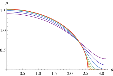
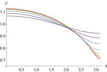
Figure 1: Plots of $\rho_{N}^{\text{sym}}(\theta,T)$ for $T=2$ (left), $T=5$ (right), and $N=3,5,10,25,50,100,250$ together with $\rho_{\infty}(\theta,T)$.

It turns out that the appropriate area variable for $\rho_{N}^{\text{sym}}$ is not $t=\lambda{\cal A}$ but $T=t(1-1/N)$ [5]. When $\rho^{\text{sym}}_{N}(\theta,T)$ is compared to $\rho^{\text{true}}_{N}(\theta,t)$, the $1/N$ correction in $t$ relative to $T$ has to be taken into account (so far, the size dependence of the $\rho_{N}^{\ell}$ has been suppressed).

The infinite-$N$ critical point is at $T=4$. For $T>4$, $\rho^{\text{sym}}_{N}(\theta,T)$ approaches $\rho_{\infty}(\theta,T)$ by power corrections in $1/N$ [5]. For $T<4$, $\rho_{\infty}(\theta,T)$ is zero for $|\theta|>\theta_{c}(T)$, where $0<\theta_{c}(T)<\pi$ and $\theta_{c}(4)=\pi$ (cf. Fig. 1). In this interval $\rho^{\text{sym}}_{N}(\theta,T)$ approaches zero by corrections that are exponentially suppressed in $N$.

The true eigenvalue density $\rho_{N}^{\text{true}}(\theta,t)$ has $N$ peaks (in the interval $[-\pi,\pi]$) and oscillates around $\rho_{N}^{\text{sym}}(\theta,T)$ (cf. [7]). Plots of $\rho_{N}^{\text{true}}(\theta,t)$ and $\rho_{N}^{\text{sym}}(\theta,T)$ are shown in Fig. 2 for $t=2$ and $t=5$.

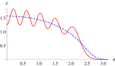
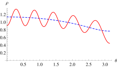
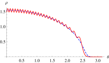
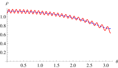
Figure 2: Plots of the densities $\rho_{N}^{\text{true}}(\theta,t)$ (red, solid) and $\rho_{N}^{\text{sym}}(\theta,T)$ (blue, dashed) for $t=2$ (left) and $t=5$ (right), $N=10$ (top), and $N=50$ (bottom).

3 Integral representations

The density $\rho_{N}^{\text{true}}$ can be obtained from the expectation value of [7]

$$R(u,v,W)=\frac{\det(1+uW)}{\det(1-vW)}=\sum_{p=0}^{N}\sum_{q=0}^{\infty}u^{p}v^{q}\chi_{p}^{A}(W)\chi_{q}^{S}(W)$$ (9)

with $|v|<1$. $\chi_{p}^{A}(W)$ (resp. $\chi_{q}^{S}(W)$) denotes the character of $W$ in a totally antisymmetric (resp. symmetric) representation. When we set $u=-v+\epsilon$ and expand to linear order in $\epsilon$, the LHS reads

$$R(-v+\epsilon,v,W)=1-\epsilon\Tr\frac{1}{v-W^{\dagger}}\,.$$ (10)

After decomposing the tensor product $p^{A}\otimes q^{S}$ into irreducible representations, we obtain for the expectation value of the trace (due to character orthogonality)

$$\bar{R}(v)\equiv\mathinner{\left\langle{\Tr\frac{1}{v-W^{\dagger}}}\right\rangle}=-\sum_{p=0}^{N-1}\sum_{q=0}^{\infty}(-1)^{p}v^{p+q}e^{-\frac{t}{2N}C(p,q)}d(p,q)\,,$$ (11)

where $C(p,q)$ and $d(p,q)$ denote the value of the quadratic Casimir and the dimension of the irreducible representation identified by the Young diagram

(12)

and are given by [9]

$$C(p,q) =(p+q+1)\left(N-\frac{p+q+1}{N}+q-p\right)\,,$$ (13)

$$d(p,q) =d^{A}(p)d^{S}(q)\frac{(N-p)(N+q)}{N}\frac{1}{p+q+1}\,,$$ (14)

$$d^{A}(p) ={N\choose p}\,,\qquad d^{S}(q)={N+q-1\choose q}.$$ (15)

We can exactly calculate sums of the form (with $|z|<1$)

$$\sum_{p=0}^{N-1}u^{p}d^{A}(p)(N-p)=N(1+u)^{N-1}\,,\quad\sum_{q=0}^{\infty}z^{q}d^{S}(q)(N+q)=\frac{N}{(1-z)^{N+1}}\,.$$ (16)

To factorize the sums over $p$ and $q$ in (11), we first write

$$\frac{1}{p+q+1}=\int_{0}^{1}d\rho\rho^{p+q}\,.$$ (17)

The $t$-dependent weight factor is the exponent of a bilinear form in $p$ and $q$ (given by (13)). By a Hubbard-Stratonovich transformation the dependence on $p$ and $q$ can be made linear. Performing the (independent) sums over $p$, $q$ then leads to [7]

$$\bar{R}(v) =-\frac{N^{2}}{t}e^{-\frac{t}{2}}\int\!\!\int_{-\infty}^{\infty}\frac{dxdy}{2\pi}\int_{0}^{1}d\rho\,e^{-\frac{N}{2t}(x^{2}+y^{2})+\frac{1}{2t}(x+iy)^{2}-\frac{1}{2}(x-iy)}$$

$$\quad\times\frac{\left[1-v\rho e^{-x-t/2}\right]^{N-1}}{\left[1-v\rho e^{iy-t/2}\right]^{N+1}}$$ (18)

(valid for $|v|<1$). Now the entire dependence on $N$ is explicit. The infinite-$N$ limit of $\rho_{N}^{\text{true}}$ can be obtained from this integral representation by using a saddle-point approximation for the integrals over $x$ and $y$ (cf. Sec. 5).

4 Asymptotic expansion of $\rho^{\text{sym}}_{N}$

An integral representation for $\psi^{(N)}(z)=\langle\det(z-W)^{-1}\rangle$, which determines $\rho^{\text{sym}}_{N}$, is obtained in a similar manner [5]. In this case, only a single integral is needed (valid for $|z|>1$),

$$\psi^{(N)}(z)=e^{\frac{NT}{8}}\sqrt{\frac{N}{2\pi T}}\int_{-\infty}^{\infty}du\,e^{-\frac{N}{2T}u^{2}}\left(ze^{-i\frac{u}{2}}-e^{i\frac{u}{2}}\right)^{-N}\,.$$ (19)

The aim of this section is to construct an asymptotic expansion of $\rho_{N}^{\text{sym}}(\theta,T)$ in powers of $1/N$ (cf. [7]). To this end we perform a saddle-point analysis of the integral in (19), from which $\rho_{N}^{\text{sym}}$ can be obtained via (5) and (6).

4.1 Saddle-point analysis

For $|z|=1$ the integrand of (19) has singularities on the real-$u$ axis. We therefore set $z=e^{\epsilon+i\theta}$, where $\epsilon>0$ ensures that $|z|>1$ but will later be taken to zero. The integrand of (19) can be written as $\exp(-Nf(u))$ with

$$f(u)=\frac{u^{2}}{2T}+\log\left(ze^{-i\frac{u}{2}}-e^{i\frac{u}{2}}\right)\,.$$ (20)

We now look for saddle points of the integrand in the complex-$u$ plane, which we label by $\bar{u}=iTU(\theta,T)$, where $U(\theta,T)=U_{r}(\theta,T)+iU_{i}(\theta,T)$ is a complex-valued function of $\theta$ and $T$. The saddle-point equation turns out to be

$$e^{-TU(\theta,T)}\frac{U(\theta,T)+1/2}{U(\theta,T)-1/2}=e^{\epsilon+i\theta}\,.$$ (21)

For $\epsilon=0$, this is equation (5.49) in [10] and is related to the inviscid complex Burgers equation via equation (5.44) there. In the present notation, the latter equation has the form

$$\frac{\partial U}{\partial T}+iU\frac{\partial U}{\partial\theta}=0\,.$$ (22)

Taking the absolute value of (21) leads to the equation

$$U_{i}^{2} =U_{r}\coth(TU_{r}+\epsilon)-U_{r}^{2}-\frac{1}{4}\,.$$ (23)

For $\epsilon=0$, this equation has been investigated previously in [10]. However, here we keep $\epsilon>0$ for the time being. The singularities of the integrand of (19) then all have $U_{r}<0$. Equation (23) describes one or more curves in the complex-$U$ plane on which the saddle points have to lie (for a given value of $\theta$, the saddles are isolated points on these curves).

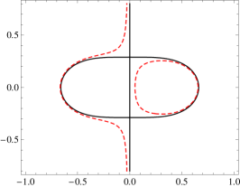
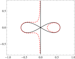
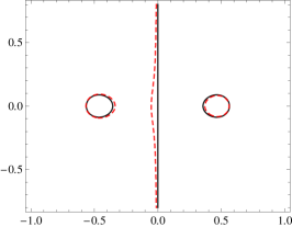
Figure 3: Examples of the contours in the complex-$U$ plane described by equation (23) for $T=3$ (left), $T=4$ (middle), and $T=5$ (right). The red dashed curves are for small $\epsilon>0$, while the black solid curves are for $\epsilon=0$. For our saddle-point analysis we keep $\epsilon>0$.

In Fig. 3 we show typical examples for these curves for $T<4$, $T=4$, and $T>4$, where $\epsilon$ has been chosen sufficiently close to zero. (The closed contours always enclose the points $U=1/2$ or $U=-1/2$. For $T>4$ and larger $\epsilon$, the closed contour in the left half-plane would be missing, but right now we are not concerned with this since we are only interested in the limit $\epsilon\to 0^{+}$.) Analyzing (21) numerically we find, for all values of $T$, that for a given value of $\theta$ there is always one (and only one) saddle point on the closed contour in the right half-plane, i.e., with $U_{r}>0$. Note that we are showing the complex-$U$ plane, in which the original integration contour corresponds to the imaginary axis. The integration contour can be smoothly deformed to go through the (single) saddle point in the right half-plane along a path of steepest descent. No singularities are crossed since they all have $U_{r}<0$. There are also saddle points on the contour(s) in the left half-plane (in fact, there are infinitely many on the open contour), but these need not be considered. Figure 4 shows an example for the location of the saddle points and the deformation of the integration contour in the complex-$u$ plane.

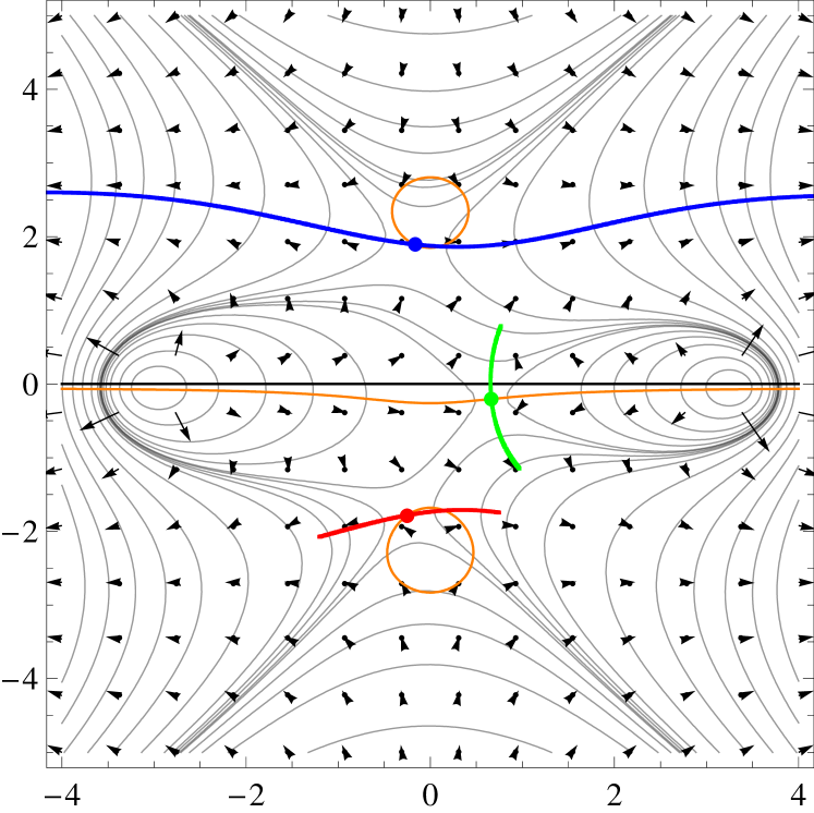
Figure 4: Example for the location of the saddle points and the deformation of the integration contour in the complex-$u$ plane for $T=5$ and $\theta=3$ (with small $\epsilon>0$). The thin solid lines are lines of constant $\operatorname{Re}f(u)$, the arrows point in the direction of increasing $\operatorname{Re}f(u)$. On each of the closed orange curves there is one saddle point (red dot and blue dot), and on the open orange curve there are infinitely many saddle points, but only one of them in the region shown in the plot (green dot). The thick blue curve is the integration path along the direction of steepest descent through the relevant saddle point.

Once the integration contour has been deformed to go through the saddle point, we can safely take the limit $\epsilon\to 0^{+}$. Parametrizing the contour in the vicinity of the saddle point by $u=\bar{u}+xe^{i\beta}$, where $x$ is the new integration variable corresponding to the fluctuations around the saddle and $\beta$ is the angle which the path of steepest descent makes with the real-$u$ axis, $\psi^{(N)}(e^{i\theta},T)$ is given, up to exponentially small corrections in $N$, by

$$\psi^{(N)}(e^{i\theta},T) =\frac{1}{2^{N}}\sqrt{\frac{N}{2\pi T}}\,e^{\frac{NT}{8}-i\frac{N\theta}{2}+i\beta}\int_{-\infty}^{\infty}dx\,e^{-Ng(x)}\,,$$ (24)

$$g(x) =\frac{1}{2T}\bigl{(}xe^{i\beta}+iTU(\theta,T)\bigr{)}^{2}+\log\sinh\frac{i\theta-ixe^{i\beta}+TU(\theta,T)}{2}\,.$$ (25)

We can now expand $g(x)$ in $x$. The linear order vanishes by construction. The second order gives a Gaussian integral over $x$, resulting in

$$\psi^{(N)}(e^{i\theta},T) \approx e^{\frac{NT}{8}+\frac{NTU^{2}(\theta,T)}{2}}\frac{\left[e^{-i\theta}(1/4-U^{2}(\theta,T))\right]^{N/2}}{\sqrt{1-T(1/4-U^{2}(\theta,T))}}\,.$$ (26)

Note that the factor $e^{-i\theta}$ cannot be pulled out of the term in square brackets because periodicity in $\theta$ would be lost.

There is a potential complication. In principle, $g^{\prime\prime}(0)$ and therefore the denominator in (26) could be zero, which would mean that the integral over $x$ cannot be performed in Gaussian approximation. For $T>4$, it is straightforward to show that $g^{\prime\prime}(0)$ is never zero. For $T\leq 4$, one can use (21) to show that $g^{\prime\prime}(0)=0$ only for the saddle points corresponding to the two angles $\theta=\pm\theta_{c}(T)$ at which $\rho_{\infty}(\theta,T)$ becomes zero (see section 2). This means that for $|\theta|=\theta_{c}(T)$ the asymptotic expansion in $1/N$ diverges, and that it converges ever more slowly as $|\theta|\to\theta_{c}$ from below.

Note that for $T<4$ and $\theta_{c}(T)\leq|\theta|\leq\pi$ the function $\rho^{\text{sym}}_{N}(\theta,T)$ is exponentially suppressed in $N$. The study of the large-$N$ asymptotic behavior in this region requires more work.

4.2 Leading-order result

Equation (26) is the leading order in the $1/N$ expansion of $\psi^{(N)}(e^{i\theta},T)$. We now show that it leads to $\rho_{N}^{\text{sym}}(\theta,T)\to\rho_{\infty}(\theta,T)$ as $N\to\infty$. We first write (26) in the form

$$\frac{1}{N}\log\psi^{(N)}(e^{i\theta},T)=\frac{T}{8}-f(\bar{u})+\mathcal{O}(1/N)\,.$$ (27)

Note that in this order we do not need the denominator in (26), which corresponds to $f^{\prime\prime}(\bar{u})$ (or $g^{\prime\prime}(0)$). Using $\bar{u}=iTU$ this leads to

$$G^{\text{sym}}_{N}(z)=\frac{1}{z-e^{-TU}}+\mathcal{O}(1/N)=\frac{1}{z}\left(U+\frac{1}{2}\right)+\mathcal{O}(1/N)$$ (28)

where in the last step we have used the saddle-point equation (21). Equation (6) then gives

$$\lim_{N\to\infty}\rho_{N}^{\text{sym}}(\theta,T)=2\operatorname{Re}U(\theta,T)\,,$$ (29)

which equals $\rho_{\infty}(\theta,T)$ of DO [1, 11] since $U(\theta,T)$ satisfies (21) (which leads to (45) below with $\lambda=U-1/2$ and $v=1/z$).

4.3 $1/N$ correction to $\rho_{\infty}$

Higher-order terms in the $1/N$ expansion of $\psi^{(N)}(e^{i\theta},T)$ can be obtained in the standard way by considering higher powers of $x$ in the expansion of $g(x)$, resulting in integrals of the type $\int_{-\infty}^{\infty}dx\,x^{2n}e^{-g^{\prime\prime}(0)x^{2}/2}$ with $n\in\mathbb{N}$. However, if we are only interested in the $1/N$ correction to $\rho_{\infty}(\theta,T)$ the result (26) is already sufficient ($1/N$ corrections to this result would give $1/N^{2}$ corrections to $\rho_{\infty}(\theta,T)$). Therefore we now write

$$\frac{1}{N}\log\psi^{(N)}(e^{i\theta},T)=\frac{T}{8}-f(\bar{u})-\frac{1}{2N}\log[Tf^{\prime\prime}(\bar{u})]+\mathcal{O}(1/N^{2})\,,$$ (30)

which leads to

$$\rho_{N}^{\text{sym}}(\theta,T)=2\operatorname{Re}\left[U\left(1+\frac{1}{N}\frac{T(1/4-U^{2})}{[1-T(1/4-U^{2})]^{2}}\right)\right]+\mathcal{O}(1/N^{2})\,.$$ (31)

Note that for $T\leq 4$ and $|\theta|\to\theta_{c}(T)$ (from below) the denominator of the $1/N$ term approaches zero, which corresponds to the complication discussed in section 4.1. Note also that for $T\leq 4$ and $|\theta|>\theta_{c}$ the saddle point $U(\theta,T)$ is purely imaginary so that both the leading order and the $1/N$ term are zero. This confirms that the above saddle-point analysis is not the right tool to compute finite-$N$ effects in this region.

In Fig. 5 we show examples for the $1/N$ corrections to $\rho_{\infty}(\theta,T)$ for $N=10$ and $T=2$ and $5$.

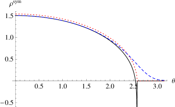
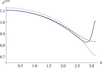
Figure 5: Examples for the $1/N$ corrections to $\rho_{\infty}(\theta,T)$ for $N=10$, $T=2$ (left), and $T=5$ (right). Shown are the exact result for $\rho_{N}^{\text{sym}}(\theta,T)$ (blue dashed curve), the infinite-$N$ result $\rho_{\infty}(\theta,T)$ (red dotted curve), and the asymptotic expansion of $\rho_{N}^{\text{sym}}(\theta,T)$ up to order $\mathcal{O}(1/N)$ (black solid curve). We observe that the asymptotic expansion converges rapidly for small $|\theta|$ and more slowly for larger $|\theta|$.

5 Saddle-point analysis for $\rho^{\text{true}}_{N}$

We now turn to the integral representation (18) to take the first steps in a $1/N$ expansion of $\rho^{\text{true}}_{N}(\theta,t)$ (cf. [7]). Since this integral representation was derived for $|v|<1$, we set $v=e^{i\theta-\epsilon}$ with $|\theta|\leq\pi$, $\epsilon>0$, and take the limit $\epsilon\to 0$ at the end. We write (18) as

$$\bar{R}(v) =-\frac{N^{2}}{t}e^{-\frac{t}{2}}\int\!\!\int_{-\infty}^{\infty}\frac{dxdy}{2\pi}\int_{0}^{1}d\rho\,e^{-\frac{N}{2t}\left(x^{2}+y^{2}\right)+\frac{1}{2t}(x+iy)^{2}-\frac{1}{2}(x-iy)}$$ (32)

$$\quad\times e^{(N-1)\log\left(1-v\rho e^{-x-t/2}\right)-(N+1)\log\left(1-v\rho e^{iy-t/2}\right)}\,.$$ (33)

At large $N$, the integrals over $x$ and $y$ decouple at leading order and can be done independently by saddle-point approximations. Let us start with the integral over $y$ since it is conceptually simpler. The $y$-dependent coefficient of the term in the exponent in equation (32) that is proportional to $-N$ is

$$\bar{f}(y)=\frac{1}{2t}y^{2}+\log\left[1-v\rho e^{iy-\frac{t}{2}}\right]\,.$$ (34)

Substituting $y=u-it/2=it(U-1/2)$ (with $u=itU$ in analogy to section 4) results in exactly the same integrand that was already considered in section 4, with the replacements $T\to t$ and $z\to 1/v\rho$ (with $|v\rho|<1$) and with an integration over $u$ that is now along the line from $-\infty+it/2$ to $+\infty+it/2$. Since there are no singularities between this line and the real-$u$ axis we can change the integration path to be along the real-$u$ (or imaginary-$U$) axis. Now everything goes through as in section 4. The saddle-point equation reads

$$e^{-tU}\frac{U+1/2}{U-1/2}=\frac{1}{v\rho}\,,$$ (35)

which is equivalent to (21). In Fig. 6 we show the contours in the complex-$U$ plane on which the solutions of the saddle-point equation have to lie. (For sufficiently small $\rho$ we now encounter the case mentioned in section 4.1 where for $t>4$ the closed contour in the left half-plane is missing.) The relevant saddle point, which we denote by $y_{0}(\theta,t,\rho)$, is again on the closed contour in the right half-plane. For decreasing $\rho$ this contour contracts, but this makes no difference to our analysis. The result for the $y$-integral is given by an expression similar to (26).

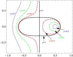
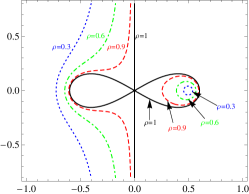
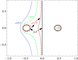
Figure 6: Contours of solutions of equation (35) in the complex-$U$ plane at $t=3$ (left), $t=4$ (middle), and $t=5$ (right) for $\rho=1$ (black, solid), $\rho=0.9$ (red, dashed), $\rho=0.6$ (green, dot-dashed), and $\rho=0.3$ (blue, dotted). In the figures (but not in the analysis) we have taken $|v|=1$ for simplicity.

We now turn to the integral over $x$. The $x$-dependent coefficient of the term in the exponent in equation (32) that is proportional to $-N$ is

$$\tilde{f}(x)=\frac{1}{2t}x^{2}-\log\left[1-v\rho e^{-x-t/2}\right]=-\bar{f}(ix)\,.$$ (36)

Substituting $x=-iu-t/2=t(U-1/2)$ (with $u=itU$) again leads to the integral considered in section 4 and the saddle-point equation (35), except that the integration is now along the real-$U$ axis. The positions of the saddle points of the $x$-integral are obtained by rotating the saddles of the $y$-integral by $-\pi/2$ in the complex-$U$ plane, i.e., $x_{s}=-iy_{s}$. At a saddle point we have

$$\tilde{f}^{\prime\prime}(x_{s})=\frac{1}{t}+\frac{x_{s}}{t}\left(1+\frac{x_{s}}{t}\right)=\bar{f}^{\prime\prime}(y_{s})\,,$$ (37)

and therefore the directions of steepest descent through a saddle $y_{s}$ and the corresponding saddle $x_{s}=-iy_{s}$ are identical (no rotation). By analyzing the directions along which the phase of the integrand is constant, we find that the integration contour can always be deformed to go through the (single) saddle point in the right half-plane in the direction of steepest descent. Depending on the parameters $\rho$, $v$, and $t$, there is either one or no additional saddle point on the contour(s) in the left half-plane through which we can also go in the direction of steepest descent. If there is such an additional saddle point, we find that its contribution to the integral is always exponentially suppressed in $N$ compared to the saddle point in the right half-plane and can therefore be dropped from the saddle-point analysis. In addition, there are infinitely many more saddle points on the open contour in the left half-plane. However, we cannot deform the integration path to go through these points in the direction of steepest descent and therefore do not need to include them. An example for the location of the saddle points and the deformation of the integration path is given in Fig. 7. To summarize, the $x$-integral can be approximated by the contribution of the single saddle point in the right half-plane, which again leads to an expression similar to (26).

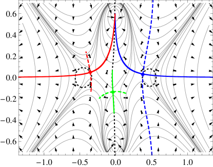
Figure 7: Example for the location of the saddle points and the deformation of the integration path in the complex-$U$ plane for $t=5$ and $\rho=0.95$. The dashed black curves (two closed, one open) are the curves on which all saddle points have to lie, cf. (23). In this example $\theta=3.0$. On each of the closed curves there is one saddle point (red dot and blue dot), and on the open curve there are infinitely many saddle points, but only one of them in the region shown in the plot (green dot). The thin solid lines are lines of constant $\operatorname{Re}\tilde{f}(x)$ and $\operatorname{Re}\bar{f}(y)$. The arrows point in the direction of increasing $\operatorname{Re}\tilde{f}(x)$ or decreasing $\operatorname{Re}\bar{f}(y)$. The dashed blue curve is the integration path for the $y$-integral along the direction of steepest descent. The solid red-blue curve is the integration path for the $x$-integral along the direction of steepest descent.

Combining the saddle-point approximations for the integrals over $x$ and $y$, we find that, up to exponentially small corrections in $N$, the integral in equation (32) is given by

$$\bar{R}(v)=-\frac{N^{2}}{t}e^{-t/2}\int_{0}^{1}d\rho\,\frac{1}{2\pi}\left(\frac{2\pi}{N\tilde{f}^{\prime\prime}(x_{0})}\right)\frac{1}{(1-v\rho e^{-x_{0}-t/2})^{2}}\,e^{-x_{0}}\,,$$ (38)

where $x_{0}=x_{0}(\theta,t,\rho)$ is the dominating saddle point of the $x$-integral. $x_{0}$ is a solution of the saddle-point equation obtained by differentiating $\tilde{f}(x)$, which can be written as

$$v\rho e^{-x_{0}-t/2}=\frac{x_{0}}{x_{0}+t}$$ (39)

and leads to

$$\left(1-v\rho e^{-x_{0}-\frac{t}{2}}\right)^{2}=\left(\frac{t}{t+x_{0}}\right)^{2}\,.$$ (40)

With (37) we obtain

$$\tilde{f}^{\prime\prime}(x_{0})\left(1-v\rho e^{-x_{0}-\frac{t}{2}}\right)^{2}=\frac{t+x_{0}\left(t+x_{0}\right)}{\left(t+x_{0}\right)^{2}}$$ (41)

and

$$\bar{R}(v)=-\frac{N}{t}e^{-\frac{t}{2}}\int_{0}^{1}d\rho\,\frac{\left(t+x_{0}\right)^{2}}{t+x_{0}\left(t+x_{0}\right)}\,e^{-x_{0}}\,.$$ (42)

Differentiating equation (39) with respect to $\rho$ leads to

$$\frac{\partial x_{0}}{\partial\rho} =\frac{1}{\rho}\frac{x_{0}\left(t+x_{0}\right)}{t+x_{0}\left(t+x_{0}\right)}=ve^{-x_{0}-t/2}\frac{\left(t+x_{0}\right)^{2}}{t+x_{0}\left(t+x_{0}\right)}\,,$$ (43)

which yields

$$\bar{R}(v)=-\frac{N}{tv}\int_{0}^{1}d\rho\,\frac{\partial x_{0}}{\partial\rho}=-\frac{N}{tv}\left[x_{0}(\theta,t,\rho=1)-x_{0}(\theta,t,\rho=0)\right]\,.$$ (44)

We know from (39) that $x_{0}(\theta,t,\rho=0)=0$. If we parametrize $x_{0}(\theta,t,\rho=1)=\lambda(\theta,t)t$, where $\lambda(\theta,t)$ has to solve

$$\lambda=\frac{1}{\frac{1}{v}e^{t\left(\lambda+1/2\right)}-1}\,,$$ (45)

and take the limit $\epsilon\to 0^{+}$, we end up with

$$\bar{R}(v)=-\frac{N\lambda(\theta,t)}{v}\,,\qquad v=e^{i\theta}\,.$$ (46)

Here we need to keep in mind that we have to pick the solution of equation (45) which corresponds to the dominating saddle point $x_{0}$ of the $x$-integral for $|v\rho|<1$.

Using (6) and

$$G(z)=\frac{1}{z}-\frac{1}{z^{2}N}\bar{R}\left(z^{-1}\right)$$ (47)

we obtain

$$\lim_{N\to\infty}\rho_{N}^{\text{true}}(\theta,t)=1+2\operatorname{Re}\lambda(\theta,t)\,,$$ (48)

which is equal to $\rho_{\infty}(\theta,t)$ [1, 11]. Keeping higher orders in the saddle-point approximation (as explained in section 4.3), we can compute the asymptotic expansion of $\rho_{N}^{\text{true}}(\theta,t)$ in powers of $1/N$.

6 Conclusions

The probability distribution of Wilson loops in $\text{SU}(N)$ YM in two Euclidean dimensions can be written as a sum over irreducible representations (where only dimension, second-order Casimir, and character of $W$ enter). This allows for the derivation of integral representations for different density functions (including the true eigenvalue density), which have the same infinite-$N$ limit. These integral representations, where $N$ enters only as a parameter, are exact for any finite $N$. Results at infinite $N$ can be obtained by saddle-point approximations. Next-order terms in an expansion in $1/N$ give reasonable results in the interval where $\rho_{\infty}(\theta)>0$. More work is needed to get finite $N$ effects where $\rho_{\infty}(\theta)=0$ and corrections are exponentially suppressed in $N$.

7 Acknowledgments

I would like to thank Herbert Neuberger and Tilo Wettig. The presented work has been done in close collaboration with them. I acknowledge support by BayEFG and the DOE under grant number DE-FG02-01ER41165 at Rutgers University.

References

- [1] B. Durhuus and P. Olesen. The spectral density for two-dimensional continuum QCD. Nucl. Phys., B184:461, 1981.
- [2] R. Narayanan and H. Neuberger. Universality of large N phase transitions in Wilson loop operators in two and three dimensions. JHEP, 12:066, 2007.
- [3] R. Narayanan, H. Neuberger, and E. Vicari. A large N phase transition in the continuum two dimensional SU(N) X SU(N) principal chiral model. JHEP, 04:094, 2008.
- [4] H. Neuberger. Burgers’ equation in 2D SU(N) YM. Phys. Lett., B666:106–109, 2008.
- [5] H. Neuberger. Complex Burgers’ equation in 2D SU(N) YM. Phys. Lett., B670:235–240, 2008.
- [6] J.-P. Blaizot and M. A. Nowak. Large confinement and turbulence. Phys. Rev. Lett., 101:102001, 2008.
- [7] R. Lohmayer, H. Neuberger, and T. Wettig. Eigenvalue density of Wilson loops in 2D SU(N) YM. JHEP, 05:107, 2009.
- [8] D. J. Gross and W. Taylor. Two-dimensional QCD is a string theory. Nucl. Phys., B400:181–210, 1993.
- [9] A. M. Perelomov and V. M. Popov. Casimir operators for the unitary group. JETP Letters, 1:160–162, 1965.
- [10] R. Lohmayer, H. Neuberger, and T. Wettig. Possible large-N transitions for complex Wilson loop matrices. JHEP, 11:053, 2008.
- [11] R. A. Janik and W. Wieczorek. Multiplying unitary random matrices – universality and spectral properties. J. Phys. A: Math. Gen., 37:6521–6529, 2004.