Spectrum of Perturbations in Anisotropic Inflationary Universe with Vector Hair

Burak Himmetoglu School of Physics and Astronomy, University of Minnesota, Minneapolis, MN 55455, USA
Abstract

We study both the background evolution and cosmological perturbations of anisotropic inflationary models supported by coupled scalar and vector fields. The models we study preserve the U(1)𝑈1U(1) gauge symmetry associated with the vector field, and therefore do not possess instabilities associated with longitudinal modes (which instead plague some recently proposed models of vector inflation and curvaton). We first intoduce a model in which the background anisotropy slowly decreases during inflation; we then confirm the stability of the background solution by studying the quadratic action for all the perturbations of the model. We then compute the spectrum of the h×subscripth_{\times} gravitational wave polarization. The spectrum we find breaks statistical isotropy at the largest scales and reduces to the standard nearly scale invariant form at small scales. We finally discuss the possible relevance of our results to the large scale CMB anomalies.

preprint: UMN-TH-2821/09preprint: ArXiv:0910.3235

I Introduction

The inflationary paradigm has become a widely accepted description of the early universe, which has been successful in solving the classical problems of FRW cosmology Guth ; Linde . Moreover, inflation provides a mechanism for generation of nearly scale invariant spectrum of perturbations that can seed the structure we observe today mfb . Inflationary era is characterized by a quasi de-Sitter expansion with a nearly constant Hubble rate. During inflation, quantum fluctuations are generated and amplified to scales above the Hubble scale (which specifies the horizon of casual processes) where they remain frozen until they re-enter the horizon after inflation has ended. A key assumption about the quantum fluctuations during the quasi de-Sitter stage is that they are in an adiabatic vacuum stage in the deep sub-horizon (early time) regime, which results in a nearly scale invariant spectrum.

Results of the WMAP experiment WMAP are in overall agreement with the predictions of inflation. However, certain features of the full sky CMB maps seem to be anomalous in the standard picture. These anomalies include the low power in the quadrupole moment lowl , the alignment of the lowest multipole moments (known as the ’axis-of-evil’) axis , and an asymmetry in power between the northern and southern ecliptic hemispheres asym . The statistical significance of these anomalies has been extensively discussed in the literature and despite numerous efforts, an explanation due to a systematic effect or a foreground signal affecting the analysis is not forthcoming. These anomalies suggest a violation of statistical isotropy of cosmological fluctuations, which is at odds with standard mechanisms of generation of perturbations in inflationary models. Therefore, the possibility of relating the anomalies with modifications in the standard inflationary picture has been considered by numerous authors recently.

In the standard picture, almsubscript𝑎𝑙𝑚a_{lm} coefficients of CMB temperature anisotropies satisfy <almalm>=Clδllδmmexpectationsubscript𝑎𝑙𝑚superscriptsubscript𝑎𝑙𝑚subscript𝐶𝑙subscript𝛿𝑙superscript𝑙subscript𝛿𝑚superscript𝑚<a_{lm}\,a_{lm}^{*}>=C_{l}\,\delta_{ll^{\prime}}\,\delta_{mm^{\prime}} (so, the temperature fluctuations are said to be statistically isotropic). It has been shown in gcp ; gcp2 that an anisotropic expansion that took place at the onset of standard single field inflation, leads to a nonvanishing correlation of the almsubscript𝑎𝑙𝑚a_{lm} coefficients for different l𝑙l-modes. This violation of statistical isotropy might then be related to the alignment of the lowest multipoles observed in the CMB data. Therefore, several authors considered inflationary models with an anisotropic stage. As the simplest possible modification, anisotropic initial conditions at the onset of single field inflation have been considered in references gcp ; gcp2 ; uzan1 ; uzan2 . Isotropization of the universe takes place due to the fast expansion supported by the inflaton field. Fluctuations at scales comparable to the horizon scale during the anisotropic stage of inflation are sensitive to the background evolution and thus provide breaking of statistical isotropy at those scales. If inflation had a limited duration, this could leave an imprint on the largest observable scales. On the other hand, fluctuations that leave the horizon after isotropization re-enter earlier than modes that left the horizon during the anisotropic stage, producing the standard nearly scale invariant spectrum at small scales 111It was also shown in gkp that the anisotropic stage could lead to a detectable gravitational wave signal.. Since in such models isotropy is reached very soon (within one Hubble time) the breaking of statistical isotropy can be visible if the total duration of inflation is tuned to only the minimal duration to solve the standard problems of FRW cosmology.

The fine-tuning can be relaxed if the anisotropic stage is prolonged, due to the existence of other sources, for example vector fields. Recently, anisotropic expansion driven by vector fields have been studied by many authors. The anisotropic expansion is achieved when the vector field acquires a nonzero vacuum expectation value (VEV) along a spatial direction. There is a range of models which differ by the way the VEV is obtained. The first anisotropic inflationary model was considered long ago in reference ford , where the U(1)𝑈1U(1) symmetry of the vector field action is broken by a potential term, which needs to have a negative curvature to support an anisotropic expansion. It has been shown in reference hcp1 that this model is plagued by a ghost instability, and its quantum theory is inconsistent 222One may hope that this model has a well behaved UV completion. However, inflationary predictions are sensitive to this high energy regime, where the completion is needed.. In another model, the ACW model acw , the VEV is obtained by a lagrange multiplier field which fixes the norm of the vector field and breaks the U(1)𝑈1U(1) gauge symmetry. The stability analysis of the ACW model by considering the most general perturbations of the background has been performed in references dgw and hcp1 ; hcp2 . In the latter studies, it has been shown that the linearized perturbations diverge close to horizon crossing, indicating the instability of the background solution. Another model soda1 considered a nonminimal coupling of the vector field to the scalar curvature which breaks the conformal invariance of the vector field action. The coupling with curvature allows for a slow-roll phase during the prolonged anisotropic expansion, and the universe isotropizes due to the existence of a massive scalar field, which is responsible for the overall isotropic expansion of the universe. Models of inflation with nonmininal coupling to curvature have also been considered for standard isotropic inflation mukhvect . Isotropy of space is realized if 3N3𝑁3N mutually orthogonal vector fields have equal VEVs. Instead, for randomly oriented N𝑁N vector fields, one expects a statistically isotropic background with order 1/N1𝑁1/\sqrt{N} anisotropy. Perturbative calculations based around such a background configuration have been considered in references Golovnev:2008hv ; Golovnev:2009ks ; Golovnev:2009rm and in hcp3 . The latter study is the only complete study linearized study of perturbations, taking into account all the physical degrees of freedom, and coupling between vector field and metric perturbations. It has been shown in hcp3 that the equations of motion for the linearized perturbations become singular close to horizon crossing, leading to instabilities. In all of these models (including acw ; soda1 ; mukhvect ), instabilities are related to the existence of the longitudinal polarization of the vector field (which would otherwise be absent when the U(1)𝑈1U(1) symmetry is restored), which becomes a ghost close to horizon crossing (In the vector inflation model mukhvect , ghosts also appear in the deep UV regime).

More recently, reference Watanabe:2009ct introduced an anisotropic inflation model driven simultaneously by a vector field and a massive scalar field. The vector field is massless, but it is coupled to the scalar field through its kinetic term. Such type of coupling preserves the U(1)𝑈1U(1) gauge invariance of the vector field, so that the dangerous longitudinal vector polarization is absent; moreover the conformal invariance of the vector field is broken. When the vector field has a nonvanishing VEV along a spatial direction, the model possess an anisotropically expanding attractor solution. The anisotropy in the attractor is initially small, but it increases towards the end of inflation; therefore this is a counter example to the cosmic no hair conjecture (See Kaloper:1991rw for a different example) .The breaking of conformal invariance due to the scalar-vector coupling can also be used to generate magnetic fields from inflation, as discussed in reference Turner:1987bw and more recently in Gordon:2000hv ; Demozzi:2009fu and Watanabe:2009ct . These models are expected to be free from ghost instabilities as long as the coupling to the scalar field remains positive. However to our knowledge, there has been no complete study of the stability of these models, which take into account all the physical degrees of freedom of the system (including gravity). A complete study of stability is therefore necessary, given the problems identified with other vector field models hcp1 ; hcp2 ; hcp3 .

In this work, we will present a complete study of cosmological perturbations of models with scalar-vector coupling that lead to an anisotropically expanding Bianchi-I background solution. We will also consider generalizations of the original model introduced in Watanabe:2009ct , to include additional scalar fields, so that isotropization can be achieved before the end of inflation. This is required in order to obtain a scale invariant spectrum of perturbations at small scales, but the large scale spectrum is modified, which in turn can be related to the CMB anomalies. Our study has two main steps: one is to show that the model is free of ghost instabilities, and the second is to study the resulting phenomenology. We perform the first step explicitly in this paper. We develop the necessary tools to study the phenomenology of the model and as a simple exercise, we study only the spectrum of h×subscripth_{\times} gravitational wave polarization in this paper. The study of the full phenomenology (including the spectrum of the curvature perturbation) will be communicated elsewhere me .

We will follow the formalism developed in gcp2 ; hcp2 to decompose and classify the perturbations. The generic background metric we study is the Bianchi-I metric with a residual two dimensional isotropy, given by

ds2=dt2+a(t)2dx2+b(t)2(dy2+dz2)𝑑superscript𝑠2𝑑superscript𝑡2𝑎superscript𝑡2𝑑superscript𝑥2𝑏superscript𝑡2𝑑superscript𝑦2𝑑superscript𝑧2ds^{2}=-dt^{2}+a(t)^{2}\,dx^{2}+b(t)^{2}\,\left(dy^{2}+dz^{2}\right)

We exploit the two dimensional isotropy of the yz𝑦𝑧y-z plane to decompose the perturbations into two decoupled classes: 2d2𝑑2d scalar modes and 2d2𝑑2d vector modes (As discussed in gcp2 , there is no two dimensional transverse-traceless mode). The linearized Einstein equations and the quadratic action for the two types of modes are decoupled and therefore we study them separately. We can deduce the number of degrees of freedom coming from each of the fields (gravity+vector field+scalar field) by a simple counting, which does not depend on the decomposition chosen to classify them. The metric has 101010 perturbations (δgμν𝛿subscript𝑔𝜇𝜈\delta g_{\mu\nu}) to start with, 4 of which can be removed by coordinate transformations. Of the remaining 6 modes, 4 are nondynamical, which can be best understood from the ADM formalism adm . In the ADM formalism, the gravitational action is decomposed into the dynamical part containing the spatial metric hijsubscript𝑖𝑗h_{ij} and a part containing the lapse (N) and shift functions (Nisubscript𝑁𝑖N_{i}). The lapse and shift functions have no kinetic terms in the action, and they can be integrated out by solving their equations of motion 333The equations of motion derived from extremezing the gravitational action with respect to lapse and shift functions result in the momentum and hamiltonian constraints.. This leaves only hijsubscript𝑖𝑗h_{ij} as dynamical modes, which have only two degrees of freedom. In summary, the metric perturbations have only 2 dynamical degrees of freedom (which are the gravitational wave polarizations in the standard case) and 4 nondyncamical modes. For the case of the vector field, out of 4 perturbations to start with (δAμ𝛿subscript𝐴𝜇\delta A_{\mu}), one perturbation can be removed by the U(1)𝑈1U(1) gauge transformation. Out of the remaining 3 perturbations 2 of them are dynamical and one mode is nondyamical (δA0𝛿subscript𝐴0\delta A_{0}). The scalar field perturbation introduces a single dynamical degree of freedom. Therefore, in total, the perturbations comprise of 5 dynamical modes, 2 of which are 2d2𝑑2d vector and 3 are 2d2𝑑2d scalar modes. When additional scalar fields are considered, each field introduces an extra scalar dynamical degree of freedom.

We will insert the perturbative expansion of the metric, the vector field and the scalar field(s) into the starting action and expand it at the quadratic order. We will show that the actions for the 2d2𝑑2d vector and 2d2𝑑2d scalar modes are decoupled, so we study them separately. We will determine the linear combinations of perturbations that canonically normalize the action, generalizing the computation of the standard isotropic case musa . The study of the quadratic action is crucial for both showing that the model is consistent (free of ghosts) and also for determining the initial conditions for the perturbations. For modes that are inside the horizon, canonical combinations of perturbations can be quantized, and initial conditions can be set by the canonical commutation relations and by the requirement that the adiabatic vacuum state has minimal energy. We then proceed by numerically integrating the evolution equations for the canonical fields, starting from adiabatic initial conditions deep inside the horizon, until the end of inflation, which gives us the primordial power spectra. We do so for the 2d2𝑑2d vector modes in this paper (which will be related to the power spectrum of the h×subscripth_{\times} polarization of gravitational waves) and perform the study of the spectrum of 2d2𝑑2d scalar modes in a separate publication.

The paper is organized as follows: In section II, we summarize the anisotropic inflationary background solution obtained in reference Watanabe:2009ct and generalize the model to possess extra scalar fields. This generalization leads to isotropization before the end of inflation. In section III, we discuss the perturbations around the background configuration. Specifically, in subsection III.1, we review and discuss the decomposition of perturbations around the Bianchi-I background solution, following the formulation of reference gcp2 . In subsection III.2, we discuss the generic properties of coupled vector-scalar models and develop tools that we will use in the following sections in order to find adiabatic initial conditions for such systems.

In subsection III.3 we discuss 2d2𝑑2d vector perturbations around the background configuration. We compute the action for 2d2𝑑2d vector modes and find the combinations of perturbations that canonically normalize the action. In section IV, we compute the power spectra of the 2d2𝑑2d vector modes numerically. This study results in the spectrum of h×subscripth_{\times} gravitational wave mode. We show that the spectrum has angular dependence (so breaks statistical isotropy) at large scales and reduces to the standard nearly scale invariant form at small scales. We also provide a fit to the numerically obtained spectrum. Finally in section V we provide a general discussion about the results we have obtained and their possible relation to observations.

We also provide two extensive appendices: In appendix VI.1, we derive the relation between the 2d2𝑑2d decomposed modes and the standard longitudinal mode, which has been used to determine the power spectra. In appendix VI.2, we perform the study of the 2d2𝑑2d scalar modes. More precisely, we compute the quadratic action and determine the modes that canonically normalizes the action. The spectrum of scalar perturbations and the consequent phenomenological predictions (specifically, the <almalm>expectationsubscript𝑎𝑙𝑚superscriptsubscript𝑎superscript𝑙superscript𝑚<a_{lm}\,a_{l^{\prime}m^{\prime}}^{*}> correlation) will be presented elsewhere.

II Anisotropic inflationary expansion due to coupled vector and scalar fields

The models we discuss in this work are generically described by the following action

S=d4xg[Mp22Ra=1N(12μϕaμϕa+Va(ϕa))12μϕμϕV(ϕ)14f2(ϕ)FμνFμν]𝑆superscript𝑑4𝑥𝑔delimited-[]superscriptsubscript𝑀𝑝22𝑅superscriptsubscript𝑎1𝑁12subscript𝜇subscriptitalic-ϕ𝑎superscript𝜇subscriptitalic-ϕ𝑎subscript𝑉𝑎subscriptitalic-ϕ𝑎12subscript𝜇italic-ϕsuperscript𝜇italic-ϕ𝑉italic-ϕ14superscript𝑓2italic-ϕsubscript𝐹𝜇𝜈superscript𝐹𝜇𝜈S=\int\,d^{4}x\,\sqrt{-g}\,\left[\frac{M_{p}^{2}}{2}\,R-\sum_{a=1}^{N}\,\left(\frac{1}{2}\,\partial_{\mu}\phi_{a}\,\partial^{\mu}\phi_{a}+V_{a}(\phi_{a})\right)-\frac{1}{2}\,\partial_{\mu}\phi\,\partial^{\mu}\phi-V(\phi)-\frac{1}{4}\,f^{2}(\phi)\,F_{\mu\nu}\,F^{\mu\nu}\right] (1)

The original discussion of these coupled vector-scalar field theories in an anisotropic inflationary background was given in Watanabe:2009ct , where there is only the single scalar field ϕitalic-ϕ\phi in the action. We assume that only one of the scalar fields (or only one linear combination) enters in the kinetic function f𝑓f for the vector field. We denote the remaining scalars with ϕasubscriptitalic-ϕ𝑎\phi_{a} (a=1,,N)𝑎1𝑁(a=1,\dots,N). The metric ansatz is taken to be the homogeneous but anisotropic Bianchi-I metric given by

ds2=dt2+e2α(t)[e4σ(t)dx2+e2σ(t)(dy2+dz2)]𝑑superscript𝑠2𝑑superscript𝑡2superscript𝑒2𝛼𝑡delimited-[]superscript𝑒4𝜎𝑡𝑑superscript𝑥2superscript𝑒2𝜎𝑡𝑑superscript𝑦2𝑑superscript𝑧2ds^{2}=-dt^{2}+e^{2\alpha(t)}\,\left[e^{-4\sigma(t)}\,dx^{2}+e^{2\sigma(t)}\,\left(dy^{2}+dz^{2}\right)\right] (2)

In the above metric α𝛼\alpha measures the number of e-folds of average isotropic expansion of the universe and σ𝜎\sigma measures the deviation from anisotropy. This metric also possesses a left over 2d2𝑑2d isotropy in the yz𝑦𝑧y-z plane (which we will make use of when decomposing the perturbations). We can also identify (2) with ds2=dt2+a2dx2+b2(dy2+dz2)𝑑superscript𝑠2𝑑superscript𝑡2superscript𝑎2𝑑superscript𝑥2superscript𝑏2𝑑superscript𝑦2𝑑superscript𝑧2ds^{2}=-dt^{2}+a^{2}\,dx^{2}+b^{2}\,(dy^{2}+dz^{2}), then we would have

a=eα2σ,b=eα+σ,HHa+2Hb3=α˙,hHbHa3=σ˙formulae-sequenceformulae-sequence𝑎superscript𝑒𝛼2𝜎formulae-sequence𝑏superscript𝑒𝛼𝜎𝐻subscript𝐻𝑎2subscript𝐻𝑏3˙𝛼subscript𝐻𝑏subscript𝐻𝑎3˙𝜎a=e^{\alpha-2\sigma}\,\,\,,\,\,\,b=e^{\alpha+\sigma}\,\,\,,\,\,\,H\equiv\frac{H_{a}+2H_{b}}{3}=\dot{\alpha}\,\,\,,\,\,\,h\equiv\frac{H_{b}-H_{a}}{3}=\dot{\sigma} (3)

where Ha=a˙/asubscript𝐻𝑎˙𝑎𝑎H_{a}=\dot{a}/a, Hb=b˙/bsubscript𝐻𝑏˙𝑏𝑏H_{b}=\dot{b}/b, H𝐻H is the average isotropic expansion rate, and hh is the anisotropic expansion rate. An overdot denotes derivative with respect to the cosmic time t𝑡t. An isotropic flat FRW universe is the limiting case when h00h\rightarrow 0. We will make use of both representations of the Bianchi-I metric in the following discussions. The field equations obtained from the action (1) are

Gμν=1Mp2[μϕνϕgμν(12αϕαϕ+V(ϕ))+a=1NTμν(a)\displaystyle G_{\mu\nu}=\frac{1}{M_{p}^{2}}\,\Bigg{[}\partial_{\mu}\phi\,\partial_{\nu}\phi-g_{\mu\nu}\,\left(\frac{1}{2}\,\partial_{\alpha}\phi\,\partial^{\alpha}\phi+V\left(\phi\right)\right)+\sum_{a=1}^{N}T_{\mu\nu}^{(a)}
+f2(ϕ)FμαFνα14gμνf2(ϕ)FαβFαβ]\displaystyle\qquad\qquad\qquad+f^{2}\left(\phi\right)\,F_{\mu}^{\,\,\alpha}\,F_{\nu\,\alpha}-\frac{1}{4}\,g_{\mu\nu}\,f^{2}\left(\phi\right)\,F_{\alpha\,\beta}\,F^{\alpha\,\beta}\Bigg{]}
1gμ[ggμννϕ]V(ϕ)f(ϕ)f(ϕ)2FαβFαβ=01𝑔subscript𝜇delimited-[]𝑔superscript𝑔𝜇𝜈subscript𝜈italic-ϕsuperscript𝑉italic-ϕ𝑓italic-ϕsuperscript𝑓italic-ϕ2subscript𝐹𝛼𝛽superscript𝐹𝛼𝛽0\displaystyle\frac{1}{\sqrt{-g}}\,\partial_{\mu}\,\left[\sqrt{-g}\,g^{\mu\nu}\,\partial_{\nu}\,\phi\right]-V^{\prime}\left(\phi\right)-\frac{f(\phi)\,f^{\prime}(\phi)}{2}\,F_{\alpha\,\beta}\,F^{\alpha\,\beta}=0
1gμ[ggμννϕa]Va(ϕa)=01𝑔subscript𝜇delimited-[]𝑔superscript𝑔𝜇𝜈subscript𝜈subscriptitalic-ϕ𝑎superscriptsubscript𝑉𝑎subscriptitalic-ϕ𝑎0\displaystyle\frac{1}{\sqrt{-g}}\,\partial_{\mu}\,\left[\sqrt{-g}\,g^{\mu\nu}\,\partial_{\nu}\,\phi_{a}\right]-V_{a}^{\prime}\left(\phi_{a}\right)=0
1g[gf2(ϕ)Fμν]=01𝑔delimited-[]𝑔superscript𝑓2italic-ϕsuperscript𝐹𝜇𝜈0\displaystyle\frac{1}{\sqrt{-g}}\,\left[\sqrt{-g}\,f^{2}\left(\phi\right)\,F^{\mu\nu}\right]=0 (4)

where

Tμν(a)=μϕaνϕagμν(12αϕaαϕa+Va(ϕa))superscriptsubscript𝑇𝜇𝜈𝑎subscript𝜇subscriptitalic-ϕ𝑎subscript𝜈subscriptitalic-ϕ𝑎subscript𝑔𝜇𝜈12subscript𝛼subscriptitalic-ϕ𝑎superscript𝛼subscriptitalic-ϕ𝑎subscript𝑉𝑎subscriptitalic-ϕ𝑎T_{\mu\nu}^{(a)}=\partial_{\mu}\phi_{a}\,\partial_{\nu}\phi_{a}-g_{\mu\nu}\,\left(\frac{1}{2}\,\partial_{\alpha}\phi_{a}\,\partial^{\alpha}\phi_{a}+V_{a}(\phi_{a})\right) (5)

and f(ϕ)df/dϕsuperscript𝑓italic-ϕ𝑑𝑓𝑑italic-ϕf^{\prime}(\phi)\equiv df/d\phi. We assume that all the scalar fields are homogeneous so that ϕ=ϕ(t)italic-ϕitalic-ϕ𝑡\phi=\phi(t) and ϕa=ϕa(t)subscriptitalic-ϕ𝑎subscriptitalic-ϕ𝑎𝑡\phi_{a}=\phi_{a}(t) for all a𝑎a. The vector field is assumed to have a homogeneous vacuum expectation value along the x𝑥x-direction so Aμ=(0,A1(t), 0, 0)subscript𝐴𝜇0subscript𝐴1𝑡 0 0A_{\mu}=\left(0,\,A_{1}(t),\,0,\,0\right) (a homogeneous A0subscript𝐴0A_{0} does not enter into the field equations, and can be set to zero by using the U(1)𝑈1U(1) gauge invariance). With the metric and vector field ansatz, the last of (4) can be integrated to give

A˙1=f2(ϕ)pAeα4σsubscript˙𝐴1superscript𝑓2italic-ϕsubscript𝑝𝐴superscript𝑒𝛼4𝜎\dot{A}_{1}=f^{-2}\left(\phi\right)\,p_{A}\,e^{-\alpha-4\sigma} (6)

where pAsubscript𝑝𝐴p_{A} is an integration constant. We use (6) and the metric ansatz (2) in the field equations (4) to obtain the evolution equations

3α˙23σ˙2=1Mp2[12ϕ˙2+V(ϕ)+a=1Nρa(t)]+p~A22Mp2f2(ϕ)3superscript˙𝛼23superscript˙𝜎21superscriptsubscript𝑀𝑝2delimited-[]12superscript˙italic-ϕ2𝑉italic-ϕsuperscriptsubscript𝑎1𝑁subscript𝜌𝑎𝑡superscriptsubscript~𝑝𝐴22superscriptsubscript𝑀𝑝2superscript𝑓2italic-ϕ\displaystyle 3\dot{\alpha}^{2}-3\dot{\sigma}^{2}=\frac{1}{M_{p}^{2}}\,\left[\frac{1}{2}\,\dot{\phi}^{2}+V\left(\phi\right)+\sum_{a=1}^{N}\,\rho_{a}(t)\right]+\frac{\tilde{p}_{A}^{2}}{2M_{p}^{2}}\,f^{-2}\left(\phi\right)
2α¨+3α˙2+3σ˙2=1Mp2[12ϕ˙2+V(ϕ)a=1Npa(t)]p~A26Mp2f2(ϕ)2¨𝛼3superscript˙𝛼23superscript˙𝜎21superscriptsubscript𝑀𝑝2delimited-[]12superscript˙italic-ϕ2𝑉italic-ϕsuperscriptsubscript𝑎1𝑁subscript𝑝𝑎𝑡superscriptsubscript~𝑝𝐴26superscriptsubscript𝑀𝑝2superscript𝑓2italic-ϕ\displaystyle 2\ddot{\alpha}+3\dot{\alpha}^{2}+3\dot{\sigma}^{2}=\frac{1}{M_{p}^{2}}\,\left[-\frac{1}{2}\,\dot{\phi}^{2}+V\left(\phi\right)-\sum_{a=1}^{N}\,p_{a}(t)\right]-\frac{\tilde{p}_{A}^{2}}{6M_{p}^{2}}\,f^{-2}\left(\phi\right)
σ¨+3α˙σ˙=p~A23Mp2f2(ϕ)¨𝜎3˙𝛼˙𝜎superscriptsubscript~𝑝𝐴23superscriptsubscript𝑀𝑝2superscript𝑓2italic-ϕ\displaystyle\ddot{\sigma}+3\dot{\alpha}\,\dot{\sigma}=\frac{\tilde{p}_{A}^{2}}{3M_{p}^{2}}\,f^{-2}\left(\phi\right)
ϕ¨+3α˙ϕ˙+V(ϕ)p~A2f3(ϕ)f(ϕ)=0¨italic-ϕ3˙𝛼˙italic-ϕsuperscript𝑉italic-ϕsuperscriptsubscript~𝑝𝐴2superscript𝑓3italic-ϕsuperscript𝑓italic-ϕ0\displaystyle\ddot{\phi}+3\dot{\alpha}\,\dot{\phi}+V^{\prime}\left(\phi\right)-\tilde{p}_{A}^{2}\,f^{-3}\left(\phi\right)\,f^{\prime}\left(\phi\right)=0
ϕ¨a+3α˙ϕ˙a+Va(ϕa)=0,a=1,,Nformulae-sequencesubscript¨italic-ϕ𝑎3˙𝛼subscript˙italic-ϕ𝑎superscriptsubscript𝑉𝑎subscriptitalic-ϕ𝑎0𝑎1𝑁\displaystyle\ddot{\phi}_{a}+3\,\dot{\alpha}\,\dot{\phi}_{a}+V_{a}^{\prime}(\phi_{a})=0\,\,\,\,,\,\,\,\,a=1,\ldots,N (7)

where we have defined

ρa12ϕ˙a2+Va(ϕa),pa12ϕ˙a2Va(ϕa),p~ApAe2(α+σ)formulae-sequencesubscript𝜌𝑎12superscriptsubscript˙italic-ϕ𝑎2subscript𝑉𝑎subscriptitalic-ϕ𝑎formulae-sequencesubscript𝑝𝑎12superscriptsubscript˙italic-ϕ𝑎2subscript𝑉𝑎subscriptitalic-ϕ𝑎subscript~𝑝𝐴subscript𝑝𝐴superscript𝑒2𝛼𝜎\rho_{a}\equiv\frac{1}{2}\,\dot{\phi}_{a}^{2}+V_{a}(\phi_{a})\,\,\,\,,\,\,\,\,p_{a}\equiv\frac{1}{2}\,\dot{\phi}_{a}^{2}-V_{a}(\phi_{a})\,\,\,\,,\,\,\,\,\tilde{p}_{A}\equiv p_{A}\,e^{-2\,(\alpha+\sigma)} (8)

The values of the functions α𝛼\alpha and σ𝜎\sigma are nonphysical; what is physical is their time derivatives. Therefore physics is the same under a constant shift α(t)α(t)+α0𝛼𝑡𝛼𝑡subscript𝛼0\alpha(t)\rightarrow\alpha(t)+\alpha_{0} and σ(t)σ(t)+σ0𝜎𝑡𝜎𝑡subscript𝜎0\sigma(t)\rightarrow\sigma(t)+\sigma_{0} (This corresponds to a rescaling of the spatial coordinates by two constant factors.). Clearly, the value of the constant pAsubscript𝑝𝐴p_{A} is nonphysical, and it changes under a coordinate transformation. We can deduce its transformation properties by imposing invariance of FαβFαβsubscript𝐹𝛼𝛽superscript𝐹𝛼𝛽F_{\alpha\beta}\,F^{\alpha\beta} which reduces to the condition

FαβFαβFαβFαβunder{αα+α0,σσ+σ0},pApAe2(α0+σ0)F_{\alpha\beta}\,F^{\alpha\beta}\rightarrow F_{\alpha\beta}\,F^{\alpha\beta}\,\,\,\,\,{\rm under}\,\,\,\,\{\alpha\rightarrow\alpha+\alpha_{0},\,\,\sigma\rightarrow\sigma+\sigma_{0}\}\,\,\,{\rm}\Rightarrow\,\,\,\,,\,\,\,\,p_{A}\rightarrow p_{A}\,e^{2\,(\alpha_{0}+\sigma_{0})} (9)

Thus, p~Asubscript~𝑝𝐴\tilde{p}_{A} is a physical parameter invariant under the constant coordinate rescaling. For this reason, it is the combination which enters in the field equations (7).

We will discuss inflationary solutions of (7), with appropriate choices of f(ϕ)𝑓italic-ϕf(\phi) for both single field (only ϕitalic-ϕ\phi) and two field models (a=1) respectively.

II.1 Single Scalar Field Inflationary Background

In this subsection, we review and discuss the background evolution of the original model Watanabe:2009ct with a single scalar field ϕitalic-ϕ\phi coupled to the vector field. As described in Watanabe:2009ct , we look for solutions that have a slow-roll regime and small anisotropy. Thus, we neglect σ˙,ϕ˙˙𝜎˙italic-ϕ\dot{\sigma},\,\dot{\phi} in the first and ᨨ𝛼\ddot{\alpha} in the last of (7) to get

3α˙2V(ϕ)Mp2+p~A22Mp2f2(ϕ),    3α˙ϕ˙V(ϕ)p~A2f3(ϕ)f(ϕ)formulae-sequence3superscript˙𝛼2𝑉italic-ϕsuperscriptsubscript𝑀𝑝2superscriptsubscript~𝑝𝐴22superscriptsubscript𝑀𝑝2superscript𝑓2italic-ϕ3˙𝛼˙italic-ϕsuperscript𝑉italic-ϕsuperscriptsubscript~𝑝𝐴2superscript𝑓3italic-ϕsuperscript𝑓italic-ϕ3\dot{\alpha}^{2}\approx\frac{V(\phi)}{M_{p}^{2}}+\frac{\tilde{p}_{A}^{2}}{2M_{p}^{2}}\,f^{-2}(\phi)\,\,\,\,\,,\,\,\,\,3\,\dot{\alpha}\,\dot{\phi}\approx-V^{\prime}(\phi)-\tilde{p}_{A}^{2}\,f^{-3}(\phi)\,f^{\prime}(\phi) (10)

Up to now, f(ϕ)𝑓italic-ϕf(\phi) has been arbitrary. We now specify it so to obtain the desired anisotropic background solution. To do so, we first assume that the effect of the vector field is completely negligible, and the resulting equations can be solved approximately in the standard slow-roll approximation, given by

α1Mp2V(ϕ)V(ϕ)𝑑ϕ𝛼1superscriptsubscript𝑀𝑝2𝑉italic-ϕsuperscript𝑉italic-ϕdifferential-ditalic-ϕ\alpha\approx-\frac{1}{M_{p}^{2}}\,\int\,\frac{V(\phi)}{V^{\prime}(\phi)}\,d\phi (11)

The case σ˙=0˙𝜎0\dot{\sigma}=0 corresponds to the isotropic FRW background. A prolonged anisotropic inflation requires A˙1subscript˙𝐴1\dot{A}_{1} to be nearly constant. From equation (6) we see that this can be achieved if we choose

f(ϕ)e2αExp[2Mp2V(ϕ)V(ϕ)𝑑ϕ]similar-to𝑓italic-ϕsuperscript𝑒2𝛼similar-toExpdelimited-[]2superscriptsubscript𝑀𝑝2𝑉italic-ϕsuperscript𝑉italic-ϕdifferential-ditalic-ϕf(\phi)\sim e^{-2\alpha}\sim{\rm Exp}\left[\frac{2}{M_{p}^{2}}\,\int\,\frac{V(\phi)}{V^{\prime}(\phi)}\,d\phi\right] (12)

For instance, when Vϕnproportional-to𝑉superscriptitalic-ϕ𝑛V\propto\phi^{n}, this becomes feϕ2/nMp2similar-to𝑓superscript𝑒superscriptitalic-ϕ2𝑛superscriptsubscript𝑀𝑝2f\sim e^{\phi^{2}/nM_{p}^{2}}. Furthermore, one can set fecϕ2/nMp2similar-to𝑓superscript𝑒𝑐superscriptitalic-ϕ2𝑛superscriptsubscript𝑀𝑝2f\sim e^{c\phi^{2}/nM_{p}^{2}} (where c𝑐c is a constant) and for c>1𝑐1c>1, the anisotropy is expected to grow. From now on, we assume that the functional form of f(ϕ)𝑓italic-ϕf(\phi) is given by

f(ϕ)=Exp[2cMp2V(ϕ)V(ϕ)𝑑ϕ]𝑓italic-ϕExpdelimited-[]2𝑐superscriptsubscript𝑀𝑝2𝑉italic-ϕsuperscript𝑉italic-ϕdifferential-ditalic-ϕf(\phi)={\rm Exp}\left[\frac{2c}{M_{p}^{2}}\,\int\frac{V(\phi)}{V^{\prime}(\phi)}\,d\phi\right] (13)

We now return back to equations (10) and look for solutions that have small anisotropy, but the vector field contribution is not totally negligible. We specify the scalar field potential as V(ϕ)=m2ϕ2/2𝑉italic-ϕsuperscript𝑚2superscriptitalic-ϕ22V(\phi)=m^{2}\,\phi^{2}/2 and set f=ecϕ2/2Mp2𝑓superscript𝑒𝑐superscriptitalic-ϕ22superscriptsubscript𝑀𝑝2f=e^{c\,\phi^{2}/2M_{p}^{2}} from now on. The vector field modifies the evolution of the scalar field, if the terms V(ϕ)superscript𝑉italic-ϕV^{\prime}(\phi) and p~A2f3(ϕ)f(ϕ)superscriptsubscript~𝑝𝐴2superscript𝑓3italic-ϕsuperscript𝑓italic-ϕ\tilde{p}_{A}^{2}\,f^{-3}(\phi)\,f^{\prime}(\phi) are comparable. Namely, for our choice of the potential and f(ϕ)𝑓italic-ϕf(\phi)

m2cp~A2Mp2ecϕ2/Mp2similar-tosuperscript𝑚2𝑐superscriptsubscript~𝑝𝐴2superscriptsubscript𝑀𝑝2superscript𝑒𝑐superscriptitalic-ϕ2superscriptsubscript𝑀𝑝2m^{2}\sim\frac{c\,\tilde{p}_{A}^{2}}{M_{p}^{2}}\,e^{-c\,\phi^{2}/M_{p}^{2}} (14)

For such type of solutions, we can compare the energy densities of the scalar and vector fields. The ratio, (when the scalar field is still in the slow-roll regime and the anisotropy is small) is given by

ρAρϕp~A2ecϕ2/Mp2m2ϕ2Mp2cϕ2subscript𝜌𝐴subscript𝜌italic-ϕsuperscriptsubscript~𝑝𝐴2superscript𝑒𝑐superscriptitalic-ϕ2superscriptsubscript𝑀𝑝2superscript𝑚2superscriptitalic-ϕ2superscriptsubscript𝑀𝑝2𝑐superscriptitalic-ϕ2\frac{\rho_{A}}{\rho_{\phi}}\approx\frac{\tilde{p}_{A}^{2}\,e^{-c\,\phi^{2}/M_{p}^{2}}}{m^{2}\,\phi^{2}}\approx\frac{M_{p}^{2}}{c\,\phi^{2}} (15)

where, the second approximate equality is obtained from (14). This ratio is much smaller than 111 during inflation, since ϕ/Mp1much-greater-thanitalic-ϕsubscript𝑀𝑝1\phi/M_{p}\gg 1. Thus, even when the dynamics of the scalar field is modified by the action of the vector field, as long as the anisotropy is kept small enough, the energy density of the vector field can be neglected. Therefore, we can rewrite equations (10) by neglecting the effect of the vector field only in the first equation as

α˙2m2ϕ26Mp2,    3α˙ϕ˙m2ϕ+cp~A2Mp2ϕecϕ2/Mp2formulae-sequencesuperscript˙𝛼2superscript𝑚2superscriptitalic-ϕ26superscriptsubscript𝑀𝑝23˙𝛼˙italic-ϕsuperscript𝑚2italic-ϕ𝑐superscriptsubscript~𝑝𝐴2superscriptsubscript𝑀𝑝2italic-ϕsuperscript𝑒𝑐superscriptitalic-ϕ2superscriptsubscript𝑀𝑝2\dot{\alpha}^{2}\approx\frac{m^{2}\,\phi^{2}}{6M_{p}^{2}}\,\,\,\,\,,\,\,\,\,3\,\dot{\alpha}\,\dot{\phi}\approx-m^{2}\,\phi+\frac{c\,\tilde{p}_{A}^{2}}{M_{p}^{2}}\,\phi\,e^{-c\,\phi^{2}/M_{p}^{2}} (16)

These equations are integrated to give

ecϕ2/Mp2+4α=c2pA2m2Mp2(c1)+De4(c1)αsuperscript𝑒𝑐superscriptitalic-ϕ2superscriptsubscript𝑀𝑝24𝛼superscript𝑐2superscriptsubscript𝑝𝐴2superscript𝑚2superscriptsubscript𝑀𝑝2𝑐1𝐷superscript𝑒4𝑐1𝛼e^{c\,\phi^{2}/M_{p}^{2}+4\,\alpha}=\frac{c^{2}\,p_{A}^{2}}{m^{2}\,M_{p}^{2}\,\left(c-1\right)}+D\,e^{-4\,(c-1)\,\alpha} (17)

where D𝐷D is an integration constant. When the second term in the right hand side of the above equality is dominant we get

cϕ2Mp2+4cαconstantϕ˙23mMpsimilar-to𝑐superscriptitalic-ϕ2superscriptsubscript𝑀𝑝24𝑐𝛼constant˙italic-ϕ23𝑚subscript𝑀𝑝\frac{c\,\phi^{2}}{M_{p}^{2}}+4\,c\,\alpha\sim{\rm constant}\,\,\,\,\rightarrow\,\,\,\,\dot{\phi}\approx-\sqrt{\frac{2}{3}}\,m\,M_{p} (18)

which is the standard slow-roll relation. The second term in the right hand side of (17) will eventually be subdominant for c>1𝑐1c>1, since the universe expands and α𝛼\alpha grows 444For c1𝑐1c\leq 1, the initial anisotropy will decay exponentially fast so we do not consider this possibility here. The solutions with c1𝑐1c\leq 1 are disconnected from the anisotropic attractor solutions c>1𝑐1c>1, that is there is no smooth limit of c1𝑐1c\rightarrow 1 which takes us back to the isotropic FRW solution. We will discuss the implications of this effect on the perturbations in the next section.. Therefore, the first term eventually dominates and we have

ecϕ2/Mp2c2p~A2m2Mp2(c1)ϕ˙23mMpcsuperscript𝑒𝑐superscriptitalic-ϕ2superscriptsubscript𝑀𝑝2superscript𝑐2superscriptsubscript~𝑝𝐴2superscript𝑚2superscriptsubscript𝑀𝑝2𝑐1˙italic-ϕ23𝑚subscript𝑀𝑝𝑐e^{c\,\phi^{2}/M_{p}^{2}}\approx\frac{c^{2}\,\tilde{p}_{A}^{2}}{m^{2}\,M_{p}^{2}\,(c-1)}\,\,\,\,\rightarrow\,\,\,\,\dot{\phi}\approx-\sqrt{\frac{2}{3}}\,\frac{m\,M_{p}}{c} (19)

which has an extra 1/c1𝑐1/c factor compared to the standard slow-roll solution (18). Using the third of (7), for small and slowly varying anisotropy we have

3α˙σ˙p~A23Mp2ecϕ2/Mp23˙𝛼˙𝜎superscriptsubscript~𝑝𝐴23superscriptsubscript𝑀𝑝2superscript𝑒𝑐superscriptitalic-ϕ2superscriptsubscript𝑀𝑝23\,\dot{\alpha}\,\dot{\sigma}\approx\frac{\tilde{p}_{A}^{2}}{3M_{p}^{2}}\,e^{-c\,\phi^{2}/M_{p}^{2}} (20)

Moreover, combining this result with (19) and the first of (16) we find that the anisotropy obeys

σ˙α˙=p~A2ecϕ2/Mp29Mp2α˙223Mp2(c1)c2ϕ2ρAρϕ1˙𝜎˙𝛼superscriptsubscript~𝑝𝐴2superscript𝑒𝑐superscriptitalic-ϕ2superscriptsubscript𝑀𝑝29superscriptsubscript𝑀𝑝2superscript˙𝛼223superscriptsubscript𝑀𝑝2𝑐1superscript𝑐2superscriptitalic-ϕ2proportional-tosubscript𝜌𝐴subscript𝜌italic-ϕmuch-less-than1\frac{\dot{\sigma}}{\dot{\alpha}}=\frac{\tilde{p}_{A}^{2}\,e^{-c\,\phi^{2}/M_{p}^{2}}}{9\,M_{p}^{2}\,\dot{\alpha}^{2}}\approx\frac{2}{3}\,\frac{M_{p}^{2}\,(c-1)}{c^{2}\,\phi^{2}}\propto\frac{\rho_{A}}{\rho_{\phi}}\ll 1 (21)

which is always satisfied (either in the region described by (18) or (19)). Also, note that the anisotropy is slowly increasing with time, since ϕitalic-ϕ\phi is decreasing towards the end of inflation. The slow-roll solutions described by (18) is the standard isotropic inflationary attractor and the solutions described by (19) is the anisotropic inflationary attractor. We are interested in configurations that start close to the attractor solution (19). For illustration, we solve the system (7) numerically by setting the initial conditions on the attractor solution. Namely, we set initial conditions as

ϕ˙in=m23cα˙inϕinsubscript˙italic-ϕ𝑖𝑛superscript𝑚23𝑐subscript˙𝛼𝑖𝑛subscriptitalic-ϕ𝑖𝑛\displaystyle\dot{\phi}_{in}=-\frac{m^{2}}{3c\,\dot{\alpha}_{in}}\,\phi_{in}
σ˙in=m2(c1)9c2α˙insubscript˙𝜎𝑖𝑛superscript𝑚2𝑐19superscript𝑐2subscript˙𝛼𝑖𝑛\displaystyle\dot{\sigma}_{in}=\frac{m^{2}\,(c-1)}{9c^{2}\,\dot{\alpha}_{in}}
p~Ain2Mp2f2(ϕ)=m2(c1)c2superscriptsubscript~𝑝𝐴𝑖𝑛2superscriptsubscript𝑀𝑝2superscript𝑓2italic-ϕsuperscript𝑚2𝑐1superscript𝑐2\displaystyle\frac{\tilde{p}_{A\,in}^{2}}{M_{p}^{2}\,f^{2}(\phi)}=\frac{m^{2}\,(c-1)}{c^{2}} (22)

Inserting (22) into the constraint equation (the first of (7), we solve for α˙insubscript˙𝛼𝑖𝑛\dot{\alpha}_{in} to get

α˙in2=m212[c1c2+ϕin2Mp2+25(c1)29c4+2(1+3c)3c2ϕin2Mp2+ϕin4Mp4]superscriptsubscript˙𝛼𝑖𝑛2superscript𝑚212delimited-[]𝑐1superscript𝑐2superscriptsubscriptitalic-ϕ𝑖𝑛2superscriptsubscript𝑀𝑝225superscript𝑐129superscript𝑐4213𝑐3superscript𝑐2superscriptsubscriptitalic-ϕ𝑖𝑛2superscriptsubscript𝑀𝑝2superscriptsubscriptitalic-ϕ𝑖𝑛4superscriptsubscript𝑀𝑝4\dot{\alpha}_{in}^{2}=\frac{m^{2}}{12}\,\left[\frac{c-1}{c^{2}}+\frac{\phi_{in}^{2}}{M_{p}^{2}}+\sqrt{\frac{25(c-1)^{2}}{9c^{4}}+\frac{2(1+3c)}{3c^{2}}\,\frac{\phi_{in}^{2}}{M_{p}^{2}}+\frac{\phi_{in}^{4}}{M_{p}^{4}}}\,\right] (23)

Equations (22) and (23) specifies the slow-roll initial conditions, which are set on the attractor solution. The only free parameters are ϕin,αinsubscriptitalic-ϕ𝑖𝑛subscript𝛼𝑖𝑛\phi_{in},\,\alpha_{in} and σinsubscript𝜎𝑖𝑛\sigma_{in}. The values of αinsubscript𝛼𝑖𝑛\alpha_{in} and σinsubscript𝜎𝑖𝑛\sigma_{in} are nonphysical, so we can set αin=σin=0subscript𝛼𝑖𝑛subscript𝜎𝑖𝑛0\alpha_{in}=\sigma_{in}=0 for convenience (which is equivalent to setting ain=bin=1subscript𝑎𝑖𝑛subscript𝑏𝑖𝑛1a_{in}=b_{in}=1). Thus, only ϕinsubscriptitalic-ϕ𝑖𝑛\phi_{in} needs to be specified, which determines the amount of inflation. The number of e-folds of inflation is approximately given by α(tend)=Ncϕin2/4Mp2𝛼subscript𝑡𝑒𝑛𝑑𝑁𝑐superscriptsubscriptitalic-ϕ𝑖𝑛24superscriptsubscript𝑀𝑝2\alpha(t_{end})=N\approx c\,\phi_{in}^{2}/4M_{p}^{2}, so for c=2𝑐2c=2 we set ϕin=11Mpsubscriptitalic-ϕ𝑖𝑛11subscript𝑀𝑝\phi_{in}=11M_{p} which gives around 606060 e-folds of inflation.

Refer to caption Refer to caption

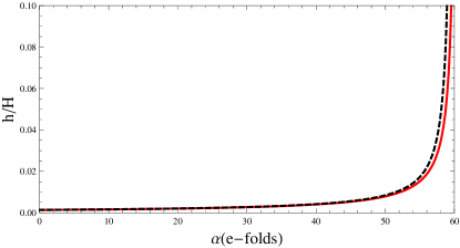
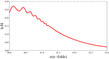
Figure 1: The left panel shows the evolution of anisotropy during inflation and the right panel after inflation (during when the scalar field is oscillating). Hα˙𝐻˙𝛼H\equiv\dot{\alpha} and hσ˙˙𝜎h\equiv\dot{\sigma}. The black dashed curve represents the approximate slow-roll solution during inflation and the straight red curves the numerical solution.

Refer to caption Refer to caption

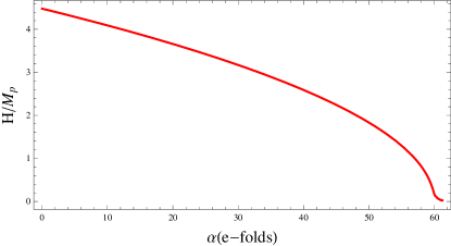
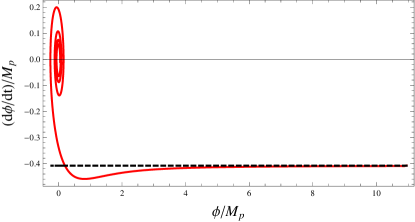
Figure 2: The left panel shows the evolution of the average Hubble rate (Hα˙𝐻˙𝛼H\equiv\dot{\alpha}) and the right panel is the phase plot of the scalar field. Again, the black dashed lines are the slow-roll solutions. Time is measured in units of m𝑚m.

We show in Figs. 12 the numerical evolution of the system. Note that the slow-roll and the numerical solutions are in good agreement with each other. The anisotropy in the single field model is increasing towards the end of inflation and decreases after inflation (as can be seen in the right panel of Fig. 1) during when the scalar field has an effective equation of state of matter. We are however interested in cases where the anisotropic expansion takes place at the onset of inflation (for example as in gcp ; gcp2 ; uzan1 ; uzan2 and soda1 ). The main reason is because we only want the largest observable scales to be modified from the perturbations that left the horizon during the anisotropic initial stage. This in turn might have some relevance to the alignment of the lowest multipoles. In the current case, all observable scales are modified (indeed smaller scales are modified even more since the anisotropy increases towards the end of inflation) and this is not compatible with observations. A simple possibility to overcome this difficulty is to introduce extra scalar fields as in the starting action (1). We discuss the background evolution for the simplest possibility of a two-field modification of the original proposal of Watanabe:2009ct in the next subsection.

II.2 Two Scalar Field Inflationary Background

In this section we discuss the simplest multi-field case of the action (1) with a=1𝑎1a=1. In this model, the extra scalar field ϕ1subscriptitalic-ϕ1\phi_{1} is not coupled to the vector field, and it is only relevant for the overall isotropic expansion of the universe. For the rest of the paper we will assume that V(ϕ)=m2ϕ2/2𝑉italic-ϕsuperscript𝑚2superscriptitalic-ϕ22V(\phi)=m^{2}\,\phi^{2}/2 and V1(ϕ1)=m12ϕ12/2subscript𝑉1subscriptitalic-ϕ1superscriptsubscript𝑚12superscriptsubscriptitalic-ϕ122V_{1}(\phi_{1})=m_{1}^{2}\,\phi_{1}^{2}/2. The ratio of the masses μm1/m𝜇subscript𝑚1𝑚\mu\equiv m_{1}/m is chosen to be smaller than 1. This choice leads to a two stage inflationary expansion. The first stage is driven mainly by ϕitalic-ϕ\phi, and due to its coupling with the vector field, this stage is anisotropic and it proceeds in a similar fashion as in the previous subsection. At the end of the first stage, the field ϕ1subscriptitalic-ϕ1\phi_{1} takes over the expansion, while the field ϕitalic-ϕ\phi starts oscillating. Since the expansion of the universe still proceeds, the Hubble friction will drive the field ϕitalic-ϕ\phi to zero and consequently, the coupling f(ϕ)𝑓italic-ϕf(\phi) approaches unity. Therefore, from (6), we clearly see that the effect of the vector field quickly diminishes. Thus, after the first stage, the universe quickly isotropizes and inflation proceeds isotropically until the field ϕ1subscriptitalic-ϕ1\phi_{1} starts oscillating. Problems related to an inflationary stage that has increasing anisotropy will be eliminated by the two stage modification.

As we have done in the previous section, we first study the solutions to the background evolution equations, which are given in this case as

3α˙23σ˙2=1Mp2[12ϕ˙2+12ϕ˙12+12m2ϕ2+12μ2m2ϕ12]+p~A22Mp2f2(ϕ)3superscript˙𝛼23superscript˙𝜎21superscriptsubscript𝑀𝑝2delimited-[]12superscript˙italic-ϕ212superscriptsubscript˙italic-ϕ1212superscript𝑚2superscriptitalic-ϕ212superscript𝜇2superscript𝑚2superscriptsubscriptitalic-ϕ12superscriptsubscript~𝑝𝐴22superscriptsubscript𝑀𝑝2superscript𝑓2italic-ϕ\displaystyle 3\dot{\alpha}^{2}-3\dot{\sigma}^{2}=\frac{1}{M_{p}^{2}}\,\left[\frac{1}{2}\,\dot{\phi}^{2}+\frac{1}{2}\,\dot{\phi}_{1}^{2}+\frac{1}{2}\,m^{2}\,\phi^{2}+\frac{1}{2}\,\mu^{2}\,m^{2}\,\phi_{1}^{2}\right]+\frac{\tilde{p}_{A}^{2}}{2M_{p}^{2}\,f^{2}(\phi)}
2α¨+3α˙2+3σ˙2=1Mp2[12ϕ˙212ϕ˙12+12m2ϕ2+12μ2m2ϕ12]p~A26Mp2f2(ϕ)2¨𝛼3superscript˙𝛼23superscript˙𝜎21superscriptsubscript𝑀𝑝2delimited-[]12superscript˙italic-ϕ212superscriptsubscript˙italic-ϕ1212superscript𝑚2superscriptitalic-ϕ212superscript𝜇2superscript𝑚2superscriptsubscriptitalic-ϕ12superscriptsubscript~𝑝𝐴26superscriptsubscript𝑀𝑝2superscript𝑓2italic-ϕ\displaystyle 2\ddot{\alpha}+3\dot{\alpha}^{2}+3\dot{\sigma}^{2}=\frac{1}{M_{p}^{2}}\,\left[-\frac{1}{2}\,\dot{\phi}^{2}-\frac{1}{2}\,\dot{\phi}_{1}^{2}+\frac{1}{2}\,m^{2}\,\phi^{2}+\frac{1}{2}\,\mu^{2}\,m^{2}\,\phi_{1}^{2}\right]-\frac{\tilde{p}_{A}^{2}}{6M_{p}^{2}\,f^{2}(\phi)}
σ¨+3α˙σ˙=p~A23Mp2f2(ϕ)¨𝜎3˙𝛼˙𝜎superscriptsubscript~𝑝𝐴23superscriptsubscript𝑀𝑝2superscript𝑓2italic-ϕ\displaystyle\ddot{\sigma}+3\dot{\alpha}\,\dot{\sigma}=\frac{\tilde{p}_{A}^{2}}{3M_{p}^{2}\,f^{2}(\phi)}
ϕ¨+3α˙ϕ˙+m2ϕp~A2f3(ϕ)f(ϕ)=0¨italic-ϕ3˙𝛼˙italic-ϕsuperscript𝑚2italic-ϕsuperscriptsubscript~𝑝𝐴2superscript𝑓3italic-ϕsuperscript𝑓italic-ϕ0\displaystyle\ddot{\phi}+3\dot{\alpha}\,\dot{\phi}+m^{2}\,\phi-\frac{\tilde{p}_{A}^{2}}{f^{3}(\phi)}\,f^{\prime}(\phi)=0
ϕ¨1+3α˙ϕ˙1+m2μ2ϕ12=0subscript¨italic-ϕ13˙𝛼subscript˙italic-ϕ1superscript𝑚2superscript𝜇2superscriptsubscriptitalic-ϕ120\displaystyle\ddot{\phi}_{1}+3\dot{\alpha}\,\dot{\phi}_{1}+m^{2}\,\mu^{2}\,\phi_{1}^{2}=0 (24)

where f(ϕ)=ecϕ2/2Mp2𝑓italic-ϕsuperscript𝑒𝑐superscriptitalic-ϕ22superscriptsubscript𝑀𝑝2f(\phi)=e^{c\,\phi^{2}/2M_{p}^{2}} as before. We can obtain slow-roll solutions similar to (19), in the first stage which proceeds anisotropically. Equations (16) are now modified to become

α˙2m26Mp2(ϕ2+μ2ϕ12),    3α˙ϕ˙m2ϕ+cp~A2Mp2ϕecϕ2/Mp2,    3α˙ϕ˙1m2μ2ϕ1formulae-sequencesuperscript˙𝛼2superscript𝑚26superscriptsubscript𝑀𝑝2superscriptitalic-ϕ2superscript𝜇2superscriptsubscriptitalic-ϕ12formulae-sequence3˙𝛼˙italic-ϕsuperscript𝑚2italic-ϕ𝑐superscriptsubscript~𝑝𝐴2superscriptsubscript𝑀𝑝2italic-ϕsuperscript𝑒𝑐superscriptitalic-ϕ2superscriptsubscript𝑀𝑝23˙𝛼subscript˙italic-ϕ1superscript𝑚2superscript𝜇2subscriptitalic-ϕ1\dot{\alpha}^{2}\approx\frac{m^{2}}{6M_{p}^{2}}\,\left(\phi^{2}+\mu^{2}\,\phi_{1}^{2}\right)\,\,\,\,,\,\,\,\,3\,\dot{\alpha}\,\dot{\phi}\approx-m^{2}\,\phi+\frac{c\,\tilde{p}_{A}^{2}}{M_{p}^{2}}\,\phi\,e^{-c\,\phi^{2}/M_{p}^{2}}\,\,\,\,,\,\,\,\,3\,\dot{\alpha}\,\dot{\phi}_{1}\approx-m^{2}\,\mu^{2}\,\phi_{1} (25)

Initially, the field ϕitalic-ϕ\phi drives the expansion, so ϕ2μ2ϕ12much-greater-thansuperscriptitalic-ϕ2superscript𝜇2superscriptsubscriptitalic-ϕ12\phi^{2}\gg\mu^{2}\,\phi_{1}^{2}, and the slow roll solutions for the first stage is simply given similar to (19) as

ecϕ2/Mp2c2p~A2m2Mp2(c1)ϕ˙23mMpcsuperscript𝑒𝑐superscriptitalic-ϕ2superscriptsubscript𝑀𝑝2superscript𝑐2superscriptsubscript~𝑝𝐴2superscript𝑚2superscriptsubscript𝑀𝑝2𝑐1˙italic-ϕ23𝑚subscript𝑀𝑝𝑐\displaystyle e^{c\,\phi^{2}/M_{p}^{2}}\approx\frac{c^{2}\,\tilde{p}_{A}^{2}}{m^{2}\,M_{p}^{2}\,(c-1)}\,\,\,\rightarrow\,\,\,\dot{\phi}\approx-\sqrt{\frac{2}{3}}\,\frac{m\,M_{p}}{c}
ϕ˙123mMpμ2ϕϕ1subscript˙italic-ϕ123𝑚subscript𝑀𝑝superscript𝜇2italic-ϕsubscriptitalic-ϕ1\displaystyle\dot{\phi}_{1}\approx-\sqrt{\frac{2}{3}}\,\frac{m\,M_{p}\,\mu^{2}}{\phi}\,\phi_{1} (26)

and the anisotropy is given precisely as in equation (21). After this first stage ends, the isotropic expansion of the universe is driven by ϕ1subscriptitalic-ϕ1\phi_{1} and this second stage is described by the following slow-roll solution

ϕ˙123mMpμsubscript˙italic-ϕ123𝑚subscript𝑀𝑝𝜇\dot{\phi}_{1}\approx-\sqrt{\frac{2}{3}}\,m\,M_{p}\,\mu (27)

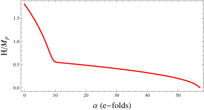
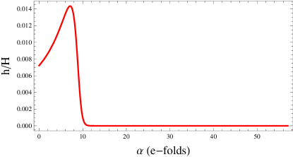
We also integrate the system (24) numerically and the results are shown in Figs 34. As we have done in the previous section, we use the slow-roll solutions and the constraint equation (the first of (24)) to determine the initial conditions ϕ˙in,ϕ˙1in,σ˙in,α˙insubscript˙italic-ϕ𝑖𝑛subscript˙italic-ϕ1𝑖𝑛subscript˙𝜎𝑖𝑛subscript˙𝛼𝑖𝑛\dot{\phi}_{in},\,\dot{\phi}_{1in},\,\dot{\sigma}_{in},\,\dot{\alpha}_{in} 555In order to find the approximate slow-roll solutions, one has to ignore the effect of the second field ϕ1subscriptitalic-ϕ1\phi_{1} initially. Although this approximation is fairly accurate, we let the numerical evolution to run for a few e-folds until the real attractor solution is reached.. The initial conditions for the scale factors are set as αin=0subscript𝛼𝑖𝑛0\alpha_{in}=0 and σinsubscript𝜎𝑖𝑛\sigma_{in} chosen to satisfy σ(tend)=0𝜎subscript𝑡𝑒𝑛𝑑0\sigma(t_{end})=0 at the end of inflation. We have chosen ϕin=5Mpsubscriptitalic-ϕ𝑖𝑛5subscript𝑀𝑝\phi_{in}=5M_{p}, ϕ1in=14Mpsubscriptitalic-ϕ1𝑖𝑛14subscript𝑀𝑝\phi_{1in}=14M_{p} and μ=1/10𝜇110\mu=1/10, which gives around 606060 e-folds of inflation, with the first 101010 e-folds being anisotropic.

Refer to caption Refer to caption

Figure 3: The left panel shows the evolution of the average Hubble expansion. The right panel shows the evolution of anisotropy, where Hα˙𝐻˙𝛼H\equiv\dot{\alpha} and hσ˙˙𝜎h\equiv\dot{\sigma}.

Refer to caption

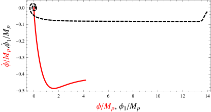
Figure 4: The phase portrait for the two scalar fields. The straight red line represents ϕitalic-ϕ\phi and the dashed black line represents ϕ1subscriptitalic-ϕ1\phi_{1}. Time is measured in units of m𝑚m.

In this type of background, when the anisotropic expansion takes place at the onset of inflation, we expect that only the largest scale perturbations are improved and at small scales standard results are recovered.

III Perturbations

This section is devoted to the study of the perturbations around the anisotropic inflationary background solutions we have discussed in the previous section. We will first discuss the decomposition of perturbations around the background configuration, which is different from standard scalar-vector-tensor decomposition used for isotropic backgrounds. The isotropic background solutions have a 3 dimensional rotational and translational symmetry for constant time slices, therefore small fluctuations are decomposed using the representations of the SO(3)𝑆𝑂3SO(3) group. In such a decomposition, one identifies decoupled classes of fluctuations and according to their transformation properties, one can identify scalar, vector (transverse) and tensor modes(transverse-traceless). Such a decomposition can still be considered in an anisotropic background, however fluctuations classified as scalar, vector and tensor would be coupled in the linearized calculation 666We refer to both the computation of the quadratic action and linearized Einstein equations as the ”linearized calculation”, since the latter follows from the previous. (see for example uzan1 ; uzan2 ). Instead, we make use of the left over 2 dimensional rotational symmetry of the yz𝑦𝑧y-z plane of the Bianchi-I metric (2) in order to decompose small fluctuations around the background as in gcp2 ; hcp2 . In such a two dimensional decomposition, there are two decoupled sets of perturbations, the 2d2𝑑2d scalar and 2d2𝑑2d vector modes. We will compute the quadratic action of the small fluctuations for both type of modes and study them separately. Since the universe isotropizes either after inflation in the single field model, or after the first stage of anisotropy in the double field model, the observables today are best defined if we use standard isotropic definitions of fluctuations. Therefore, we will also find the map between the 2d2𝑑2d decomposition and the standard 3d3𝑑3d isotropic decomposition, using which we will determine the power spectra for the gravitational wave polarizations {h×,h+}subscriptsubscript\{h_{\times},\,h_{+}\} and the curvature perturbation {\cal R} today (which are defined with respect to an isotropic background). This procedure is described in detail in the appendix.

III.1 Decomposition of Perturbations

We decompose the perturbations of the metric and the vector field by exploiting the 2d2𝑑2d isotropy of the background as

δgμν𝛿subscript𝑔𝜇𝜈\displaystyle\delta g_{\mu\nu} =\displaystyle= (2Φa1χb(iB+Bi)2a2Ψab1(iB~+B~i)b2(2Σδij2ijEiEjjEi))2Φ𝑎subscript1𝜒𝑏subscript𝑖𝐵subscript𝐵𝑖missing-subexpression2superscript𝑎2Ψ𝑎𝑏subscript1subscript𝑖~𝐵subscript~𝐵𝑖missing-subexpressionmissing-subexpressionsuperscript𝑏22Σsubscript𝛿𝑖𝑗2subscript𝑖subscript𝑗𝐸subscript𝑖subscript𝐸𝑗subscript𝑗subscript𝐸𝑖\displaystyle\left(\begin{array}[]{ccc}-2\Phi&a\,\partial_{1}\,\chi&b\left(\partial_{i}\,B+B_{i}\right)\\ &-2\,a^{2}\,\Psi&a\,b\,\partial_{1}\,\left(\partial_{i}\,\tilde{B}+\tilde{B}_{i}\right)\\ &&b^{2}\,\left(-2\Sigma\,\delta_{ij}-2\,\partial_{i}\,\partial_{j}\,E-\partial_{i}\,E_{j}-\partial_{j}\,E_{i}\right)\end{array}\right) (31)
δAμ𝛿subscript𝐴𝜇\displaystyle\delta A_{\mu} =\displaystyle= (α0,α1,iα+αi)subscript𝛼0subscript𝛼1subscript𝑖𝛼subscript𝛼𝑖\displaystyle\left(\alpha_{0},\,\alpha_{1},\,\partial_{i}\alpha+\alpha_{i}\right) (32)

Additionally, the system of perturbations contain the fluctuations of the scalar field(s) δϕa𝛿subscriptitalic-ϕ𝑎\delta\phi_{a}. Indices i,j=2,3formulae-sequence𝑖𝑗23i,j=2,3 span the isotropic 2d2𝑑2d-plane. The perturbations {δϕa,Φ,χ,B,Ψ,B~,Σ,E,α0,α1,α}𝛿subscriptitalic-ϕ𝑎Φ𝜒𝐵Ψ~𝐵Σ𝐸subscript𝛼0subscript𝛼1𝛼\{\delta\phi_{a},\,\Phi,\,\chi,\,B,\,\Psi,\,\tilde{B},\,\Sigma,\,E,\,\alpha_{0},\,\alpha_{1},\,\alpha\} are 2d2𝑑2d scalar perturbations, comprising one degree of freedom (d.o.f) each, and {Bi,B~i,Ei,αi}subscript𝐵𝑖subscript~𝐵𝑖subscript𝐸𝑖subscript𝛼𝑖\{B_{i},\,\tilde{B}_{i},\,E_{i},\,\alpha_{i}\} are 2d2𝑑2d vector modes which satisfy the transversality condition (iBi==0)subscript𝑖subscript𝐵𝑖0(\partial_{i}\,B_{i}=\dots=0). Therefore, the 2d2𝑑2d vector perturbations also comprise one d.o.f. each. The 2d2𝑑2d vector and scalar modes are decoupled at the linearized level.

We will work in the momentum space where a generic Fourier transformed mode is defined as

δ(x)=1(2π)3d3kδ(k)eikLxikT2yikT3z𝛿𝑥1superscript2𝜋3superscript𝑑3𝑘𝛿𝑘superscript𝑒𝑖subscript𝑘𝐿𝑥𝑖subscript𝑘𝑇2𝑦𝑖subscript𝑘𝑇3𝑧\delta\left(x\right)=\frac{1}{\left(2\pi\right)^{3}}\,\int\,d^{3}k\,\delta\left(k\right)\,e^{-i\,k_{L}\,x-i\,k_{T2}\,y-i\,k_{T3}\,z} (33)

We can use the residual 2d2𝑑2d-isotropy to fix the comoving momentum to be aligned in the xy𝑥𝑦x-y plane without any loss of generality. Namely, we set kT3=0subscript𝑘𝑇30k_{T3}=0 and kT=kT2subscript𝑘𝑇subscript𝑘𝑇2k_{T}=k_{T2} in what follows. Therefore, in Fourier space, the generic 2d2𝑑2d decomposition can be written as (before fixing the gauge)

δgμν(k)𝛿subscript𝑔𝜇𝜈𝑘\displaystyle\delta g_{\mu\nu}\,(k) =\displaystyle= (2ΨiakLχibkTBbB32a2ΨabkLkTB~iabkLB~3b2(2Σ+2kT2E)ib2kTE32b2Σ)2Ψ𝑖𝑎subscript𝑘𝐿𝜒𝑖𝑏subscript𝑘𝑇𝐵𝑏subscript𝐵3missing-subexpression2superscript𝑎2Ψ𝑎𝑏subscript𝑘𝐿subscript𝑘𝑇~𝐵𝑖𝑎𝑏subscript𝑘𝐿subscript~𝐵3missing-subexpressionmissing-subexpressionsuperscript𝑏22Σ2superscriptsubscript𝑘𝑇2𝐸𝑖superscript𝑏2subscript𝑘𝑇subscript𝐸3missing-subexpressionmissing-subexpressionmissing-subexpression2superscript𝑏2Σ\displaystyle\left(\begin{array}[]{cccc}-2\,\Psi&-i\,a\,k_{L}\,\chi&-i\,b\,k_{T}\,B&b\,B_{3}\\ &-2\,a^{2}\,\Psi&-a\,b\,k_{L}\,k_{T}\,\tilde{B}&-i\,a\,b\,k_{L}\,\tilde{B}_{3}\\ &&b^{2}\,\left(-2\,\Sigma+2k_{T}^{2}\,E\right)&i\,b^{2}\,k_{T}\,E_{3}\\ &&&-2\,b^{2}\,\Sigma\end{array}\right) (38)
δAμ(k)𝛿subscript𝐴𝜇𝑘\displaystyle\delta A_{\mu}(k) =\displaystyle= (α0,α1,ikTα,α3)subscript𝛼0subscript𝛼1𝑖subscript𝑘𝑇𝛼subscript𝛼3\displaystyle\left(\alpha_{0},\,\alpha_{1},\,-i\,k_{T}\,\alpha,\,\alpha_{3}\right) (39)

Notice that, for the 2d2𝑑2d vector modes, fixing kT=kT2subscript𝑘𝑇subscript𝑘𝑇2k_{T}=k_{T2} resulted in B2=B~2=E2=α2=0subscript𝐵2subscript~𝐵2subscript𝐸2subscript𝛼20B_{2}=\tilde{B}_{2}=E_{2}=\alpha_{2}=0. Under the infinitesimal coordinate transformation xμxμ+ϵμsuperscript𝑥𝜇superscript𝑥𝜇superscriptitalic-ϵ𝜇x^{\mu}\rightarrow x^{\mu}+\epsilon^{\mu}, the metric perturbations transform as

δgμνδgμνgμν,σ(0)ϵσgμσ(0)ϵ,νσgσν(0)ϵ,μσ\delta g_{\mu\nu}\rightarrow\delta g_{\mu\nu}-g_{\mu\nu,\sigma}^{(0)}\,\epsilon^{\sigma}-g_{\mu\sigma}^{(0)}\,\epsilon^{\sigma}_{,\nu}-g_{\sigma\nu}^{(0)}\,\epsilon^{\sigma}_{,\mu} (40)

where we have decomposed

ϵμ(k)=(ξ0,ikLξ1,ikTξ,ξ3)superscriptitalic-ϵ𝜇𝑘superscript𝜉0𝑖subscript𝑘𝐿superscript𝜉1𝑖subscript𝑘𝑇𝜉superscript𝜉3\epsilon^{\mu}(k)=\left(\xi^{0},\,-i\,k_{L}\,\xi^{1},\,-i\,k_{T}\,\xi,\,\xi^{3}\right) (41)

We choose to fix the coordinate gauge freedom by setting B~=Σ=E=E3=0~𝐵Σ𝐸subscript𝐸30\tilde{B}=\Sigma=E=E_{3}=0, namely we solve for the infinitesimal transformation to satisfy

ξ0=1HbΣ,ξ=E,ξ1=ba(B~+baE),ξ3=E3formulae-sequencesuperscript𝜉01subscript𝐻𝑏Σformulae-sequence𝜉𝐸formulae-sequencesuperscript𝜉1𝑏𝑎~𝐵𝑏𝑎𝐸superscript𝜉3subscript𝐸3\displaystyle\xi^{0}=-\frac{1}{H_{b}}\,\Sigma\,\,\,\,,\,\,\,\,\xi=-E\,\,\,\,,\,\,\,\,\xi^{1}=\frac{b}{a}\,\left(\tilde{B}+\frac{b}{a}\,E\right)\,\,\,\,,\,\,\,\,\xi^{3}=-E_{3} (42)

Since the action is invariant under the U(1)𝑈1U(1) gauge transformation, we can exploit this symmetry to eliminate one of the vector field perturbations. Namely, using the invariance δAμδAμ+μλ𝛿subscript𝐴𝜇𝛿subscript𝐴𝜇subscript𝜇𝜆\delta A_{\mu}\rightarrow\delta A_{\mu}+\partial_{\mu}\,\lambda, we set α=0𝛼0\alpha=0 in (32). This choice completely fixes the U(1)𝑈1U(1) gauge freedom. In summary, the complete system of perturbations, after fixing the coordinate and U(1)𝑈1U(1) gauge freedoms, contain three 2d2𝑑2d vector modes {B~3,α3,B3}subscript~𝐵3subscript𝛼3subscript𝐵3\{\tilde{B}_{3},\,\alpha_{3},\,B_{3}\} and six 2d2𝑑2d scalar modes {Φ,χ,B,Ψ,α0,α1}Φ𝜒𝐵Ψsubscript𝛼0subscript𝛼1\{\Phi,\,\chi,\,B,\,\Psi,\,\alpha_{0},\,\alpha_{1}\}. We will also have additional scalar modes coming from the fluctuations of the scalar field(s) δϕa𝛿subscriptitalic-ϕ𝑎\delta\phi_{a}. We will show in the following section that, not all the perturbations are dynamical, namely some perturbations enter into the quadratic action without any time derivatives. Such modes are lagrange multipliers and they can be integrated out from the action adm . The modes {B~3,α3,Ψ,α1}subscript~𝐵3subscript𝛼3Ψsubscript𝛼1\{\tilde{B}_{3},\,\alpha_{3},\,\Psi,\,\alpha_{1}\} and perturbations of the scalar fields are dynamical modes. On the other hand, {B3,Φ,χ,B,α0}subscript𝐵3Φ𝜒𝐵subscript𝛼0\{B_{3},\,\Phi,\,\chi,\,B,\,\alpha_{0}\} are nondynamical modes as we will demonstrate.

As we have mentioned earlier, it is useful to find the connection between the perturbations defined with respect to the 2d2𝑑2d decomposition and perturbations defined with respect to standard isotropic decompositions. This is useful in discussing the phenomenological consequences. After the universe isotropizes, perturbations evolve in the standard way, what is different is that their solutions are nonstandard. However, it is useful to give results in terms of the modes which are commonly used in FRW studies. For definiteness, we find the transformation between our choice of the gauge given in equation (42) and the standard longitudinal gauge. Here we present the results and leave the details to the appendix. The perturbations in the 2d2𝑑2d decomposition are related to the perturbations of the longitudinal gauge as

B~3subscript~𝐵3\displaystyle\tilde{B}_{3} =\displaystyle= ikkL(kT2+b/akL2kT)h×𝑖𝑘subscript𝑘𝐿superscriptsubscript𝑘𝑇2𝑏𝑎superscriptsubscript𝑘𝐿2subscript𝑘𝑇subscript\displaystyle\frac{i}{k\,k_{L}}\,\left(\frac{k_{T}^{2}+b/a\,k_{L}^{2}}{k_{T}}\right)\,h_{\times}
ΨΨ\displaystyle\Psi =\displaystyle= (1HaHb)ψ{Ha2Hb+1k2[12kT2+b3a3kL2(1+ba2kL2+kT22kT2)]}h+1subscript𝐻𝑎subscript𝐻𝑏𝜓subscript𝐻𝑎2subscript𝐻𝑏1superscript𝑘2delimited-[]12superscriptsubscript𝑘𝑇2superscript𝑏3superscript𝑎3superscriptsubscript𝑘𝐿21𝑏𝑎2superscriptsubscript𝑘𝐿2superscriptsubscript𝑘𝑇22superscriptsubscript𝑘𝑇2subscript\displaystyle\left(1-\frac{H_{a}}{H_{b}}\right)\,\psi-\left\{\frac{H_{a}}{2H_{b}}+\frac{1}{k^{2}}\,\left[\frac{1}{2}\,k_{T}^{2}+\frac{b^{3}}{a^{3}}\,k_{L}^{2}\,\left(1+\frac{b}{a}\,\frac{2k_{L}^{2}+k_{T}^{2}}{2k_{T}^{2}}\right)\,\right]\,\right\}\,h_{+}
δϕ𝛿italic-ϕ\displaystyle\delta\phi =\displaystyle= δϕL+ϕ˙Hb(ψ+12h+).𝛿superscriptitalic-ϕ𝐿˙italic-ϕsubscript𝐻𝑏𝜓12subscript\displaystyle\delta\phi^{L}+\frac{\dot{\phi}}{H_{b}}\,\left(\psi+\frac{1}{2}\,h_{+}\right). (43)

In the above equations, the terms in the left hand side are perturbations defined with respect to the 2d2𝑑2d decomposition and the terms in the right hand side are perturbations in the longitudinal gauge, where h×,h+subscriptsubscripth_{\times},\,h_{+} are the two gravitational wave polarizations, ψ𝜓\psi is the spatial scalar perturbation and δϕL𝛿superscriptitalic-ϕ𝐿\delta\phi^{L} is the scalar field perturbation (any generic scalar field in the model). These relations are useful in computing the power spectra of the gravitational waves and curvature perturbation.

III.2 General Properties of Coupled System of Perturbations

In this subsection, we discuss the general properties of the coupled system of perturbations that arise in this study. Our main discussion is based on the quadratic action for perturbations, which we need in order to determine initial conditions by canonical quantization. We compute the action for perturbations in quadratic order by inserting the decompositions (32), ϕ=ϕ0+δϕitalic-ϕsubscriptitalic-ϕ0𝛿italic-ϕ\phi=\phi_{0}+\delta\phi and ϕa=ϕa0+δϕasubscriptitalic-ϕ𝑎subscriptitalic-ϕ𝑎0𝛿subscriptitalic-ϕ𝑎\phi_{a}=\phi_{a0}+\delta\phi_{a} into (1), after fixing the U(1)𝑈1U(1) and coordinate gauges as described in the previous subsection. We note that the 2d2𝑑2d scalar and 2d2𝑑2d vector perturbations decouple in the quadratic action. We will provide explicit expressions for the scalar and vector actions in the following sections. Next we integrate out the nondynamical modes from the action, to obtain an action in terms of the dynamical modes only. More specifically, we extremize the quadratic action with respect to the nondynamical modes and obtain equations of motions for them (which are actually constraint equations). Then we solve for the nondynamical modes from their equations of motion, and insert the solutions back into the starting action. The final action we obtain depends only on the dynamical modes. The next step we perform is to find linear combinations of modes that canonically normalize the quadratic action. More specifically, the quadratic action after integrating out the nondynamical modes is formally of the type S𝑑td3k(δ˙iKijδ˙j+δ˙iΛijδjδiΩij2δj)similar-to𝑆differential-d𝑡superscript𝑑3𝑘subscript˙𝛿𝑖subscript𝐾𝑖𝑗subscript˙𝛿𝑗subscript˙𝛿𝑖subscriptΛ𝑖𝑗subscript𝛿𝑗subscript𝛿𝑖subscriptsuperscriptΩ2𝑖𝑗subscript𝛿𝑗S\sim\int dt\,d^{3}k\,(\dot{\delta}_{i}\,K_{ij}\,\dot{\delta}_{j}+\dot{\delta}_{i}\,\Lambda_{ij}\,\delta_{j}-\delta_{i}\,\Omega^{2}_{ij}\,\delta_{j}), where δisubscript𝛿𝑖\delta_{i} denotes the dynamical modes. We find linear combinations δi=Rijδcjsubscript𝛿𝑖subscript𝑅𝑖𝑗subscript𝛿𝑐𝑗\delta_{i}=R_{ij}\,\delta_{cj} such that δ˙iKijδ˙j=12δ˙ciδ˙ci+subscript˙𝛿𝑖subscript𝐾𝑖𝑗subscript˙𝛿𝑗12subscript˙𝛿𝑐𝑖subscript˙𝛿𝑐𝑖\dot{\delta}_{i}\,K_{ij}\,\dot{\delta}_{j}=\frac{1}{2}\,\dot{\delta}_{ci}\,\dot{\delta}_{ci}+\ldots where the dots denote mixed terms. The modes δcisubscript𝛿𝑐𝑖\delta_{ci} are the canonical modes. At the moment we will study a generic action obtained after canonically normalizing the starting action, which will be relevant for both 2d2𝑑2d vector and scalar modes. This action reads

Scan=12dtd3k{𝚽˙𝚽˙+(i𝚽˙𝐗𝚽+h.c.)p2𝚽(𝟏+ω2p2)𝚽}S_{can}=\frac{1}{2}\,\int\,dt\,d^{3}k\,\left\{\dot{\bf\Phi}^{{\dagger}}\,\dot{\bf\Phi}+\left(i\,\dot{\bf\Phi}^{{\dagger}}\,{\bf X}\,{\bf\Phi}+{\rm h.c.}\right)-p^{2}\,{\bf\Phi}^{{\dagger}}\,\left({\bf 1}+\frac{\omega^{2}}{p^{2}}\right)\,{\bf\Phi}\right\} (44)

where 𝚽𝚽{\bf\Phi} is a column vector made from the canonically normalized perturbations, 𝐗𝐗{\bf X} is a symmetric matrix and ω2superscript𝜔2{\bf\omega}^{2} is a hermitian matrix. In the above action, p𝑝p is the physical momentum with p2=pL2+pT2superscript𝑝2superscriptsubscript𝑝𝐿2superscriptsubscript𝑝𝑇2p^{2}=p_{L}^{2}+p_{T}^{2} where pL=kL/asubscript𝑝𝐿subscript𝑘𝐿𝑎p_{L}=k_{L}/a and pT=kT/bsubscript𝑝𝑇subscript𝑘𝑇𝑏p_{T}=k_{T}/b. We would like to perform a unitary transformation in the field space in order to get rid of the mixed terms 𝚽˙X𝚽superscript˙𝚽𝑋𝚽{\dot{\bf\Phi}}^{{\dagger}}\,X\,{\bf\Phi} and reduce the action to a canonical form that can be used to quantize the fields (and in turn obtain the initial conditions). This can be achieved by a unitary matrix 𝐔𝐔{\bf U} so that 𝚽=𝐔𝚿𝚽𝐔𝚿{\bf\Phi}={\bf U}\,{\bf\Psi} (The mixed terms can also be eliminated in the level of the Hamiltonian by canonical transformations. See for example Grisa:2009yy ). We choose the matrix 𝐔𝐔{\bf U} to satisfy

𝐔˙+i𝐗𝐔=0.˙𝐔𝑖𝐗𝐔0{\dot{\bf U}}+i\,{\bf X}\,{\bf U}=0. (45)

Inserting the transformation back into (44) and using (45) (with the unitarity condition on 𝐔𝐔{\bf U}), we get

S=12𝑑td3k[𝚿˙𝚿˙𝚿𝐔(p2+ω2+𝐗𝐗)𝐔𝚿].𝑆12differential-d𝑡superscript𝑑3𝑘delimited-[]superscript˙𝚿˙𝚿superscript𝚿superscript𝐔superscript𝑝2superscript𝜔2superscript𝐗𝐗𝐔𝚿S=\frac{1}{2}\,\int\,dt\,d^{3}k\,\left[\dot{\bf\Psi}^{{\dagger}}\,\dot{\bf\Psi}-{\bf\Psi}^{{\dagger}}\,{\bf U}^{{\dagger}}\,\left(p^{2}+\omega^{2}+{\bf X}^{{\dagger}}\,{\bf X}\right)\,{\bf U}\,{\bf\Psi}\right]. (46)

We will show in the following sections that the matrix 𝐗𝐗{\bf X} is of the order of the average Hubble scale H𝐻H (i.e. 𝐗=O(H)𝐗O𝐻{\bf X}={\rm O}(H)) and the matrix ω2superscript𝜔2\omega^{2} is of the order of Hubble scale squared (i.e. ω2=O(H2)superscript𝜔2Osuperscript𝐻2\omega^{2}={\rm O}(H^{2})). This means that in the deep UV/subhorizon regime, where pHmuch-greater-than𝑝𝐻p\gg H, these matrices will become negligible compared to p2superscript𝑝2p^{2}. Therefore, for modes that are deep inside the horizon initially, the above action reduces to a form which has diagonal mass terms

S=12𝑑td3k[𝚿˙𝚿˙p2𝚿𝚿+O(H2)]𝑆12differential-d𝑡superscript𝑑3𝑘delimited-[]superscript˙𝚿˙𝚿superscript𝑝2superscript𝚿𝚿Osuperscript𝐻2S=\frac{1}{2}\,\int\,dt\,d^{3}k\,\left[\dot{\bf\Psi}^{{\dagger}}\,\dot{\bf\Psi}-p^{2}\,{\bf\Psi}^{{\dagger}}\,{\bf\Psi}+{\rm O}(H^{2})\right] (47)

In this limit when the mass terms are diagonal, the mode expansion for field 𝚿𝚿{\bf\Psi} simply reads

𝚿^(x)=d3k(2π)3/2[eikxv(t)a^(k)+eikxv(t)a^(k)]^𝚿𝑥superscript𝑑3𝑘superscript2𝜋32delimited-[]superscript𝑒𝑖𝑘𝑥𝑣𝑡^𝑎𝑘superscript𝑒𝑖𝑘𝑥superscript𝑣𝑡superscript^𝑎𝑘\hat{\bf\Psi}(x)=\int\,\frac{d^{3}k}{\left(2\pi\right)^{3/2}}\,\left[e^{i\,\overrightarrow{k}\cdot\overrightarrow{x}}\,v(t)\,\hat{a}(k)+e^{-i\,\overrightarrow{k}\cdot\overrightarrow{x}}\,v^{*}(t)\,\hat{a}^{{\dagger}}(k)\right] (48)

The creation and annihilation operators a^(k),a^(k)^𝑎𝑘superscript^𝑎𝑘\hat{a}(k),\,\hat{a}^{{\dagger}}(k) obey the standard bosonic commutation relations and the mode functions v(t)𝑣𝑡v(t) satisfy

v¨+p2v=0.¨𝑣superscript𝑝2𝑣0\ddot{v}+p^{2}\,v=0. (49)

The above equation can be solved using the WKB approximation in the adiabatic limit, which gives

v(t)=12ωeiω𝑑t𝑣𝑡12𝜔superscript𝑒𝑖𝜔differential-dsuperscript𝑡v(t)=\frac{1}{\sqrt{2\omega}}\,e^{-i\,\int\,\omega\,dt^{\prime}} (50)

where ω𝜔\omega is given by

ω𝜔\displaystyle\omega =\displaystyle= pp¨4p2+38p˙2p3+𝑝¨𝑝4superscript𝑝238superscript˙𝑝2superscript𝑝3\displaystyle p-\frac{\ddot{p}}{4p^{2}}+\frac{3}{8}\,\frac{\dot{p}^{2}}{p^{3}}+\dots (51)
=\displaystyle= p+O(H2)𝑝𝑂superscript𝐻2\displaystyle p+O(H^{2})

In the above equation, \dots represent higher order corrections which are suppressed by higher powers of H𝐻H in the adiabatic solution. This is also consistent with the accuracy of the mode expansion (48). It is of course possible to neglect the mixed terms proportional to 𝐗𝐗{\bf X} and ω2superscript𝜔2\omega^{2} from the beginning. In this way the action for the original fields 𝚽𝚽{\bf\Phi} is canonical, however we would be working with an accuracy O(Hin/pin)Osubscript𝐻𝑖𝑛subscript𝑝𝑖𝑛{\rm O}(H_{in}/p_{in}) rather than O(Hin2/pin2)Osuperscriptsubscript𝐻𝑖𝑛2superscriptsubscript𝑝𝑖𝑛2{\rm O}(H_{in}^{2}/p_{in}^{2}). This situation is more difficult in terms of the numerical computation needed, since to achieve the desired accuracy, one has to start the numerical evolution much deeper inside the horizon. Moreover, initial conditions in the standard isotropic case are also given to an accuracy of O(Hin/pin)2Osuperscriptsubscript𝐻𝑖𝑛subscript𝑝𝑖𝑛2{\rm O}(H_{in}/p_{in})^{2}, therefore we choose to perform the field rotation to eliminate the 𝐗O(H)similar-to𝐗O𝐻{\bf X}\sim{\rm O}(H) terms and work with the fields 𝚿𝚿{\bf\Psi}. The field rotation can be performed trivially for the case of 2d2𝑑2d vector perturbations. The case for the 2d2𝑑2d scalar modes are more subtle, therefore we leave the discussion of scalar modes to a separate publication.

The canonical quantization procedure outlined above determines the adiabatic initial conditions for the modes 𝚿𝚿{\bf\Psi}. We are however interested in the values of the entries of 𝚽𝚽{\bf\Phi} evaluated at the end of inflation, which are related to the primordial power spectra. We will show in the next section that the matrix 𝐗𝐗{\bf X} along with the off-diagonal entries of ω2superscript𝜔2\omega^{2} is proportional to the anisotropy, so they vanish before the end of inflation in the two field model. Therefore, it is possible to choose the transformation matrix 𝐔𝐔{\bf U} that satisfies 𝐔(tend)=𝟏𝐔subscript𝑡𝑒𝑛𝑑1{\bf U}(t_{end})={\bf 1}, which in turn implies that 𝐔(ω2+𝐗𝐗)𝐔superscript𝐔superscript𝜔2superscript𝐗𝐗𝐔{\bf U}^{{\dagger}}\,\left(\omega^{2}+{\bf X}^{{\dagger}}\,{\bf X}\right)\,{\bf U} is also diagonal at tendsubscript𝑡𝑒𝑛𝑑t_{end} (tendsubscript𝑡𝑒𝑛𝑑t_{end} is the time when inflation ends). Then we have 𝚽(tend)=𝚿(tend)𝚽subscript𝑡𝑒𝑛𝑑𝚿subscript𝑡𝑒𝑛𝑑{\bf\Phi}(t_{end})={\bf\Psi}(t_{end}) and we use the following equality to compute the two point functions for the starting modes 𝚽𝚽{\bf\Phi};

<ΨaΨb>|tend=<ΦaΦb>|tendevaluated-atexpectationsuperscriptsubscriptΨ𝑎subscriptΨ𝑏subscript𝑡𝑒𝑛𝑑evaluated-atexpectationsuperscriptsubscriptΦ𝑎subscriptΦ𝑏subscript𝑡𝑒𝑛𝑑<\Psi_{a}^{{\dagger}}\,\Psi_{b}>|_{t_{end}}=<\Phi_{a}^{{\dagger}}\,\Phi_{b}>|_{t_{end}} (52)

for the components of the fields. Therefore, instead of working with the original fields 𝚽𝚽{\bf\Phi} we work with the transformed fields 𝚿𝚿{\bf\Psi}. Notice that passing to the fields 𝚿𝚿{\bf\Psi} was an important step, since the action is in its canonical form with diagonal mass terms p2superscript𝑝2p^{2} (up to accuracy O(H2)Osuperscript𝐻2{\rm O}(H^{2})) in the deep UV regime. Therefore, this field can be quantized and p𝑝p represents the energy of the each particle created by a^(k)superscript^𝑎𝑘\hat{a}^{{\dagger}}(k). The quantization procedure also determines the mode functions v𝑣v, which in turn determines initial conditions for the perturbations.

In the next subsection, we will discuss the evolution of the 2d2𝑑2d vector modes, which will be related to the power spectrum of the gravitational wave polarization h×subscripth_{\times}.

III.3 2d Vector Perturbations

We now discuss the 2d2𝑑2d vector perturbations of the two field inflationary background solution discussed in the previous section. As we have argued earlier, the quadratic action for the 2d2𝑑2d vector and scalar modes decouple, so we concentrate on the vector piece here. The action for the 2d2𝑑2d vector perturbations in momentum space, up to a total time derivative, is calculated as

S2dVsubscript𝑆2𝑑𝑉\displaystyle S_{2dV} =\displaystyle= Mp24𝑑td3ke3α2σ2dVsuperscriptsubscript𝑀𝑝24differential-d𝑡superscript𝑑3𝑘superscript𝑒3𝛼2𝜎subscript2𝑑𝑉\displaystyle\frac{M_{p}^{2}}{4}\,\int\,dt\,d^{3}k\,e^{3\alpha-2\sigma}\,{\cal L}_{2dV}
2dVsubscript2𝑑𝑉\displaystyle{\cal L}_{2dV} =\displaystyle= e2α2σpL2|B~˙3|2+2e2αf2(ϕ)Mp2|α˙3|2eαpL2(B~˙3B3+h.c.)+2eσp~ApLMp2(iα˙3B~3+h.c.)\displaystyle e^{2\alpha-2\sigma}\,p_{L}^{2}\,\left|\dot{\tilde{B}}_{3}\right|^{2}+2\,e^{-2\alpha}\,\frac{f^{2}(\phi)}{M_{p}^{2}}\,\left|\dot{\alpha}_{3}\right|^{2}-e^{\alpha}\,p_{L}^{2}\,\left(\dot{\tilde{B}}_{3}^{*}\,B_{3}+{\rm h.c.}\right)+2\,e^{-\sigma}\,\frac{\tilde{p}_{A}\,p_{L}}{M_{p}^{2}}\,\left(i\,\dot{\alpha}_{3}^{*}\,\tilde{B}_{3}+{\rm h.c.}\right) (53)
e2α2σpL2(pT29σ˙2p~A2Mp2f2(ϕ))|B~3|2+3eασ˙pL2(B~3B3+h.c.)\displaystyle-e^{2\alpha-2\sigma}\,p_{L}^{2}\,\left(p_{T}^{2}-9\dot{\sigma}^{2}-\frac{\tilde{p}_{A}^{2}}{M_{p}^{2}\,f^{2}(\phi)}\right)\,\left|\tilde{B}_{3}\right|^{2}+3\,e^{\alpha}\,\dot{\sigma}\,p_{L}^{2}\,\left(\tilde{B}_{3}^{*}\,B_{3}+{\rm h.c.}\right)
2e2αp2Mp2f2(ϕ)|α3|2+2eα+σp~ApLMp2(iα3B3+h.c.)+e2σp2|B3|2\displaystyle-2e^{-2\alpha}\,\frac{p^{2}}{M_{p}^{2}}\,f^{2}(\phi)\,\left|\alpha_{3}\right|^{2}+2\,e^{-\alpha+\sigma}\,\frac{\tilde{p}_{A}\,p_{L}}{M_{p}^{2}}\,\left(i\,\alpha_{3}^{*}\,B_{3}+{\rm h.c.}\right)+e^{2\sigma}\,p^{2}\,\left|B_{3}\right|^{2}

where we have used the physical momenta pLkL/asubscript𝑝𝐿subscript𝑘𝐿𝑎p_{L}\equiv k_{L}/a, pT=kT/bsubscript𝑝𝑇subscript𝑘𝑇𝑏p_{T}=k_{T}/b and p=pL2+pT2𝑝superscriptsubscript𝑝𝐿2superscriptsubscript𝑝𝑇2p=\sqrt{p_{L}^{2}+p_{T}^{2}}. As can be seen from (53), the mode B3subscript𝐵3B_{3} is nondynamical, so it can be integrated out from the action by solving its equation of motion. The solution for B3subscript𝐵3B_{3} is obtained as

B3=eα2σ[2ipLp~AMp2p2e2α+σα3+pL2p2(B~˙33σ˙B~3)]subscript𝐵3superscript𝑒𝛼2𝜎delimited-[]2𝑖subscript𝑝𝐿subscript~𝑝𝐴superscriptsubscript𝑀𝑝2superscript𝑝2superscript𝑒2𝛼𝜎subscript𝛼3superscriptsubscript𝑝𝐿2superscript𝑝2subscript˙~𝐵33˙𝜎subscript~𝐵3B_{3}=e^{\alpha-2\sigma}\,\left[\frac{2\,i\,p_{L}\,\tilde{p}_{A}}{M_{p}^{2}\,p^{2}}\,e^{-2\alpha+\sigma}\,\alpha_{3}+\frac{p_{L}^{2}}{p^{2}}\,\left(\dot{\tilde{B}}_{3}-3\,\dot{\sigma}\,\tilde{B}_{3}\right)\right] (54)

We insert the solution (54) back into the action (53) and up to a total time derivative, we obtain

S2dVsubscript𝑆2𝑑𝑉\displaystyle S_{2dV} =\displaystyle= 12dtd3k{|H˙×|2+|Δ˙|2+p~ApT2Mppf(ϕ)(iH˙×Δ+iH×Δ˙+h.c.)\displaystyle\frac{1}{2}\,\int\,dt\,d^{3}k\,\Bigg{\{}|\dot{H}_{\times}|^{2}+|\dot{\Delta}_{-}|^{2}+\frac{\tilde{p}_{A}\,p_{T}}{\sqrt{2}\,M_{p}\,p\,f(\phi)}\,\left(i\,\dot{H}_{\times}^{*}\,\Delta_{-}+i\,H_{\times}\,\dot{\Delta}_{-}^{*}+{\rm h.c.}\right) (59)
(H×Δ)(Ω112Ω122Ω122Ω222)(H×Δ)}\displaystyle\qquad\qquad\qquad\qquad-\left(H_{\times}^{*}\,\,\,\,\Delta_{-}^{*}\right)\,\left(\begin{array}[]{cc}\Omega_{11}^{2}&\Omega_{12}^{2}\\ \Omega_{12}^{*2}&\Omega_{22}^{2}\end{array}\right)\,\left(\begin{array}[]{c}H_{\times}\\ \Delta_{-}\end{array}\right)\Bigg{\}}

where the canonical modes H×subscript𝐻H_{\times} and ΔsubscriptΔ\Delta_{-} are related to the starting modes as

B~3=2ppLpTMpe52α+2σH×,α3=eα/2+σf(ϕ)Δformulae-sequencesubscript~𝐵32𝑝subscript𝑝𝐿subscript𝑝𝑇subscript𝑀𝑝superscript𝑒52𝛼2𝜎subscript𝐻subscript𝛼3superscript𝑒𝛼2𝜎𝑓italic-ϕsubscriptΔ\tilde{B}_{3}=\frac{\sqrt{2}\,p}{p_{L}\,p_{T}\,M_{p}}\,e^{-\frac{5}{2}\,\alpha+2\sigma}\,H_{\times}\,\,\,\,,\,\,\,\,\alpha_{3}=\frac{e^{-\alpha/2+\sigma}}{f(\phi)}\,\Delta_{-} (60)

and the mass terms Ω2superscriptΩ2\Omega^{2} are defined as

Ω112superscriptsubscriptΩ112\displaystyle\Omega_{11}^{2} \displaystyle\equiv p294α˙2+34Mp2(ϕ˙2+ϕ˙12)+92(pL4p4+6pL2pT2p4pT4p4)σ˙2+p~A22Mp2f2(ϕ)(pL4p4pT4p4)superscript𝑝294superscript˙𝛼234superscriptsubscript𝑀𝑝2superscript˙italic-ϕ2superscriptsubscript˙italic-ϕ1292superscriptsubscript𝑝𝐿4superscript𝑝46superscriptsubscript𝑝𝐿2superscriptsubscript𝑝𝑇2superscript𝑝4superscriptsubscript𝑝𝑇4superscript𝑝4superscript˙𝜎2superscriptsubscript~𝑝𝐴22superscriptsubscript𝑀𝑝2superscript𝑓2italic-ϕsuperscriptsubscript𝑝𝐿4superscript𝑝4superscriptsubscript𝑝𝑇4superscript𝑝4\displaystyle p^{2}-\frac{9}{4}\,\dot{\alpha}^{2}+\frac{3}{4M_{p}^{2}}\,\left(\dot{\phi}^{2}+\dot{\phi}_{1}^{2}\right)+\frac{9}{2}\,\left(\frac{p_{L}^{4}}{p^{4}}+6\frac{p_{L}^{2}\,p_{T}^{2}}{p^{4}}-\frac{p_{T}^{4}}{p^{4}}\right)\,\dot{\sigma}^{2}+\frac{\tilde{p}_{A}^{2}}{2M_{p}^{2}\,f^{2}(\phi)}\,\left(\frac{p_{L}^{4}}{p^{4}}-\frac{p_{T}^{4}}{p^{4}}\right)
Ω122superscriptsubscriptΩ122\displaystyle\Omega_{12}^{2} \displaystyle\equiv iω¯122=ip~ApT2Mppf(ϕ)(4pT25pL2p2σ˙+α˙f(ϕ)f(ϕ)ϕ˙)𝑖superscriptsubscript¯𝜔122𝑖subscript~𝑝𝐴subscript𝑝𝑇2subscript𝑀𝑝𝑝𝑓italic-ϕ4superscriptsubscript𝑝𝑇25superscriptsubscript𝑝𝐿2superscript𝑝2˙𝜎˙𝛼superscript𝑓italic-ϕ𝑓italic-ϕ˙italic-ϕ\displaystyle i\,{\bar{\omega}}_{12}^{2}=\frac{i\,\tilde{p}_{A}\,p_{T}}{\sqrt{2}\,M_{p}\,p\,f(\phi)}\,\left(\frac{4p_{T}^{2}-5p_{L}^{2}}{p^{2}}\,\dot{\sigma}+\dot{\alpha}-\frac{f^{\prime}(\phi)}{f(\phi)}\,\dot{\phi}\right)
Ω222superscriptsubscriptΩ222\displaystyle\Omega_{22}^{2} =\displaystyle= p214α˙2+14Mp2(ϕ˙2+ϕ˙12)2α˙σ˙+12σ˙2+p~A22Mp2f2(ϕ)5pL2+pT2p2p~A2f2(ϕ)f(ϕ)2f2(ϕ)superscript𝑝214superscript˙𝛼214superscriptsubscript𝑀𝑝2superscript˙italic-ϕ2superscriptsubscript˙italic-ϕ122˙𝛼˙𝜎12superscript˙𝜎2superscriptsubscript~𝑝𝐴22superscriptsubscript𝑀𝑝2superscript𝑓2italic-ϕ5superscriptsubscript𝑝𝐿2superscriptsubscript𝑝𝑇2superscript𝑝2superscriptsubscript~𝑝𝐴2superscript𝑓2italic-ϕsuperscript𝑓superscriptitalic-ϕ2superscript𝑓2italic-ϕ\displaystyle p^{2}-\frac{1}{4}\,\dot{\alpha}^{2}+\frac{1}{4M_{p}^{2}}\,\left(\dot{\phi}^{2}+\dot{\phi}_{1}^{2}\right)-2\,\dot{\alpha}\,\dot{\sigma}+\frac{1}{2}\,\dot{\sigma}^{2}+\frac{\tilde{p}_{A}^{2}}{2M_{p}^{2}\,f^{2}(\phi)}\,\frac{5p_{L}^{2}+p_{T}^{2}}{p^{2}}-\frac{\tilde{p}_{A}^{2}}{f^{2}(\phi)}\,\frac{f^{\prime}(\phi)^{2}}{f^{2}(\phi)} (61)
+[2(α˙+σ˙)ϕ˙+V(ϕ)]f(ϕ)f(ϕ)f′′(ϕ)f(ϕ)ϕ˙2delimited-[]2˙𝛼˙𝜎˙italic-ϕsuperscript𝑉italic-ϕsuperscript𝑓italic-ϕ𝑓italic-ϕsuperscript𝑓′′italic-ϕ𝑓italic-ϕsuperscript˙italic-ϕ2\displaystyle+\left[2\left(\dot{\alpha}+\dot{\sigma}\right)\,\dot{\phi}+V^{\prime}(\phi)\right]\,\frac{f^{\prime}(\phi)}{f(\phi)}-\frac{f^{\prime\prime}(\phi)}{f(\phi)}\,\dot{\phi}^{2}

The action (59) has regular kinetic terms, and therefore there is no ghost instability in the 2d2𝑑2d vector sector, as expected. Note that the matrix 𝐗𝐗{\bf X} along with the mass matrix terms Ω2superscriptΩ2\Omega^{2} satisfy

Ω122=O(H2),Ω112=Ω222=p2+O(H2),formulae-sequencesuperscriptsubscriptΩ122Osuperscript𝐻2superscriptsubscriptΩ112superscriptsubscriptΩ222superscript𝑝2Osuperscript𝐻2\displaystyle\Omega_{12}^{2}={\rm O}\left(H^{2}\right)\,\,\,\,,\,\,\,\Omega_{11}^{2}=\Omega_{22}^{2}=p^{2}+{\rm O}\left(H^{2}\right)\,\,\,,
p~AMpf(ϕ)=6α˙26σ˙22Mp2(V(ϕ)+V1(ϕ1))1Mp2(ϕ˙2+ϕ˙12)O(H)subscript~𝑝𝐴subscript𝑀𝑝𝑓italic-ϕ6superscript˙𝛼26superscript˙𝜎22superscriptsubscript𝑀𝑝2𝑉italic-ϕsubscript𝑉1subscriptitalic-ϕ11superscriptsubscript𝑀𝑝2superscript˙italic-ϕ2superscriptsubscript˙italic-ϕ12similar-toO𝐻\displaystyle\frac{\tilde{p}_{A}}{M_{p}\,f(\phi)}=\sqrt{6\dot{\alpha}^{2}-6\dot{\sigma}^{2}-\frac{2}{M_{p}^{2}}\,\left(V(\phi)+V_{1}(\phi_{1})\right)-\frac{1}{M_{p}^{2}}\,\left(\dot{\phi}^{2}+\dot{\phi}_{1}^{2}\right)}\sim{\rm O}(H) (62)

therefore, the action (59) is formally of the type given in (44) with 𝚽𝚽{\bf\Phi} and matrix 𝐗𝐗{\bf X} given by

𝚽(H×Δ),𝐗(0λλ0),λp~ApT2Mpf(ϕ)pformulae-sequence𝚽subscript𝐻subscriptΔformulae-sequence𝐗0𝜆𝜆0𝜆subscript~𝑝𝐴subscript𝑝𝑇2subscript𝑀𝑝𝑓italic-ϕ𝑝{\bf\Phi}\equiv\left(\begin{array}[]{c}H_{\times}\\ \Delta_{-}\end{array}\right)\,\,\,\,,\,\,\,\,{\bf X}\equiv\left(\begin{array}[]{cc}0&\lambda\\ \lambda&0\end{array}\right)\,\,\,\,\,,\,\,\,\,\,\,\lambda\equiv\frac{\tilde{p}_{A}\,p_{T}}{\sqrt{2}\,M_{p}\,f(\phi)\,p} (63)

We can therefore determine the transformation matrix 𝐔𝐔{\bf U}, that eliminates the mixed terms 𝚽˙𝐗𝚽superscript˙𝚽𝐗𝚽\dot{\bf\Phi}^{{\dagger}}\,{\bf X}\,{\bf\Phi} by solving 𝐔˙+i𝐗𝐔=0˙𝐔𝑖𝐗𝐔0\dot{\bf U}+i\,{\bf X}\,{\bf U}=0, which can be solved by diagonalizing the matrix 𝐗𝐗{\bf X}. Notice that 𝐑𝐗𝐑=DXsuperscript𝐑𝐗𝐑subscript𝐷𝑋{\bf R}^{{\dagger}}\,{\bf X}\,{\bf R}=D_{X} where

𝐑=12(1111),DX=(λ00λ)formulae-sequence𝐑121111subscript𝐷𝑋𝜆00𝜆{\bf R}=\frac{1}{\sqrt{2}}\,\left(\begin{array}[]{cc}1&-1\\ 1&1\end{array}\right)\,\,\,\,,\,\,\,\,D_{X}=\left(\begin{array}[]{cc}\lambda&0\\ 0&-\lambda\end{array}\right) (64)

Therefore (45) is solved by

𝐔=𝐑eitDX𝑑t𝐖0𝐔𝐑superscript𝑒𝑖superscript𝑡subscript𝐷𝑋differential-dsuperscript𝑡subscript𝐖0{\bf U}={\bf R}\,e^{-i\,\int^{t}\,D_{X}\,dt^{\prime}}\,{\bf W}_{0} (65)

where 𝐖0subscript𝐖0{\bf W}_{0} is a constant unitary matrix, which does not have any physical relevance. Therefore, we choose 𝐖0=𝐑subscript𝐖0superscript𝐑{\bf W}_{0}={\bf R}^{{\dagger}}, so that 𝐔=𝟏𝐔1{\bf U}={\bf 1} when λ=0𝜆0\lambda=0 (i.e. when anisotropy vanishes). We can now determine the new mass matrix for the transformed fields 𝚿𝚿{\bf\Psi}, which are given by

ΩΨ2=𝐔[Ω2+𝐗𝐗]𝐔superscriptsubscriptΩΨ2superscript𝐔delimited-[]superscriptΩ2superscript𝐗𝐗𝐔\Omega_{\Psi}^{2}={\bf U}^{{\dagger}}\,\left[\Omega^{2}+{\bf X}^{{\dagger}}\,{\bf X}\right]\,{\bf U} (66)

where the entries of ΩΨ2superscriptsubscriptΩΨ2\Omega_{\Psi}^{2} are explicitly given by

ΩΨ 112superscriptsubscriptΩΨ112\displaystyle\Omega_{\Psi\,11}^{2} =\displaystyle= λ2+Ω112+Ω2222+Ω112Ω2222cos[2(t)]+ω¯122sin[2(t)]superscript𝜆2superscriptsubscriptΩ112superscriptsubscriptΩ2222superscriptsubscriptΩ112superscriptsubscriptΩ22222𝑡superscriptsubscript¯𝜔1222𝑡\displaystyle\lambda^{2}+\frac{\Omega_{11}^{2}+\Omega_{22}^{2}}{2}+\frac{\Omega_{11}^{2}-\Omega_{22}^{2}}{2}\,\cos\left[2{\cal I}(t)\right]+{\bar{\omega}}_{12}^{2}\,\sin\left[2{\cal I}(t)\right]
ΩΨ 222superscriptsubscriptΩΨ222\displaystyle\Omega_{\Psi\,22}^{2} =\displaystyle= λ2+Ω112+Ω2222Ω112Ω2222cos[2(t)]ω¯122sin[2(t)]superscript𝜆2superscriptsubscriptΩ112superscriptsubscriptΩ2222superscriptsubscriptΩ112superscriptsubscriptΩ22222𝑡superscriptsubscript¯𝜔1222𝑡\displaystyle\lambda^{2}+\frac{\Omega_{11}^{2}+\Omega_{22}^{2}}{2}-\frac{\Omega_{11}^{2}-\Omega_{22}^{2}}{2}\,\cos\left[2{\cal I}(t)\right]-{\bar{\omega}}_{12}^{2}\,\sin\left[2{\cal I}(t)\right]
ΩΨ 122superscriptsubscriptΩΨ122\displaystyle\Omega_{\Psi\,12}^{2} =\displaystyle= ΩΨ 212=i{ω¯122cos[2(t)]Ω112Ω2222sin[2(t)]}superscriptsubscriptΩΨ212𝑖superscriptsubscript¯𝜔1222𝑡superscriptsubscriptΩ112superscriptsubscriptΩ22222𝑡\displaystyle-\Omega_{\Psi\,21}^{2}=i\,\left\{{\bar{\omega}}_{12}^{2}\,\cos\left[2{\cal I}(t)\right]-\frac{\Omega_{11}^{2}-\Omega_{22}^{2}}{2}\,\sin\left[2{\cal I}(t)\right]\right\} (67)

where

(t)tktλ(t)𝑑t={constantt>tisotktλ(t)𝑑tt<tiso𝑡superscriptsubscriptsubscript𝑡𝑘𝑡𝜆superscript𝑡differential-dsuperscript𝑡casesconstant𝑡subscript𝑡𝑖𝑠𝑜superscriptsubscriptsubscript𝑡𝑘𝑡𝜆superscript𝑡differential-dsuperscript𝑡𝑡subscript𝑡𝑖𝑠𝑜{\cal I}(t)\equiv\int_{t_{k}}^{t}\,\lambda(t^{\prime})\,dt^{\prime}=\Bigg{\{}\begin{array}[]{c}{\rm constant}\,\,\,\,\,\,\,\,\,\,t>t_{iso}\\ \int_{t_{k}}^{t}\,\lambda(t^{\prime})\,dt^{\prime}\,\,\,\,\,t<t_{iso}\end{array} (68)

Here, tisosubscript𝑡𝑖𝑠𝑜t_{iso} is the time when the universe isotropizes so λ(ttiso)=0𝜆𝑡subscript𝑡𝑖𝑠𝑜0\lambda(t\geq t_{iso})=0. The lower limit tksubscript𝑡𝑘t_{k} in the integral is chosen for each comoving momentum k𝑘k such that the constant value for t>tiso𝑡subscript𝑡𝑖𝑠𝑜t>t_{iso} is unity 777It is possible to keep the lower limit in the integral arbitrary, since it has no physical relevance. However, for an arbitrary value, the mass terms for the fields 𝚿𝚿{\bf\Psi} will in general be nondiagonal at the end of inflation. In this case, one has to further rotate the fields (by a constant matrix) to obtain the physical modes. We perform this step from the beginning by choosing tksubscript𝑡𝑘t_{k} corrrectly, so that 𝐔=1𝐔1{\bf U}=1 at the end of inflation.. This ensures that 𝐔(tiso)=𝐔(tend)=𝟏𝐔subscript𝑡𝑖𝑠𝑜𝐔subscript𝑡𝑒𝑛𝑑1{\bf U}(t_{iso})={\bf U}(t_{end})={\bf 1} since

𝐔(cos[(t)]isin[(t)]isin[(t)]cos[(t)])𝟏whenttiso𝐔𝑡𝑖𝑡𝑖𝑡𝑡1when𝑡subscript𝑡𝑖𝑠𝑜{\bf U}\equiv\left(\begin{array}[]{cc}\cos\left[{\cal I}(t)\right]&-i\sin\left[{\cal I}(t)\right]\\ -i\sin\left[{\cal I}(t)\right]&\cos\left[{\cal I}(t)\right]\end{array}\right)\rightarrow{\bf 1}\,\,\,\,\,{\rm when}\,\,\,\,\,t\geq t_{iso} (69)

Finally, the fields 𝚿𝚿{\bf\Psi} satisfy the evolution equations

Ψ¨a+ΩΨab2Ψb=0subscript¨Ψ𝑎superscriptsubscriptΩΨ𝑎𝑏2subscriptΨ𝑏0\ddot{\Psi}_{a}+\Omega_{\Psi\,ab}^{2}\,\Psi_{b}=0 (70)

with initial conditions on the entries of ΨasubscriptΨ𝑎\Psi_{a} set by the form of the mode function v(t)𝑣𝑡v(t) which are given deep inside the horizon as

ΨainsubscriptΨ𝑎𝑖𝑛\displaystyle\Psi_{a\,in} =\displaystyle= 12p+O(H2)12𝑝Osuperscript𝐻2\displaystyle\frac{1}{\sqrt{2p}}+{\rm O}(H^{2})
Ψ˙ainsubscript˙Ψ𝑎𝑖𝑛\displaystyle\dot{\Psi}_{a\,in} =\displaystyle= 12p(ipp˙2p)+O(H2)12𝑝𝑖𝑝˙𝑝2𝑝Osuperscript𝐻2\displaystyle\frac{1}{\sqrt{2p}}\,\left(-i\,p-\frac{\dot{p}}{2p}\right)+{\rm O}(H^{2}) (71)

up to a nonphysical phase.

In the next section, we will numerically evaluate the evolution equations (70) with adiabatic initial conditions (71) for a range of comoving momenta, and determine the two point functions <ΨaΨb>|tendevaluated-atexpectationsuperscriptsubscriptΨ𝑎subscriptΨ𝑏subscript𝑡𝑒𝑛𝑑<\Psi_{a}^{{\dagger}}\,\Psi_{b}>|_{t_{end}} which coincides with <ΦaΦb>|tendevaluated-atexpectationsuperscriptsubscriptΦ𝑎subscriptΦ𝑏subscript𝑡𝑒𝑛𝑑<\Phi_{a}^{{\dagger}}\,\Phi_{b}>|_{t_{end}} as we argued before. Finally, using (60) and (43) we deduce the power spectrum (which is related to the calculated two point functions) for the gravitational wave polarization h×subscripth_{\times}. We will provide the study of the 2d2𝑑2d scalar perturbations in the appendix and leave the study of the power spectrum for the scalar modes and the comparison with observations in a separate publication.

IV Power Spectrum

This section is devoted to the study of the power spectrum of the gravitational wave polarization h×subscripth_{\times}. We will use the results of the previous sections to compute the evolution of the fields ΨΨ\Psi using their equations of motion given in (70) with the elements of the mass matrices given in (67). We perform the integration for a range of co-moving momenta kLsubscript𝑘𝐿k_{L} and kTsubscript𝑘𝑇k_{T}, which we parameterize as

kL=ξk,kT=1ξ2k,kkL2+kT2,     0ξ1.k_{L}=\xi\,k\,\,\,\,\,,\,\,\,\,\,k_{T}=\sqrt{1-\xi^{2}}\,k\,\,\,\,\,\,,\,\,\,\,\,\,k\equiv\sqrt{k_{L}^{2}+k_{T}^{2}}\,\,\,\,\,\,,\,\,\,\,\,0\leq\xi\leq 1. (72)

Therefore, ξ𝜉\xi is the cosine of the angle between the comoving momentum and the longitudinal component kLsubscript𝑘𝐿k_{L}. For each comoving mometa labelled by the two numbers {k,ξ}𝑘𝜉\{k,\xi\}, initial conditions are given in equation (71). The initial time tinsubscript𝑡𝑖𝑛t_{in} is chosen to be the moment when

ka(tin)=50H(tin)ork=50α˙(tin)eα(tin)𝑘𝑎subscript𝑡𝑖𝑛50𝐻subscript𝑡𝑖𝑛or𝑘50˙𝛼subscript𝑡𝑖𝑛superscript𝑒𝛼subscript𝑡𝑖𝑛\frac{k}{a(t_{in})}=50\,H(t_{in})\,\,\,\,\,{\rm or}\,\,\,\,\,k=50\,\dot{\alpha}(t_{in})\,e^{\alpha(t_{in})} (73)

so that the physical momentum p𝑝p is sufficiently larger than the Hubble scale and the adiabatic initial conditions (71) are accurate. Since the mass matrix ΩΨ2superscriptsubscriptΩΨ2\Omega_{\Psi}^{2} depends on the background quantities, we integrate the equations (70) together with the background equations (24) with initial conditions and parameters m1,m2subscript𝑚1subscript𝑚2m_{1},\,m_{2} set as explained in subsection (II.2). Using (43) and (60) we can relate the gravitational wave polarization h×subscripth_{\times} to the canonical field H×subscript𝐻H_{\times} at the end of inflation (when σ=σ˙=0𝜎˙𝜎0\sigma=\dot{\sigma}=0, so a=b𝑎𝑏a=b)

h×=2iMpe32αH×.subscript2𝑖subscript𝑀𝑝superscript𝑒32𝛼subscript𝐻h_{\times}=\frac{\sqrt{2}}{i\,M_{p}}\,e^{-\frac{3}{2}\,\alpha}\,H_{\times}. (74)

We define the power spectrum for the gravitational wave mode h×subscripth_{\times} as

P×(k)(k3|h×|2)|t=tendsubscript𝑃𝑘evaluated-atsuperscript𝑘3superscriptsubscript2𝑡subscript𝑡𝑒𝑛𝑑P_{\times}(\overrightarrow{k})\equiv\left(k^{3}\,|h_{\times}|^{2}\right)|_{t=t_{end}} (75)

At the end of inflation, the fields ΨΨ\Psi is identical to the starting fields ΦΦ\Phi, so the power spectrum of the gravitational wave mode h×subscripth_{\times}is obtained by evaluating the correlation function <Ψ1Ψ1>=<Φ1Φ1>expectationsuperscriptsubscriptΨ1subscriptΨ1expectationsuperscriptsubscriptΦ1subscriptΦ1<\Psi_{1}^{*}\,\Psi_{1}>=<\Phi_{1}^{*}\,\Phi_{1}> and using (74) which gives

P×(k)=2k3Mp2e3α(tend)|Ψ1(tend)|2.subscript𝑃𝑘2superscript𝑘3superscriptsubscript𝑀𝑝2superscript𝑒3𝛼subscript𝑡𝑒𝑛𝑑superscriptsubscriptΨ1subscript𝑡𝑒𝑛𝑑2P_{\times}(\overrightarrow{k})=\frac{2k^{3}}{M_{p}^{2}}\,e^{-3\,\alpha(t_{end})}\,|\Psi_{1}(t_{end})|^{2}. (76)

In Figures 5,6 we show the power spectrum obtained from the numerical integration of the background and perturbation equations. In Fig 5 , parts of the power spectrum is shown for fixed values of ξ=0, 0.5, 1𝜉00.51\xi=0,\,0.5,\,1 and 101kisok103/2kisosuperscript101subscript𝑘𝑖𝑠𝑜𝑘superscript1032subscript𝑘𝑖𝑠𝑜10^{-1}\,k_{iso}\leq k\leq 10^{3/2}\,k_{iso}. We have define kisosubscript𝑘𝑖𝑠𝑜k_{iso} to be the value of the comoving momentum, when k=a(tiso)H(tiso)=α˙(tiso)eα(tiso)𝑘𝑎subscript𝑡𝑖𝑠𝑜𝐻subscript𝑡𝑖𝑠𝑜˙𝛼subscript𝑡𝑖𝑠𝑜superscript𝑒𝛼subscript𝑡𝑖𝑠𝑜k=a(t_{iso})\,H(t_{iso})=\dot{\alpha}(t_{iso})\,e^{\alpha(t_{iso})} where tisosubscript𝑡𝑖𝑠𝑜t_{iso} is the time of isotropization (we define it to be the time when h/H=103𝐻superscript103h/H=10^{-3} numerically). In Fig. 6, we show contour plot of the full spectrum P×(k)subscript𝑃𝑘P_{\times}(\overrightarrow{k}).

Refer to caption

Figure 5: Parts of the power spectrum for h×subscripth_{\times} are shown for ξ=0𝜉0\xi=0 (straight line), ξ=0.5𝜉0.5\xi=0.5 (dashed line) and ξ=1𝜉1\xi=1(dotted line).

Refer to caption

Figure 6: The contour plot of the full power spectrum P×(k)subscript𝑃𝑘P_{\times}(k).

At large scales for k>kiso𝑘subscript𝑘𝑖𝑠𝑜k>k_{iso}, there is more power and the spectrum has angular dependence. This in turn could be related to the CMB anomalies. Note that the spectrum reduces to the standard nearly scale invariant form when k>kiso𝑘subscript𝑘𝑖𝑠𝑜k>k_{iso}. Indeed, we have checked that for k>kiso𝑘subscript𝑘𝑖𝑠𝑜k>k_{iso}, the power spectrum reduces to

P×(k>kiso)=ATknT,nT2ϵ=ϕ˙12α˙2Mp2formulae-sequencesubscript𝑃𝑘subscript𝑘𝑖𝑠𝑜subscript𝐴𝑇superscript𝑘subscript𝑛𝑇subscript𝑛𝑇2italic-ϵsuperscriptsubscript˙italic-ϕ12superscript˙𝛼2superscriptsubscript𝑀𝑝2P_{\times}(k>k_{iso})=A_{T}\,k^{n_{T}}\,\,\,\,\,,\,\,\,\,n_{T}\equiv-2\,\epsilon=-\frac{\dot{\phi}_{1}^{2}}{\dot{\alpha}^{2}\,M_{p}^{2}} (77)

where ϵitalic-ϵ\epsilon is the standard slow-roll parameter for the field ϕ1subscriptitalic-ϕ1\phi_{1}. Indeed, the the spectrum can be written as

P×(k)={aT(kkiso)f(ξ,k)k<kisoaT(kkiso)nTk>kiso.subscript𝑃𝑘cases<subscript𝑎𝑇superscript𝑘subscript𝑘𝑖𝑠𝑜𝑓𝜉𝑘𝑘subscript𝑘𝑖𝑠𝑜>subscript𝑎𝑇superscript𝑘subscript𝑘𝑖𝑠𝑜subscript𝑛𝑇𝑘subscript𝑘𝑖𝑠𝑜P_{\times}(\overrightarrow{k})=\Bigg{\{}\begin{array}[]{c}a_{T}\,\left(\frac{k}{k_{iso}}\right)^{f(\xi,\,k)}\,\,\,\,\,\,k\mathrel{\raise 1.29167pt\hbox{$<$\kern-7.5pt\lower 4.30554pt\hbox{$\sim$}}}k_{iso}\\ a_{T}\,\left(\frac{k}{k_{iso}}\right)^{n_{T}}\,\,\,\,\,\,\,\,\,k\mathrel{\raise 1.29167pt\hbox{$>$\kern-7.5pt\lower 4.30554pt\hbox{$\sim$}}}k_{iso}\end{array}. (78)

The form of the function f(ξ,k)𝑓𝜉𝑘f(\xi,k) is unknown, but it is possible to consider a generic expansion of the form

Log10P×=Log10aT+(c1+d1ξn1)x+(c2+d2ξn2)x2+(c3+d3ξn3)x3+subscriptLog10subscript𝑃subscriptLog10subscript𝑎𝑇subscript𝑐1subscript𝑑1superscript𝜉subscript𝑛1𝑥subscript𝑐2subscript𝑑2superscript𝜉subscript𝑛2superscript𝑥2subscript𝑐3subscript𝑑3superscript𝜉subscript𝑛3superscript𝑥3\displaystyle{\rm Log}_{10}P_{\times}={\rm Log}_{10}a_{T}+\left(c_{1}+d_{1}\,\xi^{n_{1}}\right)\,x+\left(c_{2}+d_{2}\,\xi^{n_{2}}\right)\,x^{2}+\left(c_{3}+d_{3}\,\xi^{n_{3}}\right)\,x^{3}+\dots
xLog10(kkiso)𝑥subscriptLog10𝑘subscript𝑘𝑖𝑠𝑜\displaystyle x\equiv{\rm Log}_{10}\left(\frac{k}{k_{iso}}\right) (79)

We fix the unknown parameters Log10aTsubscriptLog10subscript𝑎𝑇{\rm Log}_{10}a_{T} (which coincides with the Log10aTsubscriptLog10subscript𝑎𝑇{\rm Log}_{10}a_{T} of the spectrum for k<kiso𝑘subscript𝑘𝑖𝑠𝑜k<k_{iso}) and c1,c2,c3subscript𝑐1subscript𝑐2subscript𝑐3c_{1},\,c_{2},\,c_{3} by fitting to the numerical spectrum when ξ=0𝜉0\xi=0. Then, we fix the parameters d1,d2,d3subscript𝑑1subscript𝑑2subscript𝑑3d_{1},\,d_{2},\,d_{3} by fitting to the numerical spectrum when ξ=1𝜉1\xi=1 (using the previous values of Log10aTsubscriptLog10subscript𝑎𝑇{\rm Log}_{10}a_{T} and c1,c2,c3subscript𝑐1subscript𝑐2subscript𝑐3c_{1},\,c_{2},\,c_{3}). Finally, we obtain the values of n1,n2,n3subscript𝑛1subscript𝑛2subscript𝑛3n_{1},\,n_{2},\,n_{3} by fitting to a spectrum at an intermediate value of ξ𝜉\xi. Increasing the number of terms in the expansion (79), increases the accuracy of the fit. For the spectra we have obtained above, the unknown parameters are obtained as

Log10aT0.43,c10.23,c20.83,c30.38formulae-sequencesimilar-to-or-equalssubscriptLog10subscript𝑎𝑇0.43formulae-sequencesimilar-to-or-equalssubscript𝑐10.23formulae-sequencesimilar-to-or-equalssubscript𝑐20.83similar-to-or-equalssubscript𝑐30.38\displaystyle{\rm Log}_{10}a_{T}\simeq-0.43,\,\,\,c_{1}\simeq-0.23,\,\,\,c_{2}\simeq 0.83,\,\,\,c_{3}\simeq 0.38
d10.82,d21.21,d30.69formulae-sequencesimilar-to-or-equalssubscript𝑑10.82formulae-sequencesimilar-to-or-equalssubscript𝑑21.21similar-to-or-equalssubscript𝑑30.69\displaystyle d_{1}\simeq 0.82,\,\,\,d_{2}\simeq 1.21,\,\,\,d_{3}\simeq 0.69
n13.94,n23.38,n33.34formulae-sequencesimilar-to-or-equalssubscript𝑛13.94formulae-sequencesimilar-to-or-equalssubscript𝑛23.38similar-to-or-equalssubscript𝑛33.34\displaystyle n_{1}\simeq 3.94,\,\,\,n_{2}\simeq 3.38,\,\,\,n_{3}\simeq 3.34 (80)

In Fig. 7, we show the fitted and numerical power spectra for k<kiso𝑘subscript𝑘𝑖𝑠𝑜k<k_{iso}, which are in good agreement. In Fig. 8, we show the numerical spectra for k>kiso𝑘subscript𝑘𝑖𝑠𝑜k>k_{iso}, which is of the standard nearly scale invariant form.
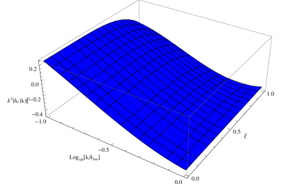
Refer to caption Refer to caption

Figure 7: The left panel shows the fitted spectrum using (79) and the right panel the numerical spectrum for k<kiso𝑘subscript𝑘𝑖𝑠𝑜k<k_{iso}. The fitted and numerical spectra are in good agreement.

.

Refer to caption

Figure 8: The power spectra at small scales for k>kiso𝑘subscript𝑘𝑖𝑠𝑜k>k_{iso}, which is of the standard nearly scale invariant form P×knTproportional-tosubscript𝑃superscript𝑘subscript𝑛𝑇P_{\times}\propto k^{n_{T}}.

The power spectrum for the gravitational wave mode h×subscripth_{\times} is not of the form P×=P×,iso(k)+δP×(k,ξ)subscript𝑃subscript𝑃𝑖𝑠𝑜𝑘𝛿subscript𝑃𝑘𝜉P_{\times}=P_{\times,\,iso}(k)+\delta P_{\times}(k,\xi) as one would naively expect for small anisotropy for k<kiso𝑘subscript𝑘𝑖𝑠𝑜k<k_{iso}, with |δP×||P×,iso|much-less-than𝛿subscript𝑃subscript𝑃𝑖𝑠𝑜|\delta P_{\times}|\ll|P_{\times,\,iso}|. This is due to the fact the the anisotropic background attractor is not continuously connected to standard isotropic solutions, i.e. there is no parameter with a certain limit which takes the anisotropic solution to the isotropic one. This is in contrast for example to the ACW model acw , where in the limit m20superscript𝑚20m^{2}\rightarrow 0 (m2superscript𝑚2m^{2} is the norm of the VEV of the vector field in the model), the background solution reduces to an isotropic limit. For the current case, attractors with c>1𝑐1c>1 (anisotropic) and c<1𝑐1c<1 (isotropic) are disconnected in the limit c1𝑐1c\rightarrow 1. Therefore, the behavior of the perturbations are dramatically different for k<kiso𝑘subscript𝑘𝑖𝑠𝑜k<k_{iso} and the spectrum is largely enhanced in this region (|δP×||P×,iso|much-less-than𝛿subscript𝑃subscript𝑃𝑖𝑠𝑜|\delta P_{\times}|\ll|P_{\times,\,iso}| is not satisfied). For phenomenological considerations, this result is not a desired one, since the CMB data would be consistent with a statistical anisotropy at large scales that would satisfy |δP×||P×,iso|much-less-than𝛿subscript𝑃subscript𝑃𝑖𝑠𝑜|\delta P_{\times}|\ll|P_{\times,\,iso}|. However, this model is the only vector field driven anisotropic inflationary model that does not suffer from any instability to our knowledge. Therefore, we believe that the results obtained in this section are still interesting.

V Conclusions

In this work we have considered anisotropic inflationary models with coupled vector and scalar fields. The coupling of the scalar field to the vector field is chosen to preserve the U(1)𝑈1U(1) gauge symmetry of the Lagrangian, therefore, the longitudinal polarization of the vector field, which has been shown to cause instabilities hcp1 ; hcp2 ; hcp3 , does not exist. The anisotropic expansion is achieved when the vector field has a VEV along one of the spatial directions. The anisotropic solution is an attractor, with anisotropy increasing towards the end of inflation, so these types of models are counter examples to the cosmic no hair conjecture Wald . We have considered a generalization of the original model introduced in reference Watanabe:2009ct , to include additional scalar fields, and specifically concentrated on the double scalar field case. This modification was done in order to achieve isotropization of the universe before the end of inflation. The original model with a single scalar field coupled to the vector field has an anisotropic inflationary background which persists until the end of inflation. In this type of background, perturbations at all scales are modified. In the two field modification, the extra field is not coupled to the vector field, and it is responsible for the overall isotropic expansion of the universe only. We have chosen the ratio of the masses of the scalar fields such that the inflationary expansion takes place in two steps, the first being anisotropic and the second is isotropic. Therefore, only the largest scale perturbations are modified and at small scales the standard spectrum is recovered. As we have discussed in the introduction, vector fields with a nonvanishing VEV have been introduced since isotropization takes place very quickly in a Bianchi-I background, (when anisotropy is only coming from initial conditions) and thus leads to a fine tuning. We have introduced a two phase inflation, with the second phase being isotropic. The transition to the second isotropic phase is indeed very quick, however the fine tuning has been relaxed compared to the previous case. The second isotropic phase should still be tuned to last around 606060 e-folds, but this tuning is not so strict, since it only affects the scale where the power spectrum becomes statistically isotropic. Previously, the tuning was more stringent, since inflation must last for 606060 e-folds in order that the largest scales are modified from the initial anisotropic conditions. A more important drawback of the inlfationary setup with only initial anisotropic conditions is that the initial singularity is very close to the time of isotropization, which is around one Hubble time. Thus, a calculation of the power spectrum shows that it becomes divergent at the largest scales gcp2  888This does not mean that the model is unstable, it reflects that nonlinear effects become important, and one has to go beyond linear perturbation theory..

We have studied the perturbations around the background configuration in detail, taking into account all the degrees of freedom of the system. Following the formalism developed in references gcp ; gcp2 , we have classified decoupled sets of perturbations around the anisotropic background and studied them separately. Furthermore, we have computed the quadratic action for perturbations and showed that the model is stable and consistent. We also found linear combinations of the perturbations which canonically normalize the action. This enabled us to quantize the system which in turn determined the initial conditions for the perturbations in the adiabatic vacuum. We then numerically integrated the equations of motion for the 2d2𝑑2d vector perturbations for a range of comoving momenta, which resulted in the power spectrum of the gravitational wave polarization h×subscripth_{\times}. We have only computed the quadratic action and determined the canonical modes for the 2d2𝑑2d scalar perturbations. We leave the study of the power spectra and the consequent phenomenology, which in turn is related to the curvature and h+subscripth_{+} gravitational wave spectrum, to a later publication.

The computed spectrum for h×subscripth_{\times} has certain interesting features, which might have some relevance to the observed CMB anomalies. First of all, the spectrum has angular dependence for k<kiso𝑘subscript𝑘𝑖𝑠𝑜k<k_{iso} which breaks the statistical isotropy at large scales, therefore leads to an alignment of the lowest multipoles as described in gcp ; gcp2 ; acw . Moreover, the spectrum reduces to the standard nearly scale invariant form for k>kiso𝑘subscript𝑘𝑖𝑠𝑜k>k_{iso}, so the higher multipoles are not affected from the vector field. We have shown that the power spectrum is formally of the form P×(k)=P×,iso(k)+δP×(k,ξ)subscript𝑃𝑘subscript𝑃𝑖𝑠𝑜𝑘𝛿subscript𝑃𝑘𝜉P_{\times}(\overrightarrow{k})=P_{\times,\,iso}(k)+\delta P_{\times}(k,\xi). We expect that this will be true also for the spectrum of scalar modes. We have also provided a functional form for δP×𝛿subscript𝑃\delta P_{\times} by fitting to the numerical spectrum in equation (79). Phenomenologically acceptable modifications to the large scale spectrum should satisfy |δP||Piso|much-less-than𝛿𝑃subscript𝑃𝑖𝑠𝑜|\delta P|\ll|P_{iso}|, however, we have shown that for the model under discussion, this is not the case. Although our results are obtained for the gravitational wave mode h×subscripth_{\times}, we expect a similar behavior also for the curvature spectrum, which can be compared with observations. At larger scales, the power spectrum is greatly enhanced satisfying |δP×|>|P×,iso|𝛿subscript𝑃subscript𝑃𝑖𝑠𝑜|\delta P_{\times}|>|P_{\times,\,iso}|. Although the anisotropy in the background is small (in the level of a percent, as can be seen from equation(21)), the modification to the spectrum at large scales is not small. This is due to the fact that the background attractor solution is disconnected from the standard isotropic solution and therefore, the behavior of perturbations are dramatically different. There is no parameter in the attractor solution that connects it continuously to the isotropic FRW limit. The anisotropy is always small and proportional to 1/c21superscript𝑐21/c^{2} and there is no finite limit in c𝑐c which can continuously deform the attractor solution to the isotropic solution. Therefore, the power spectrum cannot be approximated as to be the isotropic piece plus a small correction from anisotropy. This issue unfortunately limits the phenomenology of the model.

Even though the difficulties involved, anisotropic backgrounds still have potentially interesting phenomenological consequences. Off-diagonal correlations of the almsubscript𝑎𝑙𝑚a_{lm} coefficients of CMB temperature fluctuations arise in such backgrounds and can have relevance to the alignment of lowest multipoles. Moreover, at the largest scales, non standard scalar to tensor ratio is obtained, which can be tested by upcoming CMB experiments. The gravitational wave modes h+subscripth_{+} and h×subscripth_{\times} behave differently at large scales, therefore a future detection of gravitational waves might be tested against the consequences of an early stage of anisotropic inflation. In this paper, we have provided a solid example of anisotropic inflationary calculation of perturbations and computed the spectrum of h×subscripth_{\times} polarization of gravitational waves. Although the obtained spectrum has phenomenologically limited implications, we believe that our results are still relevant, since it is the first complete study of power spectrum in an anisotropic inflationary model driven by a vector field to our knowledge. In a further publication, we will study the spectrum of the curvature {\cal R} perturbation, which could then be compared with observational data.

Acknowledgements.
The author would like to thank Marco Peloso, Lorenzo Sorbo, Jose Cembranos for very useful discussions. This work is supported by the Graduate School at the University of Minnesota under the Doctoral Dissertation Fellowship.

VI Appendices

VI.1 Appendix I

In this appendix we derive the relations (43), which are used in the main text to compute the power spectrum of the gravitational wave mode h×subscripth_{\times}. These relations are also useful when the curvature and h+subscripth_{+} power spectra are calculated. For this calculation, one needs to analyze the 2d2𝑑2d scalar perturbations, which is done in the next appendix. We will study the power spectrum for the scalar modes in a separate publication.

We start with the decomposition of perturbations in the longitudinal gauge, when the universe is isotropic, which is given by

ds2=(1+2ϕ)dt2+2aVidtdxi+a2[(12ψ)δij+hij]dxidxj𝑑superscript𝑠212italic-ϕ𝑑superscript𝑡22𝑎subscript𝑉𝑖𝑑𝑡𝑑superscript𝑥𝑖superscript𝑎2delimited-[]12𝜓subscript𝛿𝑖𝑗subscript𝑖𝑗𝑑superscript𝑥𝑖𝑑superscript𝑥𝑗ds^{2}=-\left(1+2\phi\right)\,dt^{2}+2\,a\,V_{i}\,dt\,dx^{i}+a^{2}\,\left[\left(1-2\psi\right)\,\delta_{ij}+h_{ij}\right]\,dx^{i}\,dx^{j} (81)

where i=1,2,3𝑖123i=1,2,3. Visubscript𝑉𝑖V_{i}’s are vector modes satisfying iVi=0subscript𝑖subscript𝑉𝑖0\partial_{i}\,V_{i}=0 and hijsubscript𝑖𝑗h_{ij}’s are transverse-traceless modes satisfying ihij=hii=0subscript𝑖subscript𝑖𝑗subscript𝑖𝑖0\partial_{i}\,h_{ij}=h_{ii}=0. Since the spatial slices are isotropic, we can fix the comoving momentum to lie entirely along the x-direction k=(k, 0, 0)𝑘𝑘 0 0\overrightarrow{k}=\left(k,\,0,\,0\right), without any loss of generality. In this case, the longitudinal gauge can be expressed in Fourier space as

δgμν(k)=(2ϕ0V2V32a2ψ00a2(2ψ+h+)a2h×a2h×a2(2ψh+))𝛿subscript𝑔𝜇𝜈𝑘2italic-ϕ0subscript𝑉2subscript𝑉3missing-subexpression2superscript𝑎2𝜓00missing-subexpressionmissing-subexpressionsuperscript𝑎22𝜓subscriptsuperscript𝑎2subscriptmissing-subexpressionmissing-subexpressionsuperscript𝑎2subscriptsuperscript𝑎22𝜓subscript\delta g_{\mu\nu}(k)=\left(\begin{array}[]{cccc}-2\phi&0&V_{2}&V_{3}\\ &-2a^{2}\,\psi&0&0\\ &&a^{2}\,\left(-2\,\psi+h_{+}\right)&-a^{2}\,h_{\times}\\ &&-a^{2}\,h_{\times}&a^{2}\,\left(-2\,\psi-h_{+}\right)\end{array}\right) (82)

We can now rotate the momentum from the x-direction, to xy𝑥𝑦x-y plane in order to make the comparison with the 2d2𝑑2d decomposition. Namely, we perform the following rotation over the comoving momentum:

(kLkT)=1k(kLkTkTkL)(k0)subscript𝑘𝐿subscript𝑘𝑇1𝑘subscript𝑘𝐿subscript𝑘𝑇subscript𝑘𝑇subscript𝑘𝐿𝑘0\left(\begin{array}[]{c}k_{L}\\ k_{T}\end{array}\right)=\frac{1}{k}\,\left(\begin{array}[]{cc}k_{L}&-k_{T}\\ k_{T}&k_{L}\end{array}\right)\,\left(\begin{array}[]{c}k\\ 0\end{array}\right) (83)

where k=kL2+kT2𝑘superscriptsubscript𝑘𝐿2superscriptsubscript𝑘𝑇2k=\sqrt{k_{L}^{2}+k_{T}^{2}}. The matrix appearing in (83) also determines the Jacobian matrix which fixes the coordinate transformation rule from the metric with k=(k,0,0)𝑘𝑘00\overrightarrow{k}=(k,0,0) (82) to a metric with k=(kL,kT,0)𝑘subscript𝑘𝐿subscript𝑘𝑇0\overrightarrow{k}=(k_{L},k_{T},0). The resulting decomposition will determine the 2d2𝑑2d-decomposed longitudinal gauge. Using the appropriate scale factors a𝑎a and b𝑏b where necessary to take into account the anisotropy of the universe, the 2d2𝑑2d decomposed longitudinal gauge becomes

δgμνL(k)=(2ϕakTkV2bkLkV2bV3a2(2ψ+kT2k2h+)abkLkTk2h+abkTkh×b2(2ψ+kL2k2h+)b2kLkh×b2(2ψh+))𝛿superscriptsubscript𝑔𝜇𝜈𝐿𝑘2italic-ϕ𝑎subscript𝑘𝑇𝑘subscript𝑉2𝑏subscript𝑘𝐿𝑘subscript𝑉2𝑏subscript𝑉3missing-subexpressionsuperscript𝑎22𝜓superscriptsubscript𝑘𝑇2superscript𝑘2subscript𝑎𝑏subscript𝑘𝐿subscript𝑘𝑇superscript𝑘2subscript𝑎𝑏subscript𝑘𝑇𝑘subscriptmissing-subexpressionmissing-subexpressionsuperscript𝑏22𝜓superscriptsubscript𝑘𝐿2superscript𝑘2subscriptsuperscript𝑏2subscript𝑘𝐿𝑘subscriptmissing-subexpressionmissing-subexpressionmissing-subexpressionsuperscript𝑏22𝜓subscript\delta g_{\mu\nu}^{L}(k)=\left(\begin{array}[]{cccc}-2\phi&-a\frac{k_{T}}{k}\,V_{2}&b\,\frac{k_{L}}{k}\,V_{2}&b\,V_{3}\\ &a^{2}\,\left(-2\psi+\frac{k_{T}^{2}}{k^{2}}\,h_{+}\right)&-a\,b\,\frac{k_{L}\,k_{T}}{k^{2}}\,h_{+}&a\,b\,\frac{k_{T}}{k}\,h_{\times}\\ &&b^{2}\,\left(-2\psi+\frac{k_{L}^{2}}{k^{2}}\,h_{+}\right)&-b^{2}\,\frac{k_{L}}{k}\,h_{\times}\\ &&&b^{2}\,\left(-2\psi-h_{+}\right)\end{array}\right) (84)

where the superscript ”L” indicates that longitudinal gauge is used. Comparing (84) with (39), we identify;

ΦL=ϕ,χL=kTikkLV2,BL=kLikkTV2,B3L=V3,B~3L=kTikkLh×,E3L=kLikkTh×formulae-sequencesubscriptΦ𝐿italic-ϕformulae-sequencesubscript𝜒𝐿subscript𝑘𝑇𝑖𝑘subscript𝑘𝐿subscript𝑉2formulae-sequencesubscript𝐵𝐿subscript𝑘𝐿𝑖𝑘subscript𝑘𝑇subscript𝑉2formulae-sequencesubscript𝐵3𝐿subscript𝑉3formulae-sequencesubscript~𝐵3𝐿subscript𝑘𝑇𝑖𝑘subscript𝑘𝐿subscriptsubscript𝐸3𝐿subscript𝑘𝐿𝑖𝑘subscript𝑘𝑇subscript\displaystyle\Phi_{L}=\phi\,\,\,,\,\,\,\chi_{L}=\frac{k_{T}}{i\,k\,k_{L}}\,V_{2}\,\,\,,\,\,\,B_{L}=\frac{k_{L}}{i\,k\,k_{T}}\,V_{2}\,\,\,,\,\,\,B_{3L}=V_{3}\,\,\,,\,\,\,\tilde{B}_{3L}=\frac{-k_{T}}{i\,k\,k_{L}}\,h_{\times}\,\,\,,\,\,\,E_{3L}=\frac{-k_{L}}{i\,k\,k_{T}}\,h_{\times}
ΣL=ψ+12h+,B~L=1k2h+,EL=2kL2+kT22k2kT2h+formulae-sequencesubscriptΣ𝐿𝜓12subscriptformulae-sequencesubscript~𝐵𝐿1superscript𝑘2subscriptsubscript𝐸𝐿2superscriptsubscript𝑘𝐿2superscriptsubscript𝑘𝑇22superscript𝑘2superscriptsubscript𝑘𝑇2subscript\displaystyle\Sigma_{L}=\psi+\frac{1}{2}\,h_{+}\,\,\,,\,\,\,\tilde{B}_{L}=\frac{1}{k^{2}}\,h_{+}\,\,\,,\,\,\,E_{L}=\frac{2k_{L}^{2}+k_{T}^{2}}{2k^{2}\,k_{T}^{2}}\,h_{+} (85)

We can now find the infinitesimal transformation between our gauge choice of B~=Σ=E=E3=0~𝐵Σ𝐸subscript𝐸30\tilde{B}=\Sigma=E=E_{3}=0 and the longitudinal gauge using

δgμν(our)=δgμνLgμν,σ(0)ϵσgμσ(0)ϵ,νσgσν(0)ϵ,μσ\delta g_{\mu\nu}^{(\rm{our})}=\delta g_{\mu\nu}^{L}-g_{\mu\nu,\sigma}^{(0)}\,\epsilon^{\sigma}-g_{\mu\sigma}^{(0)}\,\epsilon^{\sigma}_{,\nu}-g_{\sigma\nu}^{(0)}\,\epsilon^{\sigma}_{,\mu} (86)

where

ϵμ(k)=(ξL0,ikLξL1,ikTξL,ξL3)superscriptitalic-ϵ𝜇𝑘subscriptsuperscript𝜉0𝐿𝑖subscript𝑘𝐿subscriptsuperscript𝜉1𝐿𝑖subscript𝑘𝑇subscript𝜉𝐿subscriptsuperscript𝜉3𝐿\epsilon^{\mu}(k)=\left(\xi^{0}_{L},\,-i\,k_{L}\,\xi^{1}_{L},\,-i\,k_{T}\,\xi_{L},\,\xi^{3}_{L}\right) (87)

Finally, the infinitesimal transformation between the two gauges are determined by

ξL0=1Hb(ψ+12h+),ξL=2kL2+kT22k2kT2h+formulae-sequencesubscriptsuperscript𝜉0𝐿1subscript𝐻𝑏𝜓12subscriptsubscript𝜉𝐿2superscriptsubscript𝑘𝐿2superscriptsubscript𝑘𝑇22superscript𝑘2superscriptsubscript𝑘𝑇2subscript\displaystyle\xi^{0}_{L}=-\frac{1}{H_{b}}\,\left(\psi+\frac{1}{2}\,h_{+}\right)\,\,\,,\,\,\,\xi_{L}=-\frac{2k_{L}^{2}+k_{T}^{2}}{2k^{2}\,k_{T}^{2}}\,h_{+}
ξL1=ba1k2(1+ba2kL2+kT22kT2)h+,ξL3=kLikkTh×formulae-sequencesubscriptsuperscript𝜉1𝐿𝑏𝑎1superscript𝑘21𝑏𝑎2superscriptsubscript𝑘𝐿2superscriptsubscript𝑘𝑇22superscriptsubscript𝑘𝑇2subscriptsubscriptsuperscript𝜉3𝐿subscript𝑘𝐿𝑖𝑘subscript𝑘𝑇subscript\displaystyle\xi^{1}_{L}=\frac{b}{a}\,\frac{1}{k^{2}}\,\left(1+\frac{b}{a}\,\frac{2k_{L}^{2}+k_{T}^{2}}{2k_{T}^{2}}\right)\,h_{+}\,\,\,,\,\,\,\xi^{3}_{L}=\frac{k_{L}}{i\,k\,k_{T}}\,h_{\times} (88)

Using these transformations, we can relate the power spectra calculated in the 2d2𝑑2d decomposition with the standard isotropic definitions of power. For instance, using (86) and (88) the dynamical modes of the metric perturbations of the 2d2𝑑2d decomposition are related to the gravitational wave modes h+,h×subscriptsubscripth_{+},\,h_{\times} and ψ𝜓\psi (related to curvature perurbation) as

B~3subscript~𝐵3\displaystyle\tilde{B}_{3} =\displaystyle= ikkL(kT2+b/akL2kT)h×𝑖𝑘subscript𝑘𝐿superscriptsubscript𝑘𝑇2𝑏𝑎superscriptsubscript𝑘𝐿2subscript𝑘𝑇subscript\displaystyle\frac{i}{k\,k_{L}}\,\left(\frac{k_{T}^{2}+b/a\,k_{L}^{2}}{k_{T}}\right)\,h_{\times}
ΨΨ\displaystyle\Psi =\displaystyle= (1HaHb)ψ{Ha2Hb+1k2[12kT2+b3a3kL2(1+ba2kL2+kT22kT2)]}h+.1subscript𝐻𝑎subscript𝐻𝑏𝜓subscript𝐻𝑎2subscript𝐻𝑏1superscript𝑘2delimited-[]12superscriptsubscript𝑘𝑇2superscript𝑏3superscript𝑎3superscriptsubscript𝑘𝐿21𝑏𝑎2superscriptsubscript𝑘𝐿2superscriptsubscript𝑘𝑇22superscriptsubscript𝑘𝑇2subscript\displaystyle\left(1-\frac{H_{a}}{H_{b}}\right)\,\psi-\left\{\frac{H_{a}}{2H_{b}}+\frac{1}{k^{2}}\,\left[\frac{1}{2}\,k_{T}^{2}+\frac{b^{3}}{a^{3}}\,k_{L}^{2}\,\left(1+\frac{b}{a}\,\frac{2k_{L}^{2}+k_{T}^{2}}{2k_{T}^{2}}\right)\,\right]\,\right\}\,h_{+}.

Moreover, using the infinitesimal transformation δϕ=δϕLϕ˙ξL0𝛿italic-ϕ𝛿superscriptitalic-ϕ𝐿˙italic-ϕsubscriptsuperscript𝜉0𝐿\delta\phi=\delta\phi^{L}-\dot{\phi}\,\xi^{0}_{L}, the fluctuation of any scalar field in our gauge is related to the one in longitudinal gauge as

δϕ=δϕL+ϕ˙Hb(ψ+12h+).𝛿italic-ϕ𝛿superscriptitalic-ϕ𝐿˙italic-ϕsubscript𝐻𝑏𝜓12subscript\delta\phi=\delta\phi^{L}+\frac{\dot{\phi}}{H_{b}}\,\left(\psi+\frac{1}{2}\,h_{+}\right).

VI.2 Appendix II

In this appendix, we study the 2d2𝑑2d scalar perturbations. As we have done for the case of the 2d2𝑑2d vector perturbations, we insert the metric and vector field decompositions (32) and ϕ=ϕ0(t)+δϕ,ϕ1=ϕ1 0(t)+δϕ1formulae-sequenceitalic-ϕsubscriptitalic-ϕ0𝑡𝛿italic-ϕsubscriptitalic-ϕ1subscriptitalic-ϕ10𝑡𝛿subscriptitalic-ϕ1\phi=\phi_{0}(t)+\delta\phi,\,\phi_{1}=\phi_{1\,0}(t)+\delta\phi_{1} into the action (1) (with a=1𝑎1a=1), after fixing the U(1)𝑈1U(1) and general coordinate invariance as described previously. The quadratic action in momentum space up to a total time derivative is given by

S2dSsubscript𝑆2𝑑𝑆\displaystyle S_{2dS} =\displaystyle= 12𝑑td3ke3α2dS12differential-d𝑡superscript𝑑3𝑘superscript𝑒3𝛼subscript2𝑑𝑆\displaystyle\frac{1}{2}\,\int\,dt\,d^{3}k\,e^{3\alpha}\,{\cal L}_{2dS}
2dSsubscript2𝑑𝑆\displaystyle{\cal L}_{2dS} =\displaystyle= |δϕ˙|2+|δϕ˙1|2+e2α+4σf2(ϕ)|α˙1|2ϕ˙(δϕ˙Ψ+h.c.)ϕ˙(δϕ˙Φ+h.c.)\displaystyle|\delta\dot{\phi}|^{2}+|\delta\dot{\phi}_{1}|^{2}+e^{-2\alpha+4\sigma}\,f^{2}(\phi)\,|\dot{\alpha}_{1}|^{2}-\dot{\phi}\,\left(\delta\dot{\phi}^{*}\,\Psi+{\rm h.c.}\right)-\dot{\phi}\,\left(\delta\dot{\phi}^{*}\,\Phi+{\rm h.c.}\right) (89)
ϕ˙1(δϕ˙1Ψ+h.c.)ϕ˙1(δϕ˙1Φ+h.c.)2Mp2(α˙+σ˙)(Ψ˙Φ+h.c.)\displaystyle-\dot{\phi}_{1}\,\left(\delta\dot{\phi}_{1}^{*}\,\Psi+{\rm h.c.}\right)-\dot{\phi}_{1}\,\left(\delta\dot{\phi}_{1}^{*}\,\Phi+{\rm h.c.}\right)-2M_{p}^{2}\,\left(\dot{\alpha}+\dot{\sigma}\right)\,\left(\dot{\Psi}^{*}\,\Phi+{\rm h.c.}\right)
+2eα+2σp~Af(ϕ)f(ϕ)(α˙1δϕ+h.c.)+eα+2σp~A(α˙1Ψ+h.c.)eα+2σp~A(α˙1Φ+h.c.)\displaystyle+\frac{2e^{-\alpha+2\sigma}\,\tilde{p}_{A}\,f^{\prime}(\phi)}{f(\phi)}\,\left(\dot{\alpha}_{1}^{*}\,\delta\phi+{\rm h.c.}\right)+e^{-\alpha+2\sigma}\,\tilde{p}_{A}\,\left(\dot{\alpha}_{1}^{*}\,\Psi+{\rm h.c.}\right)-e^{-\alpha+2\sigma}\,\tilde{p}_{A}\,\left(\dot{\alpha}_{1}^{*}\,\Phi+{\rm h.c.}\right)
+eα+2σpLf2(ϕ)(iα˙1α0+h.c.)[p2+V′′(ϕ)p~A2(f(ϕ)2f(ϕ)4+f′′(ϕ)f(ϕ)3)]|δϕ|2\displaystyle+e^{-\alpha+2\sigma}\,p_{L}\,f^{2}(\phi)\,\left(i\,\dot{\alpha}_{1}^{*}\,\alpha_{0}+{\rm h.c.}\right)-\left[p^{2}+V^{\prime\prime}(\phi)-\tilde{p}_{A}^{2}\,\left(\frac{f^{\prime}(\phi)^{2}}{f(\phi)^{4}}+\frac{f^{\prime\prime}(\phi)}{f(\phi)^{3}}\right)\right]\,|\delta\phi|^{2}
(p2+V1′′(ϕ1))|δϕ1|2+[p~A2f(ϕ)f3(ϕ)+V(ϕ)](δϕΨ+h.c.)\displaystyle-\left(p^{2}+V_{1}^{\prime\prime}(\phi_{1})\right)\,|\delta\phi_{1}|^{2}+\left[\tilde{p}_{A}^{2}\,\frac{f^{\prime}(\phi)}{f^{3}(\phi)}+V^{\prime}(\phi)\right]\,\left(\delta\phi^{*}\,\Psi+{\rm h.c.}\right)
[p~A2f(ϕ)f3(ϕ)+V(ϕ)](δϕΦ+h.c.)+V1(ϕ1)(δϕ1Ψ+h.c.)V1(ϕ1)(δϕ1Φ+h.c.)\displaystyle-\left[\tilde{p}_{A}^{2}\,\frac{f^{\prime}(\phi)}{f^{3}(\phi)}+V^{\prime}(\phi)\right]\,\left(\delta\phi^{*}\,\Phi+{\rm h.c.}\right)+V_{1}^{\prime}(\phi_{1})\,\left(\delta\phi_{1}^{*}\,\Psi+{\rm h.c.}\right)-V_{1}^{\prime}(\phi_{1})\,\left(\delta\phi_{1}^{*}\,\Phi+{\rm h.c.}\right)
eα2σpL2ϕ˙(δϕχ+h.c.)eα+σpT2ϕ˙(δϕB+h.c.)eα2σpL2ϕ˙1(δϕ1χ+h.c.)\displaystyle-e^{\alpha-2\sigma}\,p_{L}^{2}\,\dot{\phi}\,\left(\delta\phi^{*}\,\chi+{\rm h.c.}\right)-e^{\alpha+\sigma}\,p_{T}^{2}\,\dot{\phi}\,\left(\delta\phi^{*}\,B+{\rm h.c.}\right)-e^{\alpha-2\sigma}\,p_{L}^{2}\,\dot{\phi}_{1}\,\left(\delta\phi_{1}^{*}\,\chi+{\rm h.c.}\right)
eα+σpT2ϕ˙1(δϕ1B+h.c.)+2p~ApLf(ϕ)f(ϕ)(iδϕα0+h.c.)+p~A2f(ϕ)2|Ψ|2\displaystyle-e^{\alpha+\sigma}\,p_{T}^{2}\,\dot{\phi}_{1}\,\left(\delta\phi_{1}^{*}\,B+{\rm h.c.}\right)+\frac{2\,\tilde{p}_{A}\,p_{L}\,f^{\prime}(\phi)}{f(\phi)}\,\left(i\,\delta\phi^{*}\,\alpha_{0}+{\rm h.c.}\right)+\frac{\tilde{p}_{A}^{2}}{f(\phi)^{2}}\,|\Psi|^{2}
Mp2(pT2+p~A2Mp2f2(ϕ))(ΨΦ+h.c.)3eα+σMp2pT2σ˙(ΨB+h.c.)+p~ApL(iΨα0+h.c.)\displaystyle-M_{p}^{2}\,\left(p_{T}^{2}+\frac{\tilde{p}_{A}^{2}}{M_{p}^{2}\,f^{2}(\phi)}\right)\,\left(\Psi^{*}\,\Phi+{\rm h.c.}\right)-3e^{\alpha+\sigma}\,M_{p}^{2}\,p_{T}^{2}\,\dot{\sigma}\,\left(\Psi^{*}\,B+{\rm h.c.}\right)+\tilde{p}_{A}\,p_{L}\,\left(i\,\Psi^{*}\,\alpha_{0}+{\rm h.c.}\right)
e2α+4σpT2f2(ϕ)|α1|2e3σp~ApT2(α1B+h.c.)\displaystyle-e^{-2\alpha+4\sigma}\,p_{T}^{2}\,f^{2}(\phi)\,|\alpha_{1}|^{2}-e^{3\sigma}\,\tilde{p}_{A}\,p_{T}^{2}\,\left(\alpha_{1}^{*}\,B+{\rm h.c.}\right)
+Mp2[p~A2Mp2f(ϕ)2+ϕ˙2Mp2+ϕ˙12Mp2+6(σ˙2α˙2)]|Φ|2+2eα2σMp2pL2(α˙+σ˙)(Φχ+h.c.)\displaystyle+M_{p}^{2}\,\left[\frac{\tilde{p}_{A}^{2}}{M_{p}^{2}\,f(\phi)^{2}}+\frac{\dot{\phi}^{2}}{M_{p}^{2}}+\frac{\dot{\phi}_{1}^{2}}{M_{p}^{2}}+6(\dot{\sigma}^{2}-\dot{\alpha}^{2})\right]\,|\Phi|^{2}+2e^{\alpha-2\sigma}\,M_{p}^{2}\,p_{L}^{2}\,\left(\dot{\alpha}+\dot{\sigma}\right)\,\left(\Phi^{*}\,\chi+{\rm h.c.}\right)
+eα+σMp2pT2(2α˙σ˙)(ΦB+h.c.)p~ApL(iΦα0+h.c.)+12e2α4σMp2pL2pT2|χ|2\displaystyle+e^{\alpha+\sigma}\,M_{p}^{2}\,p_{T}^{2}\,\left(2\dot{\alpha}-\dot{\sigma}\right)\,\left(\Phi^{*}\,B+{\rm h.c.}\right)-\tilde{p}_{A}\,p_{L}\,\left(i\,\Phi^{*}\,\alpha_{0}+{\rm h.c.}\right)+\frac{1}{2}\,e^{2\alpha-4\sigma}\,M_{p}^{2}\,p_{L}^{2}\,p_{T}^{2}\,|\chi|^{2}
12e2ασMp2pL2pT2(χB+h.c.)+12e2α+2σMp2pL2pT2|B|2+p2f2(ϕ)|α0|2\displaystyle-\frac{1}{2}\,e^{2\alpha-\sigma}\,M_{p}^{2}\,p_{L}^{2}\,p_{T}^{2}\,\left(\chi^{*}\,B+{\rm h.c.}\right)+\frac{1}{2}\,e^{2\alpha+2\sigma}\,M_{p}^{2}\,p_{L}^{2}\,p_{T}^{2}\,|B|^{2}+p^{2}\,f^{2}(\phi)\,|\alpha_{0}|^{2}

We can see from the above action that the modes {Φ,χ,B,α0}Φ𝜒𝐵subscript𝛼0\{\Phi,\,\chi,\,B,\,\alpha_{0}\} are nondynamical, and can be integrated out. More precisely, we extremize the action (89) with respect to the nondynamical modes to obtain constraint equations, which we solve for the values of the nondynamical modes. We insert the solutions back into the action (89) to obtain an action purely in terms of the dynamical modes {δϕ,δϕ1,Ψ,α1}𝛿italic-ϕ𝛿subscriptitalic-ϕ1Ψsubscript𝛼1\{\delta\phi,\,\delta\phi_{1},\,\Psi,\,\alpha_{1}\} up to a total time derivative. This action reads

S2dSsubscript𝑆2𝑑𝑆\displaystyle S_{2dS} =\displaystyle= 12dtd3k{|V˙|2+|V˙1|2+|H˙+|2+|Δ˙+|2+(iV˙Δ++iVΔ˙++h.c.)\displaystyle\frac{1}{2}\,\int\,dt\,d^{3}k\,\Bigg{\{}|\dot{V}|^{2}+|\dot{V}_{1}|^{2}+|\dot{H}_{+}|^{2}+|\dot{\Delta}_{+}|^{2}+{\cal F}\,\left(i\,\dot{V}^{*}\,\Delta_{+}+i\,V\,\dot{\Delta}_{+}^{*}+{\rm h.c.}\right) (94)
+𝒢(iH˙+Δ++iH+Δ˙++h.c.)\displaystyle\qquad\qquad\qquad+{\cal G}\,\left(i\,\dot{H}_{+}^{*}\,\Delta_{+}+i\,H_{+}\,\dot{\Delta}_{+}^{*}+{\rm h.c.}\right)
(VV1H+Δ+)Ω2(VV1H+Δ+)}\displaystyle\qquad\qquad\qquad-\left(V^{*}\,V_{1}^{*}\,H_{+}^{*}\,\Delta_{+}^{*}\right)\,\Omega^{2}\,\left(\begin{array}[]{c}V\\ V_{1}\\ H_{+}\\ \Delta_{+}\end{array}\right)\Bigg{\}}

where {\cal F} and 𝒢𝒢{\cal G} are given by

=p~Af(ϕ)f(ϕ)2pTp,𝒢=p~A2Mpf(ϕ)pTpformulae-sequencesubscript~𝑝𝐴superscript𝑓italic-ϕ𝑓superscriptitalic-ϕ2subscript𝑝𝑇𝑝𝒢subscript~𝑝𝐴2subscript𝑀𝑝𝑓italic-ϕsubscript𝑝𝑇𝑝{\cal F}=-\frac{\tilde{p}_{A}\,f^{\prime}(\phi)}{f(\phi)^{2}}\,\frac{p_{T}}{p}\,\,\,\,,\,\,\,\,{\cal G}=-\frac{\tilde{p}_{A}}{\sqrt{2}\,M_{p}\,f(\phi)}\,\frac{p_{T}}{p} (95)

with f(ϕ1)=Exp[4Mp2V1(ϕ1)V1(ϕ1)𝑑ϕ1]𝑓subscriptitalic-ϕ1Expdelimited-[]4superscriptsubscript𝑀𝑝2subscript𝑉1subscriptitalic-ϕ1superscriptsubscript𝑉1subscriptitalic-ϕ1differential-dsubscriptitalic-ϕ1f(\phi_{1})={\rm Exp}\left[\frac{4}{M_{p}^{2}}\,\int\,\frac{V_{1}(\phi_{1})}{V_{1}^{\prime}(\phi_{1})}\,d\phi_{1}\right]. Notice that the action (94) has regular kinetic terms, therefore the 2d2𝑑2d scalar sector is free from ghost instabilities as in the case of 2d2𝑑2d vector modes. The elements of the hermitian matrix Ω2superscriptΩ2\Omega^{2} are given as

Ω112superscriptsubscriptΩ112\displaystyle\Omega_{11}^{2} =\displaystyle= p294α˙2+15ϕ˙24Mp2+3ϕ˙124Mp2+92σ˙2+2ϕ˙1V(ϕ)Mp2α˙+V′′(ϕ)2p4𝒟2ϕ˙4Mp42p4𝒟2ϕ˙2ϕ˙12Mp4superscript𝑝294superscript˙𝛼215superscript˙italic-ϕ24superscriptsubscript𝑀𝑝23superscriptsubscript˙italic-ϕ124superscriptsubscript𝑀𝑝292superscript˙𝜎22subscript˙italic-ϕ1superscript𝑉italic-ϕsuperscriptsubscript𝑀𝑝2˙𝛼superscript𝑉′′italic-ϕ2superscript𝑝4superscript𝒟2superscript˙italic-ϕ4superscriptsubscript𝑀𝑝42superscript𝑝4superscript𝒟2superscript˙italic-ϕ2superscriptsubscript˙italic-ϕ12superscriptsubscript𝑀𝑝4\displaystyle p^{2}-\frac{9}{4}\,\dot{\alpha}^{2}+\frac{15\,\dot{\phi}^{2}}{4M_{p}^{2}}+\frac{3\,\dot{\phi}_{1}^{2}}{4M_{p}^{2}}+\frac{9}{2}\,\dot{\sigma}^{2}+\frac{2\,\dot{\phi}_{1}\,V^{\prime}(\phi)}{M_{p}^{2}\,\dot{\alpha}}+V^{\prime\prime}(\phi)-2\,\frac{p^{4}}{{\cal D}^{2}}\,\frac{\dot{\phi}^{4}}{M_{p}^{4}}-2\,\frac{p^{4}}{{\cal D}^{2}}\,\frac{\dot{\phi}^{2}\,\dot{\phi}_{1}^{2}}{M_{p}^{4}}
+2(pT22pL2)V(ϕ)𝒟ϕ˙Mp2α˙σ˙3(4(2pL2pT2)p2𝒟2α˙+8pL48pL2pT2+5pT4𝒟2σ˙)ϕ˙2Mp2σ˙2superscriptsubscript𝑝𝑇22superscriptsubscript𝑝𝐿2superscript𝑉italic-ϕ𝒟˙italic-ϕsuperscriptsubscript𝑀𝑝2˙𝛼˙𝜎342superscriptsubscript𝑝𝐿2superscriptsubscript𝑝𝑇2superscript𝑝2superscript𝒟2˙𝛼8superscriptsubscript𝑝𝐿48superscriptsubscript𝑝𝐿2superscriptsubscript𝑝𝑇25superscriptsubscript𝑝𝑇4superscript𝒟2˙𝜎superscript˙italic-ϕ2superscriptsubscript𝑀𝑝2˙𝜎\displaystyle+\frac{2\,\left(p_{T}^{2}-2p_{L}^{2}\right)\,V^{\prime}(\phi)}{{\cal D}}\,\frac{\dot{\phi}}{M_{p}^{2}\,\dot{\alpha}}\,\dot{\sigma}-3\,\left(4\,\frac{\left(2p_{L}^{2}-p_{T}^{2}\right)\,p^{2}}{{\cal D}^{2}}\,\dot{\alpha}+\frac{8p_{L}^{4}-8p_{L}^{2}\,p_{T}^{2}+5p_{T}^{4}}{{\cal D}^{2}}\,\dot{\sigma}\right)\,\frac{\dot{\phi}^{2}}{M_{p}^{2}}\,\dot{\sigma}
+p~A22Mp2f(ϕ)2[1+2Mp2(3pL2pT2)f(ϕ)2p2f(ϕ)24pT2p2𝒟2ϕ˙2Mp28pL2𝒟f(ϕ)f(ϕ)ϕ˙2Mp2f′′(ϕ)f(ϕ)]superscriptsubscript~𝑝𝐴22superscriptsubscript𝑀𝑝2𝑓superscriptitalic-ϕ2delimited-[]12superscriptsubscript𝑀𝑝23superscriptsubscript𝑝𝐿2superscriptsubscript𝑝𝑇2superscript𝑓superscriptitalic-ϕ2superscript𝑝2𝑓superscriptitalic-ϕ24superscriptsubscript𝑝𝑇2superscript𝑝2superscript𝒟2superscript˙italic-ϕ2superscriptsubscript𝑀𝑝28superscriptsubscript𝑝𝐿2𝒟superscript𝑓italic-ϕ𝑓italic-ϕ˙italic-ϕ2superscriptsubscript𝑀𝑝2superscript𝑓′′italic-ϕ𝑓italic-ϕ\displaystyle+\frac{\tilde{p}_{A}^{2}}{2M_{p}^{2}\,f(\phi)^{2}}\,\Big{[}1+\frac{2M_{p}^{2}\,\left(3p_{L}^{2}-p_{T}^{2}\right)\,f^{\prime}(\phi)^{2}}{p^{2}\,f(\phi)^{2}}-4\,\frac{p_{T}^{2}\,p^{2}}{{\cal D}^{2}}\,\frac{\dot{\phi}^{2}}{M_{p}^{2}}-8\,\frac{p_{L}^{2}}{{\cal D}}\,\frac{f^{\prime}(\phi)}{f(\phi)}\,\dot{\phi}-2M_{p}^{2}\,\frac{f^{\prime\prime}(\phi)}{f(\phi)}\Big{]}
Ω122superscriptsubscriptΩ122\displaystyle{\Omega}_{12}^{2} =\displaystyle= 2σ˙(2pL2pT2)p2𝒟2[ϕ˙1V(ϕ)Mp2+ϕ˙V1(ϕ1)Mp26pL4pL2pT2+pT4(2pL2pT2)p2ϕ˙ϕ˙1Mp2σ˙]2˙𝜎2superscriptsubscript𝑝𝐿2superscriptsubscript𝑝𝑇2superscript𝑝2superscript𝒟2delimited-[]subscript˙italic-ϕ1superscript𝑉italic-ϕsuperscriptsubscript𝑀𝑝2˙italic-ϕsuperscriptsubscript𝑉1subscriptitalic-ϕ1superscriptsubscript𝑀𝑝26superscriptsubscript𝑝𝐿4superscriptsubscript𝑝𝐿2superscriptsubscript𝑝𝑇2superscriptsubscript𝑝𝑇42superscriptsubscript𝑝𝐿2superscriptsubscript𝑝𝑇2superscript𝑝2˙italic-ϕsubscript˙italic-ϕ1superscriptsubscript𝑀𝑝2˙𝜎\displaystyle 2\,\dot{\sigma}\,\frac{\left(2p_{L}^{2}-p_{T}^{2}\right)\,p^{2}}{{\cal D}^{2}}\,\left[\frac{\dot{\phi}_{1}\,V^{\prime}(\phi)}{M_{p}^{2}}+\frac{\dot{\phi}\,V_{1}^{\prime}(\phi_{1})}{M_{p}^{2}}-6\,\frac{p_{L}^{4}-p_{L}^{2}\,p_{T}^{2}+p_{T}^{4}}{\left(2p_{L}^{2}-p_{T}^{2}\right)\,p^{2}}\,\frac{\dot{\phi}\,\dot{\phi}_{1}}{M_{p}^{2}}\,\dot{\sigma}\right]
2p4𝒟2[ϕ˙3ϕ˙1Mp42ϕ˙1V(ϕ)Mp2α˙+ϕ˙Mp(ϕ˙13Mp32V1(ϕ1)Mpα˙6ϕ˙1Mpα˙2)]2superscript𝑝4superscript𝒟2delimited-[]superscript˙italic-ϕ3subscript˙italic-ϕ1superscriptsubscript𝑀𝑝42subscript˙italic-ϕ1superscript𝑉italic-ϕsuperscriptsubscript𝑀𝑝2˙𝛼˙italic-ϕsubscript𝑀𝑝superscriptsubscript˙italic-ϕ13superscriptsubscript𝑀𝑝32superscriptsubscript𝑉1subscriptitalic-ϕ1subscript𝑀𝑝˙𝛼6subscript˙italic-ϕ1subscript𝑀𝑝superscript˙𝛼2\displaystyle-2\,\frac{p^{4}}{{\cal D}^{2}}\,\left[\frac{\dot{\phi}^{3}\,\dot{\phi}_{1}}{M_{p}^{4}}-2\,\frac{\dot{\phi}_{1}\,V^{\prime}(\phi)}{M_{p}^{2}}\,\dot{\alpha}+\frac{\dot{\phi}}{M_{p}}\,\left(\frac{\dot{\phi}_{1}^{3}}{M_{p}^{3}}-2\,\frac{V_{1}^{\prime}(\phi_{1})}{M_{p}}\,\dot{\alpha}-6\,\frac{\dot{\phi}_{1}}{M_{p}}\,\dot{\alpha}^{2}\right)\right]
2p~A2Mp2f(ϕ)2ϕ˙ϕ˙1Mp2pT2p2𝒟22p~A2Mp2f(ϕ)2f(ϕ)f(ϕ)ϕ˙1pL2𝒟2superscriptsubscript~𝑝𝐴2superscriptsubscript𝑀𝑝2𝑓superscriptitalic-ϕ2˙italic-ϕsubscript˙italic-ϕ1superscriptsubscript𝑀𝑝2superscriptsubscript𝑝𝑇2superscript𝑝2superscript𝒟22superscriptsubscript~𝑝𝐴2superscriptsubscript𝑀𝑝2𝑓superscriptitalic-ϕ2superscript𝑓italic-ϕ𝑓italic-ϕsubscript˙italic-ϕ1superscriptsubscript𝑝𝐿2𝒟\displaystyle-\frac{2\,\tilde{p}_{A}^{2}}{M_{p}^{2}\,f(\phi)^{2}}\,\frac{\dot{\phi}\,\dot{\phi}_{1}}{M_{p}^{2}}\,\frac{p_{T}^{2}\,p^{2}}{{\cal D}^{2}}-\frac{2\,\tilde{p}_{A}^{2}}{M_{p}^{2}\,f(\phi)^{2}}\,\frac{f^{\prime}(\phi)}{f(\phi)}\,\dot{\phi}_{1}\,\frac{p_{L}^{2}}{{\cal D}}
Ω132superscriptsubscriptΩ132\displaystyle{\Omega}_{13}^{2} =\displaystyle= 32pT2p2σ˙𝒟2[ϕ˙3Mp3+ϕ˙ϕ˙12Mp36ϕ˙Mp(α˙+σ˙)(α˙+pL2pT2p2σ˙)V(ϕ)Mp(2α˙+2pL2pT2p2σ˙)]32superscriptsubscript𝑝𝑇2superscript𝑝2˙𝜎superscript𝒟2delimited-[]superscript˙italic-ϕ3superscriptsubscript𝑀𝑝3˙italic-ϕsuperscriptsubscript˙italic-ϕ12superscriptsubscript𝑀𝑝36˙italic-ϕsubscript𝑀𝑝˙𝛼˙𝜎˙𝛼superscriptsubscript𝑝𝐿2superscriptsubscript𝑝𝑇2superscript𝑝2˙𝜎superscript𝑉italic-ϕsubscript𝑀𝑝2˙𝛼2superscriptsubscript𝑝𝐿2superscriptsubscript𝑝𝑇2superscript𝑝2˙𝜎\displaystyle-\frac{3\,\sqrt{2}\,p_{T}^{2}\,p^{2}\,\dot{\sigma}}{{\cal D}^{2}}\,\left[\frac{\dot{\phi}^{3}}{M_{p}^{3}}+\frac{\dot{\phi}\,\dot{\phi}_{1}^{2}}{M_{p}^{3}}-6\,\frac{\dot{\phi}}{M_{p}}\,\left(\dot{\alpha}+\dot{\sigma}\right)\,\left(\dot{\alpha}+\frac{p_{L}^{2}-p_{T}^{2}}{p^{2}}\,\dot{\sigma}\right)-\frac{V^{\prime}(\phi)}{M_{p}}\,\left(2\dot{\alpha}+\frac{2p_{L}^{2}-p_{T}^{2}}{p^{2}}\,\dot{\sigma}\right)\right]
2p~A2pT2Mp2f(ϕ)2𝒟2[3pT2ϕ˙Mpσ˙+Mpf(ϕ)f(ϕ)(4p2α˙2+2(7pL22pT2)α˙σ˙\displaystyle-\frac{\sqrt{2}\,\tilde{p}_{A}^{2}\,p_{T}^{2}}{M_{p}^{2}\,f(\phi)^{2}\,{\cal D}^{2}}\,\Bigg{[}3p_{T}^{2}\,\frac{\dot{\phi}}{M_{p}}\,\dot{\sigma}+M_{p}\,\frac{f^{\prime}(\phi)}{f(\phi)}\,\Big{(}4\,p^{2}\,\dot{\alpha}^{2}+2\,\left(7p_{L}^{2}-2p_{T}^{2}\right)\,\dot{\alpha}\,\dot{\sigma}
+(2pL2pT2)(5pL2pT2)p2σ˙2)]\displaystyle\qquad\qquad\qquad\qquad\qquad\qquad\qquad+\frac{\left(2p_{L}^{2}-p_{T}^{2}\right)\,\left(5p_{L}^{2}-p_{T}^{2}\right)}{p^{2}}\,\dot{\sigma}^{2}\Big{)}\Bigg{]}
Ω142superscriptsubscriptΩ142\displaystyle{\Omega}_{14}^{2} =\displaystyle= ip~ApTpf(ϕ){2p~A2p2Mp2f(ϕ)2𝒟2[ϕ˙Mp2pT2+f(ϕ)f(ϕ)pL2(2α˙+2pL2pT2p2σ˙)]\displaystyle\frac{i\,\tilde{p}_{A}\,p_{T}}{p\,f(\phi)}\,\Bigg{\{}-\frac{2\,\tilde{p}_{A}^{2}\,p^{2}}{M_{p}^{2}\,f(\phi)^{2}\,{\cal D}^{2}}\,\left[\frac{\dot{\phi}}{M_{p}^{2}}\,p_{T}^{2}+\frac{f^{\prime}(\phi)}{f(\phi)}\,p_{L}^{2}\,\left(2\dot{\alpha}+\frac{2p_{L}^{2}-p_{T}^{2}}{p^{2}}\,\dot{\sigma}\right)\right]
2p4𝒟2Mp[ϕ˙3Mp3+ϕ˙ϕ˙12Mp36ϕ˙Mp(α˙+σ˙)(α˙+pL2pT2p2σ˙)]2superscript𝑝4superscript𝒟2subscript𝑀𝑝delimited-[]superscript˙italic-ϕ3superscriptsubscript𝑀𝑝3˙italic-ϕsuperscriptsubscript˙italic-ϕ12superscriptsubscript𝑀𝑝36˙italic-ϕsubscript𝑀𝑝˙𝛼˙𝜎˙𝛼superscriptsubscript𝑝𝐿2superscriptsubscript𝑝𝑇2superscript𝑝2˙𝜎\displaystyle-2\,\frac{p^{4}}{{\cal D}^{2}\,M_{p}}\,\left[\frac{\dot{\phi}^{3}}{M_{p}^{3}}+\frac{\dot{\phi}\,\dot{\phi}_{1}^{2}}{M_{p}^{3}}-6\,\frac{\dot{\phi}}{M_{p}}\,\left(\dot{\alpha}+\dot{\sigma}\right)\,\left(\dot{\alpha}+\frac{p_{L}^{2}-p_{T}^{2}}{p^{2}}\,\dot{\sigma}\right)\right]
+2p4𝒟2MpV(ϕ)Mp(2α˙+2pL2pT2p2σ˙)f(ϕ)f(ϕ)(α˙+7pL22pT2p2σ˙)+ϕ˙f′′(ϕ)f(ϕ)}\displaystyle+2\,\frac{p^{4}}{{\cal D}^{2}\,M_{p}}\,\frac{V^{\prime}(\phi)}{M_{p}}\,\left(2\,\dot{\alpha}+\frac{2p_{L}^{2}-p_{T}^{2}}{p^{2}}\,\dot{\sigma}\right)-\frac{f^{\prime}(\phi)}{f(\phi)}\,\left(\dot{\alpha}+\frac{7p_{L}^{2}-2p_{T}^{2}}{p^{2}}\,\dot{\sigma}\right)+\dot{\phi}\,\frac{f^{\prime\prime}(\phi)}{f(\phi)}\Bigg{\}}
Ω222superscriptsubscriptΩ222\displaystyle{\Omega}_{22}^{2} =\displaystyle= p294α˙2+3ϕ˙24Mp2+15ϕ˙124Mp2+92σ˙2+2ϕ˙1V1(ϕ1)Mp2α˙+V1′′(ϕ1)2p4𝒟2ϕ˙14Mp42p4𝒟2ϕ˙2ϕ˙12Mp4superscript𝑝294superscript˙𝛼23superscript˙italic-ϕ24superscriptsubscript𝑀𝑝215superscriptsubscript˙italic-ϕ124superscriptsubscript𝑀𝑝292superscript˙𝜎22subscript˙italic-ϕ1superscriptsubscript𝑉1subscriptitalic-ϕ1superscriptsubscript𝑀𝑝2˙𝛼superscriptsubscript𝑉1′′subscriptitalic-ϕ12superscript𝑝4superscript𝒟2superscriptsubscript˙italic-ϕ14superscriptsubscript𝑀𝑝42superscript𝑝4superscript𝒟2superscript˙italic-ϕ2superscriptsubscript˙italic-ϕ12superscriptsubscript𝑀𝑝4\displaystyle p^{2}-\frac{9}{4}\,\dot{\alpha}^{2}+\frac{3\,\dot{\phi}^{2}}{4M_{p}^{2}}+\frac{15\,\dot{\phi}_{1}^{2}}{4M_{p}^{2}}+\frac{9}{2}\,\dot{\sigma}^{2}+\frac{2\,\dot{\phi}_{1}\,V_{1}^{\prime}(\phi_{1})}{M_{p}^{2}\,\dot{\alpha}}+V_{1}^{\prime\prime}(\phi_{1})-2\,\frac{p^{4}}{{\cal D}^{2}}\,\frac{\dot{\phi}_{1}^{4}}{M_{p}^{4}}-2\,\frac{p^{4}}{{\cal D}^{2}}\,\frac{\dot{\phi}^{2}\,\dot{\phi}_{1}^{2}}{M_{p}^{4}}
+2(pT22pL2)V1(ϕ1)𝒟ϕ˙1Mp2α˙σ˙3[4(2pL2pT2)p2𝒟2α˙+8pL48pL2pT2+5pT4𝒟2σ˙]ϕ˙12Mp2σ˙2superscriptsubscript𝑝𝑇22superscriptsubscript𝑝𝐿2superscriptsubscript𝑉1subscriptitalic-ϕ1𝒟subscript˙italic-ϕ1superscriptsubscript𝑀𝑝2˙𝛼˙𝜎3delimited-[]42superscriptsubscript𝑝𝐿2superscriptsubscript𝑝𝑇2superscript𝑝2superscript𝒟2˙𝛼8superscriptsubscript𝑝𝐿48superscriptsubscript𝑝𝐿2superscriptsubscript𝑝𝑇25superscriptsubscript𝑝𝑇4superscript𝒟2˙𝜎superscriptsubscript˙italic-ϕ12superscriptsubscript𝑀𝑝2˙𝜎\displaystyle+\frac{2\,\left(p_{T}^{2}-2p_{L}^{2}\right)\,V_{1}^{\prime}(\phi_{1})}{{\cal D}}\,\frac{\dot{\phi}_{1}}{M_{p}^{2}\,\dot{\alpha}}\,\dot{\sigma}-3\,\left[4\,\frac{\left(2p_{L}^{2}-p_{T}^{2}\right)\,p^{2}}{{\cal D}^{2}}\,\dot{\alpha}+\frac{8p_{L}^{4}-8\,p_{L}^{2}\,p_{T}^{2}+5p_{T}^{4}}{{\cal D}^{2}}\,\dot{\sigma}\right]\,\frac{\dot{\phi}_{1}^{2}}{M_{p}^{2}}\,\dot{\sigma}
+p~A22Mp2f(ϕ)2(14pT2p2𝒟2ϕ˙12Mp2)superscriptsubscript~𝑝𝐴22superscriptsubscript𝑀𝑝2𝑓superscriptitalic-ϕ214superscriptsubscript𝑝𝑇2superscript𝑝2superscript𝒟2superscriptsubscript˙italic-ϕ12superscriptsubscript𝑀𝑝2\displaystyle+\frac{\tilde{p}_{A}^{2}}{2M_{p}^{2}\,f(\phi)^{2}}\,\left(1-4\,\frac{p_{T}^{2}\,p^{2}}{{\cal D}^{2}}\,\frac{\dot{\phi}_{1}^{2}}{M_{p}^{2}}\right)
Ω232superscriptsubscriptΩ232\displaystyle\Omega_{23}^{2} =\displaystyle= 32pT2p2σ˙𝒟2[ϕ˙13Mp3+ϕ˙2ϕ˙1Mp36ϕ˙1Mp(α˙+σ˙)(α˙+pL2pT2p2σ˙)V1(ϕ1)Mp(2α˙+2pL2pT2p2σ˙)\displaystyle-\frac{3\,\sqrt{2}\,p_{T}^{2}\,p^{2}\,\dot{\sigma}}{{\cal D}^{2}}\,\Bigg{[}\frac{\dot{\phi}_{1}^{3}}{M_{p}^{3}}+\frac{\dot{\phi}^{2}\,\dot{\phi}_{1}}{M_{p}^{3}}-6\,\frac{\dot{\phi}_{1}}{M_{p}}\,\left(\dot{\alpha}+\dot{\sigma}\right)\,\left(\dot{\alpha}+\frac{p_{L}^{2}-p_{T}^{2}}{p^{2}}\,\dot{\sigma}\right)-\frac{V_{1}^{\prime}(\phi_{1})}{M_{p}}\,\left(2\,\dot{\alpha}+\frac{2p_{L}^{2}-p_{T}^{2}}{p^{2}}\,\dot{\sigma}\right)
+p~A2Mp2f(ϕ)2ϕ˙1MppT2p2]\displaystyle+\frac{\tilde{p}_{A}^{2}}{M_{p}^{2}\,f(\phi)^{2}}\,\frac{\dot{\phi}_{1}}{M_{p}}\,\frac{p_{T}^{2}}{p^{2}}\Bigg{]}
Ω242superscriptsubscriptΩ242\displaystyle\Omega_{24}^{2} =\displaystyle= 2ip~AMpf(ϕ)pTp[p2𝒟2ϕ˙13Mp3V1(ϕ1)𝒟Mp+p~A2Mp2f(ϕ)2ϕ˙1MppT2𝒟2\displaystyle-\frac{2\,i\,\tilde{p}_{A}}{M_{p}\,f(\phi)}\,p_{T}\,p\,\Bigg{[}\frac{p^{2}}{{\cal D}^{2}}\,\frac{\dot{\phi}_{1}^{3}}{M_{p}^{3}}-\frac{V_{1}^{\prime}(\phi_{1})}{{\cal D}\,M_{p}}+\frac{\tilde{p}_{A}^{2}}{M_{p}^{2}\,f(\phi)^{2}}\,\frac{\dot{\phi}_{1}}{M_{p}}\,\frac{p_{T}^{2}}{{\cal D}^{2}}
+ϕ˙1Mp(p2𝒟2ϕ˙2Mp26(α˙+σ˙)p2α˙+(pL2pT2)σ˙𝒟2)]\displaystyle\qquad\qquad\qquad\qquad+\frac{\dot{\phi}_{1}}{M_{p}}\,\left(\frac{p^{2}}{{\cal D}^{2}}\,\frac{\dot{\phi}^{2}}{M_{p}^{2}}-6\,\left(\dot{\alpha}+\dot{\sigma}\right)\,\frac{p^{2}\,\dot{\alpha}+(p_{L}^{2}-p_{T}^{2})\,\dot{\sigma}}{{\cal D}^{2}}\right)\Bigg{]}
Ω332superscriptsubscriptΩ332\displaystyle\Omega_{33}^{2} =\displaystyle= p214α˙2+3(ϕ˙2+ϕ˙12)4Mp28p4𝒟2α˙49pT4σ˙2𝒟2ϕ˙2+ϕ˙12Mp28(2pL2pT2)p2𝒟2α˙3σ˙superscript𝑝214superscript˙𝛼23superscript˙italic-ϕ2superscriptsubscript˙italic-ϕ124superscriptsubscript𝑀𝑝28superscript𝑝4superscript𝒟2superscript˙𝛼49superscriptsubscript𝑝𝑇4superscript˙𝜎2superscript𝒟2superscript˙italic-ϕ2superscriptsubscript˙italic-ϕ12superscriptsubscript𝑀𝑝282superscriptsubscript𝑝𝐿2superscriptsubscript𝑝𝑇2superscript𝑝2superscript𝒟2superscript˙𝛼3˙𝜎\displaystyle p^{2}-\frac{1}{4}\,\dot{\alpha}^{2}+\frac{3\,(\dot{\phi}^{2}+\dot{\phi}_{1}^{2})}{4M_{p}^{2}}-8\,\frac{p^{4}}{{\cal D}^{2}}\,\dot{\alpha}^{4}-\frac{9p_{T}^{4}\,\dot{\sigma}^{2}}{{\cal D}^{2}}\,\frac{\dot{\phi}^{2}+\dot{\phi}_{1}^{2}}{M_{p}^{2}}-8\,\frac{\left(2p_{L}^{2}-p_{T}^{2}\right)\,p^{2}}{{\cal D}^{2}}\,\dot{\alpha}^{3}\,\dot{\sigma}
+25pL2+58pL2pT2+35pT4𝒟2α˙2σ˙2+182pL4+9pL2pT2pT4𝒟2α˙σ˙3+924pL4+12pL2pT211pT4𝒟2σ˙425superscriptsubscript𝑝𝐿258superscriptsubscript𝑝𝐿2superscriptsubscript𝑝𝑇235superscriptsubscript𝑝𝑇4superscript𝒟2superscript˙𝛼2superscript˙𝜎2182superscriptsubscript𝑝𝐿49superscriptsubscript𝑝𝐿2superscriptsubscript𝑝𝑇2superscriptsubscript𝑝𝑇4superscript𝒟2˙𝛼superscript˙𝜎3924superscriptsubscript𝑝𝐿412superscriptsubscript𝑝𝐿2superscriptsubscript𝑝𝑇211superscriptsubscript𝑝𝑇4superscript𝒟2superscript˙𝜎4\displaystyle+2\,\frac{5p_{L}^{2}+58\,p_{L}^{2}\,p_{T}^{2}+35\,p_{T}^{4}}{{\cal D}^{2}}\,\dot{\alpha}^{2}\,\dot{\sigma}^{2}+18\,\frac{2p_{L}^{4}+9\,p_{L}^{2}\,p_{T}^{2}-p_{T}^{4}}{{\cal D}^{2}}\,\dot{\alpha}\,\dot{\sigma}^{3}+\frac{9}{2}\,\frac{4p_{L}^{4}+12\,p_{L}^{2}\,p_{T}^{2}-11p_{T}^{4}}{{\cal D}^{2}}\,\dot{\sigma}^{4}
+p~A22Mp2f(ϕ)2pL2pT2p29p~A2Mp2f(ϕ)2pT6p2𝒟2σ˙2superscriptsubscript~𝑝𝐴22superscriptsubscript𝑀𝑝2𝑓superscriptitalic-ϕ2superscriptsubscript𝑝𝐿2superscriptsubscript𝑝𝑇2superscript𝑝29superscriptsubscript~𝑝𝐴2superscriptsubscript𝑀𝑝2𝑓superscriptitalic-ϕ2superscriptsubscript𝑝𝑇6superscript𝑝2superscript𝒟2superscript˙𝜎2\displaystyle+\frac{\tilde{p}_{A}^{2}}{2M_{p}^{2}\,f(\phi)^{2}}\,\frac{p_{L}^{2}-p_{T}^{2}}{p^{2}}-\frac{9\,\tilde{p}_{A}^{2}}{M_{p}^{2}\,f(\phi)^{2}}\,\frac{p_{T}^{6}}{p^{2}\,{\cal D}^{2}}\,\dot{\sigma}^{2}
Ω342superscriptsubscriptΩ342\displaystyle\Omega_{34}^{2} =\displaystyle= ip~ApT2Mppf(ϕ){6p~A2Mp2f(ϕ)2pT4𝒟2σ˙+f(ϕ)f(ϕ)ϕ˙4p4𝒟2α˙3\displaystyle\frac{i\,\tilde{p}_{A}\,p_{T}}{\sqrt{2}\,M_{p}\,p\,f(\phi)}\,\Bigg{\{}-\frac{6\tilde{p}_{A}^{2}}{M_{p}^{2}\,f(\phi)^{2}}\,\frac{p_{T}^{4}}{{\cal D}^{2}}\,\dot{\sigma}+\frac{f^{\prime}(\phi)}{f(\phi)}\,\dot{\phi}-4\,\frac{p^{4}}{{\cal D}^{2}}\,\dot{\alpha}^{3}
6pT2p2𝒟2(ϕ˙2+ϕ˙12Mp22pL2+4pT2pT2α˙2)σ˙+94pL2+16pL2pT2pT4𝒟2α˙σ˙26superscriptsubscript𝑝𝑇2superscript𝑝2superscript𝒟2superscript˙italic-ϕ2superscriptsubscript˙italic-ϕ12superscriptsubscript𝑀𝑝22superscriptsubscript𝑝𝐿24superscriptsubscript𝑝𝑇2superscriptsubscript𝑝𝑇2superscript˙𝛼2˙𝜎94superscriptsubscript𝑝𝐿216superscriptsubscript𝑝𝐿2superscriptsubscript𝑝𝑇2superscriptsubscript𝑝𝑇4superscript𝒟2˙𝛼superscript˙𝜎2\displaystyle\qquad\qquad\qquad\qquad-6\,\frac{p_{T}^{2}\,p^{2}}{{\cal D}^{2}}\,\left(\frac{\dot{\phi}^{2}+\dot{\phi}_{1}^{2}}{M_{p}^{2}}-2\,\frac{p_{L}^{2}+4p_{T}^{2}}{p_{T}^{2}}\,\dot{\alpha}^{2}\right)\,\dot{\sigma}+9\,\frac{4p_{L}^{2}+16\,p_{L}^{2}\,p_{T}^{2}-p_{T}^{4}}{{\cal D}^{2}}\,\dot{\alpha}\,\dot{\sigma}^{2}
+20pL6+96pL4pT239pL2pT434pT6p2𝒟2σ˙3}\displaystyle\qquad\qquad\qquad\qquad+\frac{20p_{L}^{6}+96p_{L}^{4}\,p_{T}^{2}-39p_{L}^{2}\,p_{T}^{4}-34p_{T}^{6}}{p^{2}\,{\cal D}^{2}}\,\dot{\sigma}^{3}\Bigg{\}}
Ω442superscriptsubscriptΩ442\displaystyle\Omega_{44}^{2} =\displaystyle= p2+ϕ˙2+ϕ˙124Mp214α˙2pL22pT22p2(4α˙pL4+50pL2pT25pT4p2(pL22pT2)σ˙)σ˙superscript𝑝2superscript˙italic-ϕ2superscriptsubscript˙italic-ϕ124superscriptsubscript𝑀𝑝214superscript˙𝛼2superscriptsubscript𝑝𝐿22superscriptsubscript𝑝𝑇22superscript𝑝24˙𝛼superscriptsubscript𝑝𝐿450superscriptsubscript𝑝𝐿2superscriptsubscript𝑝𝑇25superscriptsubscript𝑝𝑇4superscript𝑝2superscriptsubscript𝑝𝐿22superscriptsubscript𝑝𝑇2˙𝜎˙𝜎\displaystyle p^{2}+\frac{\dot{\phi}^{2}+\dot{\phi}_{1}^{2}}{4M_{p}^{2}}-\frac{1}{4}\,\dot{\alpha}^{2}-\frac{p_{L}^{2}-2p_{T}^{2}}{2p^{2}}\,\left(4\,\dot{\alpha}-\frac{p_{L}^{4}+50p_{L}^{2}\,p_{T}^{2}-5p_{T}^{4}}{p^{2}\,\left(p_{L}^{2}-2p_{T}^{2}\right)}\,\dot{\sigma}\right)\,\dot{\sigma} (96)
+[V(ϕ)+2ϕ˙α˙+2pL22pT2p2ϕ˙σ˙]f(ϕ)f(ϕ)ϕ˙2f′′(ϕ)f(ϕ)delimited-[]superscript𝑉italic-ϕ2˙italic-ϕ˙𝛼2superscriptsubscript𝑝𝐿22superscriptsubscript𝑝𝑇2superscript𝑝2˙italic-ϕ˙𝜎superscript𝑓italic-ϕ𝑓italic-ϕsuperscript˙italic-ϕ2superscript𝑓′′italic-ϕ𝑓italic-ϕ\displaystyle+\left[V^{\prime}(\phi)+2\,\dot{\phi}\,\dot{\alpha}+2\,\frac{p_{L}^{2}-2p_{T}^{2}}{p^{2}}\,\dot{\phi}\,\dot{\sigma}\right]\,\frac{f^{\prime}(\phi)}{f(\phi)}-\dot{\phi}^{2}\,\frac{f^{\prime\prime}(\phi)}{f(\phi)}
p~A2p2pT22Mp2f(ϕ)2𝒟2[4p~A2Mp2f(ϕ)2pT2p2+2Mp2𝒟2p2pT2f(ϕ)2f(ϕ)2+4(ϕ˙2+ϕ˙12)Mp220p2pT2α˙2\displaystyle-\frac{\tilde{p}_{A}^{2}\,p^{2}\,p_{T}^{2}}{2M_{p}^{2}\,f(\phi)^{2}\,{\cal D}^{2}}\,\Bigg{[}\frac{4\,\tilde{p}_{A}^{2}}{M_{p}^{2}\,f(\phi)^{2}}\,\frac{p_{T}^{2}}{p^{2}}+\frac{2M_{p}^{2}\,{\cal D}^{2}}{p^{2}\,p_{T}^{2}}\,\frac{f^{\prime}(\phi)^{2}}{f(\phi)^{2}}+\frac{4\,\left(\dot{\phi}^{2}+\dot{\phi}_{1}^{2}\right)}{M_{p}^{2}}-20\,\frac{p^{2}}{p_{T}^{2}}\,\dot{\alpha}^{2}
410pL4+17pL2pT2+pT4p2pT2α˙σ˙(2pL2+5pT2)(10pL4pL2pT25pT4)p4pT2σ˙2]\displaystyle-4\,\frac{10p_{L}^{4}+17\,p_{L}^{2}\,p_{T}^{2}+p_{T}^{4}}{p^{2}\,p_{T}^{2}}\,\dot{\alpha}\,\dot{\sigma}-\frac{\left(2p_{L}^{2}+5p_{T}^{2}\right)\,\left(10p_{L}^{4}-p_{L}^{2}\,p_{T}^{2}-5p_{T}^{4}\right)}{p^{4}\,p_{T}^{2}}\,\dot{\sigma}^{2}\Bigg{]}

where we have defined

𝒟2p2α˙+(2pL2pT2)σ˙𝒟2superscript𝑝2˙𝛼2superscriptsubscript𝑝𝐿2superscriptsubscript𝑝𝑇2˙𝜎{\cal D}\equiv 2p^{2}\,\dot{\alpha}+\left(2p_{L}^{2}-p_{T}^{2}\right)\,\dot{\sigma} (97)

The canonically normalized modes {V1,V2,H+,Δ+}subscript𝑉1subscript𝑉2subscript𝐻subscriptΔ\{V_{1},\,V_{2},\,H_{+},\,\Delta_{+}\} are related to the starting dynamical modes as

V𝑉\displaystyle V =\displaystyle= e3α/2[δϕ+pT2ϕ˙𝒟Ψ]superscript𝑒3𝛼2delimited-[]𝛿italic-ϕsuperscriptsubscript𝑝𝑇2˙italic-ϕ𝒟Ψ\displaystyle e^{3\alpha/2}\,\left[\delta\phi+\frac{p_{T}^{2}\,\dot{\phi}}{{\cal D}}\,\Psi\right]
V1subscript𝑉1\displaystyle V_{1} =\displaystyle= e3α/2[δϕ1+pT2ϕ˙1𝒟Ψ]superscript𝑒3𝛼2delimited-[]𝛿subscriptitalic-ϕ1superscriptsubscript𝑝𝑇2subscript˙italic-ϕ1𝒟Ψ\displaystyle e^{3\alpha/2}\,\left[\delta\phi_{1}+\frac{p_{T}^{2}\,\dot{\phi}_{1}}{{\cal D}}\,\Psi\right]
H+subscript𝐻\displaystyle H_{+} =\displaystyle= e3α/22MppT2(α˙+σ˙)𝒟Ψsuperscript𝑒3𝛼22subscript𝑀𝑝superscriptsubscript𝑝𝑇2˙𝛼˙𝜎𝒟Ψ\displaystyle e^{3\alpha/2}\,\frac{\sqrt{2}\,M_{p}\,p_{T}^{2}\,\left(\dot{\alpha}+\dot{\sigma}\right)}{{\cal D}}\,\Psi
Δ+subscriptΔ\displaystyle\Delta_{+} =\displaystyle= e3α/2pTip[p~Af(ϕ)pT2𝒟Ψ+eα+2σf(ϕ)α1]superscript𝑒3𝛼2subscript𝑝𝑇𝑖𝑝delimited-[]subscript~𝑝𝐴𝑓italic-ϕsuperscriptsubscript𝑝𝑇2𝒟Ψsuperscript𝑒𝛼2𝜎𝑓italic-ϕsubscript𝛼1\displaystyle e^{3\alpha/2}\,\frac{p_{T}}{i\,p}\,\left[\frac{\tilde{p}_{A}}{f(\phi)}\,\frac{p_{T}^{2}}{{\cal D}}\,\Psi+e^{-\alpha+2\sigma}\,f(\phi)\,\alpha_{1}\right] (98)

When the universe becomes isotropic at the end of the first stage, we have σ˙=0˙𝜎0\dot{\sigma}=0 (we also rescaled the initial scale factors such that σ=0𝜎0\sigma=0 when the universe isotropizes). Using the results of the equations (84-88-43), the canonical modes in the isotropic limit is related to the perturbations defined in the longitudinal gauge as

h+=2Mpe3α/2H+,V=v=e3α/2(δϕ(L)+ϕ˙α˙Ψ),V1=v1=e3α/2(δϕ1(L)+ϕ˙1α˙Ψ)formulae-sequenceformulae-sequencesubscript2subscript𝑀𝑝superscript𝑒3𝛼2subscript𝐻𝑉𝑣superscript𝑒3𝛼2𝛿superscriptitalic-ϕ𝐿˙italic-ϕ˙𝛼Ψsubscript𝑉1subscript𝑣1superscript𝑒3𝛼2𝛿superscriptsubscriptitalic-ϕ1𝐿subscript˙italic-ϕ1˙𝛼Ψh_{+}=-\frac{\sqrt{2}}{M_{p}}\,e^{-3\alpha/2}\,H_{+}\,\,\,\,,\,\,\,V=v=e^{3\alpha/2}\left(\delta\phi^{(L)}+\frac{\dot{\phi}}{\dot{\alpha}}\,\Psi\right)\,\,\,\,,\,\,\,V_{1}=v_{1}=e^{3\alpha/2}\left(\delta\phi_{1}^{(L)}+\frac{\dot{\phi}_{1}}{\dot{\alpha}}\,\Psi\right) (99)

where v,v1𝑣subscript𝑣1v,\,v_{1} are the standard Mukhanov-Sasaki variables musa (defined with respect to the action in the cosmic time). All the above quantities are gauge invariant. These relations will be useful when computing the curvature ({\cal R}) and h+subscripth_{+} gravitational wave polarization spectrum.

Note that the final action (94) is of the generic form (44), with the corresponding matrix 𝐗𝐗{\bf X} given by

𝐗=(0000𝒢𝒢0)𝐗0000𝒢𝒢0{\bf X}=\left(\begin{array}[]{ccc}0&0&{\cal F}\\ 0&0&{\cal G}\\ {\cal F}&{\cal G}&0\end{array}\right) (100)

In this case, the solution of the equation 𝐔˙+i𝐗𝐔=0˙𝐔𝑖𝐗𝐔0\dot{\bf U}+i\,{\bf X}\,{\bf U}=0 is more challenging, since the matrix that diagonalizes 𝐗𝐗{\bf X} is given by

𝐑=12+𝒢2(𝒢/2/2𝒢/2𝒢/202+𝒢2/22+𝒢2/2),DX=(00002+𝒢20002+𝒢2)formulae-sequence𝐑1superscript2superscript𝒢2𝒢22𝒢2𝒢20superscript2superscript𝒢22superscript2superscript𝒢22subscript𝐷𝑋0000superscript2superscript𝒢2000superscript2superscript𝒢2{\bf R}=\frac{1}{\sqrt{{\cal F}^{2}+{\cal G}^{2}}}\,\left(\begin{array}[]{ccc}{\cal G}&{\cal F}/\sqrt{2}&-{\cal F}/\sqrt{2}\\ -{\cal F}&{\cal G}/\sqrt{2}&-{\cal G}/\sqrt{2}\\ 0&\sqrt{{\cal F}^{2}+{\cal G}^{2}}/\sqrt{2}&\sqrt{{\cal F}^{2}+{\cal G}^{2}}/\sqrt{2}\end{array}\right)\,\,\,\,,\,\,\,D_{X}=\left(\begin{array}[]{ccc}0&0&0\\ 0&\sqrt{{\cal F}^{2}+{\cal G}^{2}}&0\\ 0&0&-\sqrt{{\cal F}^{2}+{\cal G}^{2}}\end{array}\right) (101)

which is not a constant matrix, unlike the case for the 2d2𝑑2d vector modes. However, the time derivatives of 𝐑𝐑{\bf R} are suppressed by slow-roll parameters, therefore an approximate solution for 𝐔𝐔{\bf U} can be found. We will discuss the details and the computation of the power spectra of the curvature perturbation {\cal R} and h+subscripth_{+} in a separate publication.

References

  • (1) A. H. Guth, Phys. Rev.  D 23, 347 (1981).
  • (2) A. D. Linde, arXiv:hep-th/0503203.
  • (3) V. F. Mukhanov, H. A. Feldman and R. H. Brandenberger, Phys. Rept.  215, 203 (1992).
  • (4) Hinshaw, G., et al. 2008, arXiv:0803.0732
  • (5) A. de Oliveira-Costa, M. Tegmark, M. Zaldarriaga and A. Hamilton, Phys. Rev.  D 69, 063516 (2004) [arXiv:astro-ph/0307282].; G. Efstathiou, Mon. Not. Roy. Astron. Soc.  348, 885 (2004) [arXiv:astro-ph/0310207]; C. Copi, D. Huterer, D. Schwarz and G. Starkman, Phys. Rev.  D 75, 023507 (2007) [arXiv:astro-ph/0605135].
  • (6) K. Land and J. Magueijo, Phys. Rev. Lett.  95, 071301 (2005) [arXiv:astro-ph/0502237].; T. R. Jaffe, A. J. Banday, H. K. Eriksen, K. M. Gorski and F. K. Hansen, Astrophys. J.  629, L1 (2005) [arXiv:astro-ph/0503213].;
  • (7) F. K. Hansen, P. Cabella, D. Marinucci and N. Vittorio, Astrophys. J.  607, L67 (2004) [arXiv:astro-ph/0402396].; H. K. Eriksen, F. K. Hansen, A. J. Banday, K. M. Gorski and P. B. Lilje, Astrophys. J.  605, 14 (2004) [Erratum-ibid.  609, 1198 (2004)] [arXiv:astro-ph/0307507].; F. K. Hansen, A. J. Banday and K. M. Gorski, arXiv:astro-ph/0404206.
  • (8) A. E. Gumrukcuoglu, C. R. Contaldi and M. Peloso, arXiv:astro-ph/0608405, Proceeding of the “11th Marcel Grossmann Meeting On General Relativity” Ed. H. Kleinert, R.T. Jantzen and R. Ruffini. Hackensack, World Scientific, 2008.
  • (9) A. E. Gumrukcuoglu, C. R. Contaldi and M. Peloso, JCAP 0711, 005 (2007) [arXiv:0707.4179 [astro-ph]].
  • (10) T. S. Pereira, C. Pitrou and J. P. Uzan, JCAP 0709, 006 (2007) [arXiv:0707.0736 [astro-ph]].
  • (11) C. Pitrou, T. S. Pereira and J. P. Uzan, JCAP 0804, 004 (2008) [arXiv:0801.3596 [astro-ph]].
  • (12) A. E. Gumrukcuoglu, L. Kofman and M. Peloso, Phys. Rev.  D 78, 103525 (2008) [arXiv:0807.1335 [astro-ph]].
  • (13) L. H. Ford, Phys. Rev.  D 40, 967 (1989).
  • (14) B. Himmetoglu, C. R. Contaldi and M. Peloso, arXiv:0809.2779 [astro-ph].
  • (15) L. Ackerman, S. M. Carroll and M. B. Wise, Phys. Rev.  D 75, 083502 (2007) [arXiv:astro-ph/0701357].
  • (16) T. R. Dulaney, M. I. Gresham and M. B. Wise, Phys. Rev.  D 77, 083510 (2008) [arXiv:0801.2950 [astro-ph]].
  • (17) B. Himmetoglu, C. R. Contaldi and M. Peloso, arXiv:0812.1231 [astro-ph].
  • (18) J. M. Cline, S. Jeon and G. D. Moore, Phys. Rev.  D 70, 043543 (2004) [arXiv:hep-ph/0311312].
  • (19) S. Kanno, M. Kimura, J. Soda and S. Yokoyama, JCAP 0808, 034 (2008) [arXiv:0806.2422 [hep-ph]].
  • (20) A. Golovnev, V. Mukhanov and V. Vanchurin, JCAP 0806, 009 (2008) [arXiv:0802.2068 [astro-ph]].
  • (21) A. Golovnev, V. Mukhanov and V. Vanchurin, JCAP 0811, 018 (2008) [arXiv:0810.4304 [astro-ph]].
  • (22) A. Golovnev and V. Vanchurin, Phys. Rev.  D 79, 103524 (2009) [arXiv:0903.2977 [astro-ph.CO]].
  • (23) A. Golovnev, arXiv:0910.0173 [astro-ph.CO].
  • (24) M. a. Watanabe, S. Kanno and J. Soda, Phys. Rev. Lett.  102, 191302 (2009) [arXiv:0902.2833 [hep-th]].
  • (25) N. Kaloper, Phys. Rev.  D 44, 2380 (1991).
  • (26) M. S. Turner and L. M. Widrow, Phys. Rev.  D 37, 2743 (1988).
  • (27) C. Gordon, D. Wands, B. A. Bassett and R. Maartens, Phys. Rev.  D 63, 023506 (2001) [arXiv:astro-ph/0009131].
  • (28) V. Demozzi, V. Mukhanov and H. Rubinstein, arXiv:0907.1030 [astro-ph.CO].
  • (29) S. Kanno, J. Soda and M. a. Watanabe, arXiv:0908.3509 [astro-ph.CO].
  • (30) B. Himmetoglu, C. R. Contaldi and M. Peloso, arXiv:0909.3524 [astro-ph.CO].
  • (31) B. Himmetoglu, In progress.
  • (32) R. Arnowitt, S. Deser and C. W. Misner, Gravitation: an introduction to current research, Louis Witten ed. (Wiley 1962), chapter 7, pp 227-265 [gr-qc/0405109].
  • (33) V. F. Mukhanov, JETP Lett.  41, 493 (1985) [Pisma Zh. Eksp. Teor. Fiz. 41, 402 (1985)]; M. Sasaki, Prog. Theor. Phys.  76, 1036 (1986).
  • (34) L. Grisa and L. Sorbo, arXiv:0905.3391 [hep-th].
  • (35) R. M. Wald, Phys. Rev.  D 28, 2118 (1983).