Cross-Identification Performance from Simulated Detections: GALEX and SDSS

Abstract

We investigate the quality of associations of astronomical sources from multi-wavelength observations using simulated detections that are realistic in terms of their astrometric accuracy, small-scale clustering properties and selection functions. We present a general method to build such mock catalogs for studying associations, and compare the statistics of cross-identifications based on angular separation and Bayesian probability criteria. In particular, we focus on the highly relevant problem of cross-correlating the ultraviolet GALEX and optical SDSS surveys. Using refined simulations of the relevant catalogs, we find that the probability thresholds yield lower contamination of false associations, and are more efficient than angular separation. Our study presents a set of recommended criteria to construct reliable crossmatch catalogs between SDSS and GALEX with minimal artifacts.

1. Introduction

Astrophysical studies can gain significantly by associating data from different wavelength ranges of the electromagnetic spectrum. Dedicated multi-wavelength surveys have been a strong focus of observational astronomy in recent years, e.g. AEGIS (Davis et al. 2007), COSMOS (Scoville et al. 2007), or GOODS (Dickinson et al. 2003). At redshifts lower than those probed by these surveys, several surveys of NASA’s Galaxy Evolution Explorer (GALEX; Martin et al. 2005) essentially provide the perfect ultraviolet counterparts of the Sloan Digital Sky Survey (SDSS; York et al. 2000) optical data sets. These surveys or the combination of these datasets enables to provide invaluable insights on stars and galaxy properties.

Naturally, these data are taken by different detectors of the separate projects, hence it is required to combine their information by associating the independent detections. Recent work by Budavári & Szalay (2008) laid down the statistical foundation of the cross-identification problem. Their probabilistic approach assigns an objective Bayesian evidence and subsequently a posterior probability to each potential association, and can even consider physical information, such as priors on the spectral energy distribution or redshift, in addition to the positions on celestial sphere. In this paper, we put the Bayesian formalism to work, and aim to assess the benefit of using posterior probabilities over simple angular separation cuts using mock catalogs of GALEX and SDSS. In Section 2, we present a general procedure to build mock catalogs that take into account source confusion and selection functions. Section 3 provides the details of the cross-identification strategy, and defines the relevant quality measures of the associations based on angular separation and posterior probability. In Section 4, we present the results for the GALEX-SDSS cross-identification, and propose a set of criteria to build reliable combined catalogs.

2. Simulations

The goal is to mimic as close as possible the process of observation and the creation of source lists. First, a mock catalog of artificial objects is generated with known clustering properties, using the method of Pons-Bordería et al. (1999). We then complement this by adding observational effects that are not included in this method. We generate simulated detections as observations of the artificial objects with given astronometric accuracy and selections. Hence the difference between separate sets of simulated detections, say for GALEX and SDSS, is not only in the positions, but also they are different subsets of the mock objects.

2.1. The Mock Catalog

We built the mock catalog as a combination of clustered sources (for galaxies) and sources with a random distribution (for stars). To simulate clustered sources, we generate a realization of a Cox point process, following the method described by Pons-Bordería et al. (1999). This point process has a known correlation function which is similar to that observed for galaxies. We create such a process within a cone of 1Gpc depth; assuming the notation of Pons-Bordería et al. (1999), we used $\lambda_{s}=0.1$ and $l=1h^{-1}$Mpc for the Cox process parameters. For our purpose, it is sufficient that the distribution on the sky (i.e., the angular correlation function) of the mock galaxies displays clustering up to scales equal to the search radius used for the cross-identification (5″ here) and that this distribution is similar to the actual one. Figure 1 shows the angular correlation function of our mock galaxy sample (filled squares) along with the measurement obtained by Connolly et al. (2002) from SDSS galaxies with $18<r^{\star}<22$. Note that the galaxy clustering is not well known at small scales ($\theta<10\arcsec$) because of the combination of seeing, point spread function, etc. Hence there is no constraint in his regime. There is nevertheless a good overall agreement between our mock catalog and the observations at scales between 10 and 30″.

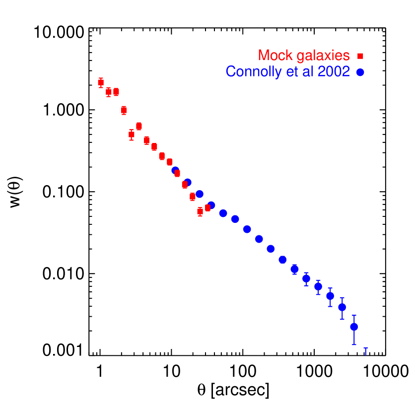
Figure 1.— Angular correlation function of mock galaxies (filled squares) compared to the angular correlation function of SDSS galaxies selected with $18<r^{\star}<22$, from Connolly et al. (2002) (filled circles).

In the case of both GALEX and SDSS, galaxies and stars show on average similar densities over the sky. We create a mock catalog over 100 sqdeg with a total of 10⁷ sources, half clustered and half random. The minimum Galactic latitude at which this mock catalog is representative is around 25^∘. For this case study we do not consider the variation of star density with Galactic latitude; we note that several mock catalogs can be constructed with different star densities, and prior probabilities (see sect. 3) varying accordingly.

2.2. Simulated Detections

From our mock catalog we create two sets of simulated detections, using the approximate astrometry errors of the surveys we consider. We assume that the errors are Gaussian, and create two detections for each mock object: a mock SDSS detection with $\sigma_{S}$, and a mock GALEX one with $\sigma_{G}$. We consider constant errors for SDSS, and variable errors for GALEX. For GALEX we focus here on the case of the Medium Imaging Survey (MIS); we will consider two selections: all MIS objects, or MIS objects with signal-to-noise ratio (S/N) larger than 3. We randomly assign to the mock sources errors from objects of the GALEX datasets following the relevant selections and using the position error in the NUV band (nuv_poserr). The distributions of these errors are shown on figure 2. In the case of GALEX, the position errors are defined as the combination of the Poisson error and the field error, added in quadrature. The latter is assumed to be constant over the field (and equal to 0.42″ in NUV). For SDSS we assume that $\sigma_{S}=0.1\arcsec$ for all objects. Our results are unchanged if we use variable SDSS errors for our SDSS mock detections, as the SDSS position errors are significantly smaller than the GALEX ones.

Figure 2.— Distribution of astrometry errors for simulated detections. The solid line shows errors on nuv detections for the selection of all GALEX MIS objects, and dotted line for the MIS objects with S/N $>3$. These distributions are normalized by their integrals.

2.3. Selection function and confusion

Our goal is to use the mock catalog described above as a predictive tool in order to assess the quality of the cross-identifications between two datasets, here GALEX and SDSS. Hence our mock catalog has to present similar properties than the data. In practice we need to include two effects: the selection functions of both catalogs in order to match the number density of the data, as well as the confusion of detections caused by the combination of the seeing and point spread functions.

To apply the selection function, we assign to each mock source a random number $u$, drawn from an uniform distribution, which represents the property of the objects. We use the values of $u$ to select the simulated detections we further consider to study a given case of cross-identification. The length of the interval in $u$ sets the density for a given mock catalog. Using the notations of Budavári & Szalay (2008), we computed the number of SDSS GR7 sources, $N_{\rm{SDSS}}$ and GALEX GR5, $N_{\rm{}GALEX}$, and scaled them to the area of our mock catalog. These numbers set the interval in $u$ for both detection sets. We then use the overlap between the intervals in $u$ to set the density of common objects, as set by the prior probability determined independently from the data (see sect. 3).

To simulate the confusion of the detections, we performed the cross-identification of the SDSS and GALEX detections sets with themselves, using a search radii of 1.5″ and 5″ respectively. These values of search radius correspond to the effective widths of the PSF in both surveys (Stoughton et al. 2002; Morrissey et al. 2007). We then consider only the detections that satisfy the selection function criterion, and merge them. For SDSS, we keep one source chosen randomly from the various identifications. For GALEX, we keep the source with the largest position error.

This procedure is repeated for each cross-identification we consider, as modifying the selection function naturally implies a change in the number densities and priors.

3. Cross identification

We performed the cross-identification between the SDSS and GALEX detection sets using a 5″ radius. For each association (see Budavári & Szalay 2008), we compute the Bayes factor

$$B(\psi;\sigma_{S},\sigma_{G})=\frac{2}{\sigma^{2}_{S}+\sigma^{2}_{G}}\exp\left[-\frac{\psi^{2}}{2(\sigma^{2}_{S}+\sigma^{2}_{G})}\right]$$ (1)

where $\psi$ is the angular separation between the two detections, and is expressed here in radians, as $\sigma_{S}$ and $\sigma_{G}$. We also derive the posterior probability that the two detections are from the same source

$$P=\left[1+\frac{1-P_{0}}{B\,P_{0}}\right]^{-1}\approx\frac{B\,P_{0}}{1+B\,P_{0}}$$ (2)

where $P_{0}$ is the prior probability, and the approximation is for the usually small priors.

The Bayes factor, and hence the posterior probability depend on the position errors from both surveys. As we use a constant prior $P_{0}$, this implies that if all objects have the same position errors within a survey, the posterior probability depends on the angular separation only. In this case, there is no difference between using a criterion based upon separation or probability.

We use the posterior probability rather than the Bayes factor as a criterion. In the assumption of a constant prior probability, the posterior probability is a monotonic function of the Bayes factor. However, while we consider here for our case study that the prior is a constant, in practice it may vary over the sky. Note also that for instance two surveys with similar position error distributions can have different priors and then a criterion defined on the basis of the Bayes factor for one survey can not be applied directly to the other one.

In order to set the overlap between our two detection sets as described in sect. 2.3 to match the selection functions of the actual datasets, we need to compute the prior $P_{0}$ from the data, using the actual cross-identification between GALEX GR5 and SDSS DR7.

The prior is given by

$$P_{0}=\frac{N_{\star}}{N_{SDSS}N_{GALEX}}.$$ (3)

$N_{\star}$ is the number of sources in the overlap between the various selections (angular, radial, etc …) of the catalogs considered for the cross identification, i.e. the number of sources in the resulting catalog. We use the self-consistency argument discussed by Budavári & Szalay (2008)

$$\sum P=N_{\star}$$ (4)

to derive $P_{0}$. To choose the value of the prior, we use the iterative process described in Budavári & Szalay (2008). We start the process by setting $N_{\star}=min(N_{SDSS},N_{GALEX})$. We then compute the sum of the posterior probabilities derived using eq. 2. According to eq. 4, this sum gives us a new value for $N_{\star}$. The same procedure is then repeated using this updated value, yielding an updated value of the prior as well. The chosen value for the prior is obtained after convergence; we hereafter call this value the observed prior.

Then we set the overlap between the two detection sets in our mock catalog such that the prior value derived for the cross-identification in the simulations matches the observed one. We use the same iterative process as described above to determine $P_{0}$ in the simulations. Figure 3 shows this iteration process starting from $N_{\star}=N_{\rm{}GALEX}$ for the case with all MIS objects (filled circles) or MIS S/N $>$3 objects (open circles). The procedure converges quickly in terms of number of steps. Note also that the query we use to compute the sum runs in roughly 1 second on these simulations.

The benefit of the use of simulations is that, in this case, once we set the overlap between the detection sets required to match the observed prior, we know the input value of $N_{\star}$ (i.e. the actual number of detections in the overlap between the two sets) and hence we can derive the prior corresponding to this number directly using eq. 3, which we call the true prior. We show this true prior on fig. 3 as solid line for the case of all MIS objects, and dashed line for MIS objects with S/N $>$3. The true priors we are required to use in order to match the data is slightly lower than the observed ones for both selections: 4% lower for all MIS objects and 2.5% for MIS objects with S/N $>$3. In other words, we need to use less objects in the overlap between our detection sets than what we expect from the data.

A different prior value implies a change in the posterior probability; however the latter also depends on the values of the Bayes factor $B$. Given the scaling of the relation between the posterior and prior probabilities (eq. 2), for low $B$ values ($B\ll 1$), a variation of 4% in the prior yields a variation in posterior probability of the same amount. For high $B$ values ($B\gg 1$), the variation is about 0.5%. Hence this difference between the true and observed priors has a negligible impact on the values of the posterior probabilities derived afterwards.

Figure 3.— Prior probability self-consistent estimation as a function of iteration step. Filled circles show the iteration for the case of all MIS objects, and open circles for MIS objects with S/N $>$3. The solid (dashed) line shows the true prior for all MIS objects (MIS objects with S/N $>$3).

To quantify the quality of the cross-identification, we define the true positive rate, $T$ and the false positive contamination, $F$. We can express these quantities as a function of the angular separation of the association, or the posterior probability. Let $n(x)$ be the number of associations, where $x$ denote separation or probability. This number is the sum of the true and false positive cross-identifications: $n(x)=n_{T}(x)+n_{F}(x)$. We define the true positive rate and false positive contamination as a function of angular separation as

$$T(\psi) = \frac{\sum n_{T}(x<\psi)}{N_{T}}$$ (5)

$$F(\psi) = \frac{\sum n_{F}(x<\psi)}{\sum n(x<\psi)}$$ (6)

where $N_{T}$ is the total number of true associations. Similar rates are defined as a function of the probability,

$$T(P) = \frac{\sum n_{T}(x>P)}{N_{T}}$$ (7)

$$F(P) = \frac{\sum n_{F}(x>P)}{\sum n(x>P)}.$$ (8)

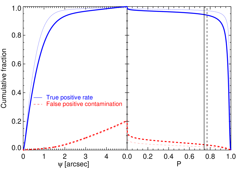
Figure 4.— True positive contamination rate (in blue, solid lines) and false positive contamination (red, dashed lines) as a function of angular separation (left) and posterior probability (right). GALEX position errors from the full MIS sample yield the thick curves; the S/N $>3$ constraint yields the thin curves. We also show the posterior probability thresholds defined as in Budavári & Szalay (2008) (vertical lines on right hand side plot).

We use the detection merging process to qualify the cross-identifications as true or false. In our final mock catalog, a detection represents a set of detections that have been merged. We therefore consider a case as a true cross-identification where there is at least one detection in common within the two sets of merged detections.

Figure 4 represents the true positive rate and the false contamination rate as a function of angular separation (left) and posterior probability (right). These results suggest that in the case of the SDSS GALEX-MIS cross-identification, it is required to use a search radius of 5″ in order to recover all the true associations. In the case of all MIS objects, 90% of the true matches are recovered at 1.64″ with a 2.6% contamination from false positive. As expected, results are better using objects with high signal-to-noise ratio (S/N $>$ 3), where 90% of the true matches are recovered at 1.15″ with a 1% contamination. Turning to the posterior probability, the trends are similar to the ones observed as a function of separation. However, the false positive contamination increases less rapidly with probability. For instance, a cut at $P>0.89$ recovers 90% of the true associations, with a slightly lower contamination from false positive (2.3%). We examine in details the benefits of using separation or probability as a criterion in Section 4.

4. Results

4.1. Performance analysis

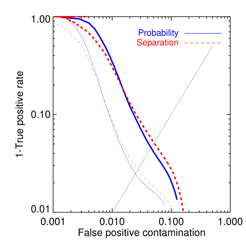
Figure 5.— Cross identification diagnostic plot: 1-true positive rate versus the false positive contamination. These quantities are computed as a function of probability (blue, solid lines) or separation (red, dashed lines). Thick lines show the results for all GALEX MIS objects, and thin lines for GALEX MIS objects with S/N $>3$. The dotted line represents the locus of $1-T=F$.

Using the quantities defined above, we can build a diagnostic plot in order to assess the overall quality of the cross-identification, and define a criterion to select the objects to use in practice for further analyses. We show on Fig. 5 the true positive rate against the false positive contamination, computed as a function of probability or angular separation. We can compare the false positive contamination that yields a given true positive rate threshold for each of these parameters.

The results show that there are some differences between criteria based on angular separation or posterior probability. Considering all GALEX MIS objects (solid lines on fig. 5), for $1-T>0.18$, the false contamination rate is slightly lower when using angular separation as a criterion. This range of true positive rates corresponds to angular separations smaller than 1.2″. As there is a lower limit to the GALEX position errors, this translates into an upper limit in terms of posterior probability at a given angular separation. This in turn implies that the probability criterion does not appear as efficient as separation for associations at small angular distances in the SDSS-GALEX case.

At $1-T<0.18$, this trend reverses: considering a criterion based on probability yields a lower false contamination rate.

We can characterize these diagnostic curves by the Bayes threshold, where $1-T=F$, which minimizes the Bayes error. The location of this threshold is represented on fig. 5 by the intersection between the diagnostic curves and the dotted line. Our results show that this intersection happens at lower false positive contamination rate when using the posterior probability as criterion.

For all GALEX objects, the separation where $1-T=F$, $\psi_{c}$, is equal to 2.307″ and the probability, $P_{c}$ is 0.613. Using the angular separation as criterion, the Bayes error is then $P_{e}=0.102$; using the posterior probability, $P_{e}=0.091$. For GALEX objects with S/N $>$3, $\psi_{c}=$1.882″, $P_{c}$ = 0.665; $P_{e}=0.055$ using the angular separation and $P_{e}=0.049$ using the posterior probability.

These results show that a selection based on posterior probability yields better results (i.e., a lower false contamination rate, and lower Bayes error) than a selection based on angular separation.

4.2. Associations

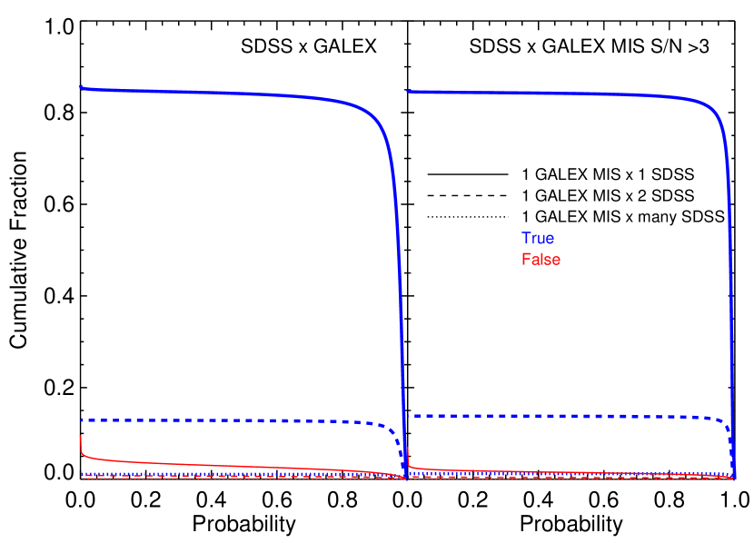
Figure 6.— True positive rate (blue, thick lines) and false contamination rate (red, thin lines) as a function of probability for the one GALEX to one SDSS (solid lines), one GALEX to two SDSS (dashed lines), one GALEX to many SDSS (dotted lines) associations. The left panel show these rates for all GALEX MIS objects, and the right one for the GALEX MIS objects with S/N $>$3. Note that the curves representing the one GALEX to many SDSS associations can barely be seen as the value are too small.

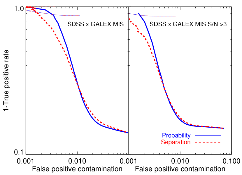
Figure 7.— 1-True positive rates as a function of the false contamination rate for the one GALEX to one SDSS (thick lines) and one GALEX to two SDSS (thin lines) associations. The rates are computed as a function of probability (blue, solid lines) or separation (red, dashed lines). The left panel show these rates for all GALEX MIS objects, and the right one for the GALEX MIS objects with S/N $>$3.

Table 1Percentages of associations by type

SDSS
GALEX	1	2	Many
1	74.061 (75.870)	21.007 (18.595)	2.577 (2.469)
2	1.146 (2.253)	1.006 (0.697)	0.188 (0.102)
Many	0.006 (0.009)	0.007 (0.004)	0.002 (0.001)

Note. — Percentages of associations by type in the mock catalogs. The numbers in brackets give the percentages from the cross-identification of SDSS DR7 and GALEX GR5 data. All percentages are given with respect to the total number of matches.

Beyond the confused objects, the cross-identification list contains several types of associations, where a single detection in one catalog is linked to possibly more than one detection in the other. We list in table 1 the contingency table of the percentages of these types in the mock catalog and, in brackets, for the SDSS DR7 to GALEX GR5 cross-identifications.

The main contribution is from the one GALEX to one SDSS (1G1S, 74%), but there are also, for the most significant ones, cases of one GALEX to two SDSS (1G2S, 21%) or one GALEX to many SDSS (1GmS, 3%). Comparing with the data, our mock catalogs are slightly pessimistic in the sense that the fraction of one to one matches is lower than in the observations. However, these fractions match reasonably well enough, which enables us to discuss these cases in the context of our mock catalogs. We show on figure 6 the true positive and false contamination rates as a function of probability for the 1G1S (solid lines), 1G2S (dashed lines), and 1GmS (dotted lines) associations. The 1G1S true associations represent the bulk (up to 85%) of the total cross-identifications. There is also a significant fraction of true associations within the one 1G2S cases (up to nearly 13%), while the 1GmS are around 1%. For the 1G2S or 1GmS cases, we use two methods to select one object among the various associations: the one corresponding to the highest probability or the smallest separation. We computed the true positive and false contamination rates for these cases as a function of the quantity used for the selection of the association. We compare the results from these two methods on figure 7, which shows the diagnostic curves for the 1G1S (thick lines), 1G2S (thin lines); we do not show here the 1G2m as they represent only 1% of the associations. The diagnostic curves present the same trend than the global ones (see Fig. 5): the posterior probability criterion yields a lower false contamination rate than the angular separation criterion above some true positive rate value (e.g., $1-T<0.29$, for 1G1S associations considering the cross-identification of all SDSS GALEX objects).

This is however an artifact caused by the distribution of the GALEX position errors (see sect. 4.1). For the 1G2S or 1GmS cases, these results show that true associations can be recovered by selecting maximal probability, with a low contamination from false positive (up to around 1%).

On Figs. 6 and 7 we compare the results from all GALEX MIS objects and GALEX MIS objects with S/N $>$ 3. The quality of the cross-identifications are better for the latter, for all types of associations.

4.3. Alternative Error model

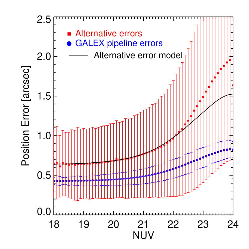
Figure 8.— GALEX position error as a function of NUV magnitude. Circles show the GALEX pipeline error, squares the alternative errors (see text). The solid line show the linear model we use to modify the GALEX pipeline errors.

The accuracy of the analysis of the quality of the cross-identification strongly depends on the GALEX pipeline position errors. We use the real data, namely the angular separation to the SDSS sources measured during the cross-identification between GALEX GR5 and SDSS DR7, to get an alternative estimation of realistic errors. In principle the distribution of the angular separations of the associations depends on the combination of the GALEX and SDSS position errors. However, the latter are significantly smaller than the former, so we consider the SDSS errors as negligible here. We compare on figure 8 the dependence on the NUV magnitude of the position error in the NUV band from the GALEX pipeline (circles on fig. 8) and the distance to the SDSS sources (squares), considering only objects classified as point sources in SDSS. The angular separation between the sources of the two surveys are significantly larger than the quoted GALEX pipeline errors. These latter errors are a combination of a constant field error (equal in NUV to 0.42″) and a Poisson term. In the range where both errors estimates are constant ($18<$NUV$<20$), this comparison suggests that the GALEX field error might be slightly underestimated. Fot fainter objects, our alternative error increase faster with magnitude than the GALEX pipeline errors, which might indicate that this dependence is not well reproduced by the Poisson term.

We fitted a linear relation to modify the GALEX errors in order to match the angular separations to the SDSS sources

$$\textrm{NUV}^{mod}_{poserr}=2.2\textrm{NUV}_{poserr}-0.3$$ (9)

where the position errors are in units of arcsec. This error model is shown as a solid line on figure 8. It reproduces well the alternative errors for NUV $\lesssim 22.5$, which is similar to the 5$\sigma$ limiting magnitude for the MIS in the NUV band (22.7; Morrissey et al. 2007).

We followed the same steps as described in sect. 2.2 and 2.3 with these new errors and performed the cross-identification. The diagnostic curves we obtain are presented on Fig. 9.

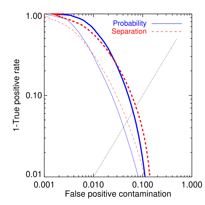
Figure 9.— Same as figure 5 using alternative position errors for GALEX sources (see text).

The trends are similar to those observed using the GALEX pipeline errors. The quality of the cross-identification is nevertheless worse with the alternate errors. In this case, the values of angular separation and probability where $1-T=F$ are $\psi_{c}=3.126\arcsec$, $P_{c}=0.711$ for all GALEX objects. Using the angular separation as a criterion, $P_{e}=0.144$ (0.102 with the GALEX pipeline error), and $P_{e}=0.127$ (0.091 with pipeline errors) with the posterior probability. For GALEX objects with S/N $>$ 3, $\psi_{c}=2.514\arcsec$, $P_{c}=0.780$ ; $P_{e}=0.0958$ (0.055, pipeline errors) using angular separation, and $P_{e}=0.0812$ (0.049, pipeline errors) with the posterior probability.

In other words, the contamination from false positive is larger at a given true positive rate. For instance, for all GALEX MIS objects, with 90% of the true associations and considering posterior probability as a criterion, the contamination is 5% compared to 2.3% using the GALEX pipeline errors. Note also that the difference between the angular separation and the probability diagnostic curves is larger with this alternate error model. This suggests that the probability is a more efficient way than angular separation to select cross-identifications for surveys with larger position errors.

4.4. Building a GALEX-SDSS catalog

Table 2Selection criteria for SDSS-GALEX sample

Association	Probability cut	False positive contamination
1 GALEX to 1 SDSS	$P>0.877$	1.6
1 GALEX to 2 SDSS	$P>0.955$	0.2
1 GALEX (S/N $>$ 3) to 1 SDSS	$P>0.939$	0.7
1 GALEX (S/N $>$ 3) to 2 SDSS	$P>0.982$	0.1

Note. — Posterior probability cuts to obtain 80% (10%) of the true associations for the one GALEX to one SDSS (one GALEX to two SDSS) matches. The corresponding false positive contamination percentages are also listed. The first two lines give the cuts for all GALEX MIS objects and the two last ones for the GALEX MIS objects with S/N $>$ 3.

The combination of the results we presented can be used to define a set of criteria for constructing a reliable joint GALEX-SDSS catalog. It is natural to have different selections for each type of association. We will here focus on the 1G1S and 1G2S cases, as they represent around 95% of the associations.

In Table 2 we propose a set of criteria, based on the posterior probability, to get 90% of the true cross-identifications, consisting of 80% of 1G1S and 10% of 1G2S. We also list the corresponding false positive contamination. These cuts enable to build catalogs with 1.8% of false positives when using all GALEX objects, or 0.8% when using GALEX objects with S/N $>3$.

5. Conclusions

We presented a general method using simple mock catalogs to assess the quality of the cross-identification between two surveys which takes into account the angular distribution and confusion of sources, and the respective selection functions of the surveys. We applied this method to the cross-identification of the SDSS and GALEX sources. We used the probabilistic formalism of Budavári & Szalay (2008) to study how the quality of the associations can be quantified by the posterior probability. Our results show that criteria based on posterior probability yield lower contamination rates from false positive than criteria based on angular separation. In particular, the posterior probability is more efficient than angular separation for surveys with larger position errors. Our study also suggest that the GALEX pipeline position errors might be underestimated and we described an alternative measure of these errors. We finally proposed a set of selection criteria based on posterior probability to build reliable SDSS-GALEX catalogs that yield 90% of the true associations with less than 2% contamination from false positives.

6. Acknowledgements

The authors gratefully acknowledge support from the following organisations: Gordon and Betty Moore Foundation (GMBF 554), W. M. Keck Foundation (Keck D322197), NSF NVO (AST 01-22449), NASA AISRP (NNG 05-GB01G), and NASA GALEX (44G1071483).

References

- Budavári & Szalay (2008) Budavári, T., & Szalay, A. S. 2008, ApJ, 679, 301
- Connolly et al. (2002) Connolly, A. J., et al. 2002, ApJ, 579, 42
- Davis et al. (2007) Davis, M., et al. 2007, ApJ, 660, L1
- Dickinson et al. (2003) Dickinson, M., Giavalisco, M., & The Goods Team 2003, The Mass of Galaxies at Low and High Redshift, 324
- Martin et al. (2005) Martin, D. C., et al. 2005, ApJ, 619, L1
- Morrissey et al. (2007) Morrissey, P., et al. 2007, ApJS, 173, 682
- Pons-Bordería et al. (1999) Pons-Bordería, M.-J., Martínez, V. J., Stoyan, D., Stoyan, H., & Saar, E. 1999, ApJ, 523, 480
- Scoville et al. (2007) Scoville, N., et al. 2007, ApJS, 172, 1
- Stoughton et al. (2002) Stoughton, C., et al. 2002, AJ, 123, 485
- York et al. (2000) York, D. G., et al. 2000, AJ, 120, 1579