Multicriticality in the Blume-Capel model under a continuous-field probability distribution

Abstract

The multicritical behavior of the Blume-Capel model with infinite-range interactions is investigated by introducing quenched disorder in the crystal field $\Delta_{i}$, which is represented by a superposition of two Gaussian distributions with the same width $\sigma$, centered at $\Delta_{i}=\Delta$ and $\Delta_{i}=0$, with probabilities $p$ and $(1-p)$, respectively. A rich variety of phase diagrams is presented, and their distinct topologies are shown for different values of $\sigma$ and $p$. The tricritical behavior is analyzed through the existence of fourth-order critical points, as well as how the complexity of the phase diagrams is reduced by the strength of the disorder.

Keywords: Random-Field Blume-Capel Model; Mean-Field Approach; Tricritical Behavior.

I Introduction

The effect of disorder on different types of condensed matter orderings is nowadays a subject of considerable interest binder ; ghosal . For the case of disordered magnetic systems, random-field spin models have been systematically studied, not only for theoretical interests, but for some identifications with experimental realizations belanger . An interesting issue, is the study of how quenched randomness destroys some types of criticalities. So, in what concerns the effect produced by random fields in low dimensions, it has been noticed hui ; berker that first-order transitions will be replaced by continuous transitions, so tricritical points and critical end points will be depressed in temperature, and a finite amount of disorder will suppresse them. Nevertheless, in two dimensions, an infinitesimal amount of field randomness seems to destroy any first-order transition wehr ; boechat . Interestingly, the simplest model exhibiting a tricritical phase diagram in the absence of randomness is the Blume-Capel model. The Blume-Capel model blume ; capel is a regular Ising model for spin-1 used to model $\bf{}^{4}He-^{3}He$ mixturesemeryg . The interesting feature is the existence of a tricritical point in the phase diagram represented in the plane temperature versus crystal field, as shown in Figure 1. This phase diagram was firslty obtained in the mean-field approach, but the same qualitative properties were also observed in low dimensions. The latter was confirmed through some approximation techniques as well as by Monte Carlo simulations mahan ; jain ; grollau ; kutlu ; seferoglu . Also, the tricritical behavior is still held in two dimensions clusel ; care ; paul ; caparica . Nevertheless, in other models this situation is controversial. For example, the random-field Ising Model in the mean-field approach aharony also exhibits a tricritical point, but some Monte Carlo simulations fytas in the cubic lattice suggest that this is only an artifact of the mean-field calculations. Accordingly, this interesting fact in the Blume-Capel model motivated some authors to explore the richness of this model, within the mean-field approach, by introducing disorder in the crystal field hamid ; benyoussef ; salinas ; carneiro as well as by adding and external random field miron . For the former case, it was obtained a variety of phase diagrams including different critical points with some similar topologies found for the random-field spin$-1/2$ Ising model kaufman ; octavio . However, in those studies the fourth-order critical points, which limit the existence of tricritical points, were overlooked. Consequently, our aim in this work is to improve those previous studies by considering a more general probability distribution function for the crystal field, and bettering some results given in references benyoussef ; salinas ; carneiro . The next section is dedicated to define the model and the special critical points produced by it.

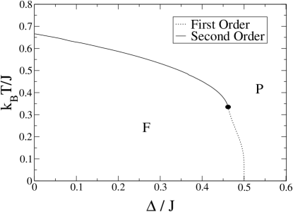
Figure 1: Phase diagram of the Blume-Capel model in the plane $k_{B}T/J-\Delta/J$ within the mean-field approach, where $k_{B}$ is the Boltzman constant, $T$ is the temperature, $J>0$ is the coupling constant between each pair of spins, and $\Delta$ is the crystal field (also called the anisotropy field). The black circle represents the tricritical point. The Ferromagnetic and Paramagnetic phases are represented by $\bf F$ and $\bf P$, respectively. The full line represents the continuous or second-order critical frontier, and the dotted line is for the first-order frontier.

II The Model

The infinite-range-interaction Blume-Capel model is given by the following Hamiltonian

$${\cal H}=-\frac{J}{N}\sum_{(i,j)}S_{i}S_{j}+\sum_{i}\Delta_{i}S_{i}^{2}~{},$$ (1)

where $S_{i}=-1,0,1$, and $N$ is the number of spins. The first sum runs over all distinct pairs of spins. The coupling constant $J$ is divided by $N$ in order to maintain the extensivity. The crystal fields are represented by quenched variables $\{\Delta_{i}\}$, obeying the probability distribution function (PDF) given by,

$$P(\Delta_{i})=\frac{p}{\sqrt{2\pi}\,\sigma}\exp\left[-\frac{(\Delta_{i}-\Delta)^{2}}{2{\sigma}^{2}}\right]+\frac{(1-p)}{\sqrt{2\pi}\,\sigma}\exp\left[-\frac{{\Delta_{i}}^{2}}{2{\sigma}^{2}}\right]~{},$$ (2)

which consists of a superposition of two independent Gaussian distributions with the same width $\sigma$, centered at $\Delta_{i}=\Delta$ and $\Delta_{i}=0$, with probabilities $p$ and $(1-p)$, respectively. For $\sigma=0$, we recover the bimodal distribution studied in references benyoussef ; salinas , and for $p=1$, the simple Gaussian one of reference carneiro . For $\sigma=0$ and $p=1$, we go back to the simple Blume-Capel model without randomnessemeryg .
By standard procedures octavio , we get the analytical expression for the free energy per spin ($f$), through which may be obtained a self-consistent equation for the magnetization $m$. Thus, we have the following relations at the equilibrium,

$$f=\frac{1}{2}Jm^{2}-\frac{1}{\beta}E\left\{\log(2\exp(-\beta\Delta_{i})\cosh(\beta Jm)+1)\right\}~{},$$ (3)

$$m=\sinh(\beta m)E\left\{{\left[\cosh(\beta m)+\frac{1}{2}\exp(\beta\Delta_{i})\right]}^{-1}\right\}~{},$$ (4)

where the quenched average, represented by $E\{...\}$, is taken with respect to the PDF given in Eq. (2), and $\beta=1/(k_{B}T)$. To write conditions for locating tricritical and fourth-order critical points, we expand the right hand of Eq. (4) in powers of $m$ (Landau’s expansion, see stanley ). Conveniently, we expand the magnetization up to seventh order in $m$, so

$$m=A_{1}m+A_{3}m^{3}+A_{5}m^{5}+A_{7}m^{7}+...~{},$$ (5)

where

$$A_{1}=\beta E\{g_{i}\}~{},$$ (6)

$$A_{3}=\beta^{3}E\{(\frac{1}{6}g_{i}-\frac{1}{2}g_{i}^{2})\}~{},$$ (7)

$$A_{5}=\beta^{5}E\{(\frac{1}{120}g_{i}-\frac{1}{8}g_{i}^{2}+\frac{1}{4}g_{i}^{3})\}~{},$$ (8)

$$A_{7}=\beta^{7}E\{(\frac{1}{5040}g_{i}-\frac{1}{80}g_{i}^{2}+\frac{1}{12}g_{i}^{3}-\frac{1}{8}g_{i}^{4})\}~{},$$ (9)

and

$$g_{i}=(1+\frac{1}{2}\exp(\beta\Delta_{i}))^{-1}~{}.$$ (10)

In order to obtain the continuous critical frontier one sets $A_{1}=1$, provided that $A_{3}<0$. If a first-order critical frontier begins after the continuous one, the latter line ends at a tricritical point if $A_{3}=0$, provided that $A_{5}<0$. The possibility of a fourth-order critical point is given for $A_{1}=1$, $A_{3}=0$, $A_{5}=0$ and $A_{7}<0$. Thus, a fourth-order point may be regarded as the last tricritical point.
By taking $\beta\to\infty$ ($T\to 0$), we get the asymptotic limit of Eqs. (3) and (4), so we have

$$f = \frac{1}{2}Jm^{2}-p\left(\frac{1}{2}(Jm-\Delta)\left(1+{\rm erf}\left[\frac{Jm-\Delta}{\sqrt{2}\,\sigma}\right]\right)+\frac{\sigma}{\sqrt{2\pi}}\exp\left[-\frac{(Jm-\Delta)^{2}}{2\,{\sigma}^{2}}\right]\right)$$ (11)

$$- (1-p)\left(\frac{1}{2}Jm\left(1+{\rm erf}\left[\frac{Jm}{\sqrt{2}\,\sigma}\right]\right)+\frac{\sigma}{\sqrt{2\pi}}\exp\left[-\frac{J^{2}m^{2}}{2\,{\sigma}^{2}}\right]\right)~{},$$

$$m=\frac{p}{2}\left(1+{\rm erf}\left[\frac{Jm-\Delta}{\sqrt{2}\,\sigma}\right]\right)+\frac{(1-p)}{2}\left(1+{\rm erf}\left[\frac{Jm}{\sqrt{2}\,\sigma}\right]\right)~{},$$ (12)

where

$${\rm erf}\left(\frac{x}{\sqrt{2}}\right)=\sqrt{\frac{2}{\pi}}\int_{0}^{x}dze^{-z^{2}/2}~{}.$$ (13)

The critical frontiers, for a given pair $(\sigma,p)$, are obtained by solving a non-linear set of equations, which consist of equating the free energies for the corresponding phases (Maxwell’s construction), and the respective magnetization equations based on the relations given in Eqs. (3), and (4). We must carefully verify that every numerical solution minimizes the free energy.
The symbols used to represent the different critical lines and points octavio are as follows:

• Continuous or second-order critical frontier: continuous line;

• Fist-order critical frontier: dotted line;

• Tricritical point: located by a black circle;

• Fourth-order critical point: located by an empty square;

• Ordered critical point: located by an asterisk;

• Critical end point: located by a black triangle.

To clarify, we mean by a continuous critical frontier that which separates two distinct phases through which the order parameter changes continuously to pass from one phase to another, contrary to the case of the first-order transition, through which, the order parameter suffers a discontinuous change, so the two corresponding phases coexist at each critical point. A tricritical point is basically the point in which a continuous line terminates to give rise a first-order critical line. A fourth-order critical point is sometimes called a vestigial tricritical point, because it may be regarded as the last tricritical point. An ordered critical point is the point, inside an ordered region, where a first-order critical line ends, above which the order parameter passes smoothly from one ordered phase to the other. Finally, a critical end point corresponds to the intersection of a continuous line that separates the paramagnetic from one of the ferromagnetic phases with a first- order line separating the paramagnetic and the other ferromagnetic phase. In following section we make use of this definitions.

III Results and Discussion

The distinct phase diagrams for the present model were numerically obtained by scanning the whole p-domain for each $\sigma$-width. So, distinct topologies belonging to different $p$-ranges were found for a given $\sigma$. For instance, Figure 2 shows the whole variety of them for a small $\sigma/J=0.1$, for each arbitrary representative $p$.

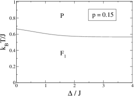
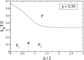
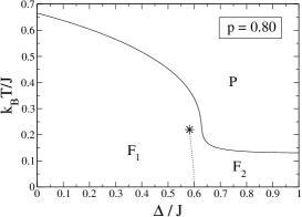
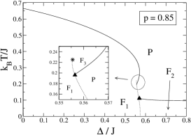
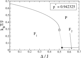
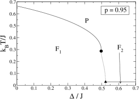
Figure 2: Phase diagrams of the Blume-Capel Model whose crystal field obeys the PDF given in Eq.(2). For $\sigma/J=0.1$, the diagrams show a variety of topologies according to the probability $p$. For convenience, we classify them in four topologies, so in (a) is shown Topology I; in (b) and (c) Topology II; in (d) Topology III, then figures (e) and (f) represent Topology IV.

Note that for small values of $p$, one only ferromagnetic order appears at low temperatures, as shown in Figure 2(a) for $p=0.15$. We designate it as Topology I. Figures 2(b) and (c) ($p=0.5,0.8$) represent the same topology (Topology II), which consists of one first-order critical line separating two different ferromagnetic phases $\bf F_{1}$ and $\bf F_{2}$, and a continuous line remaining for $\Delta/J\to\infty$. Figure 2(c), though qualitatively the same as in 2(b), is intended to show how the first-order line and the continuous line approach themselves as $p$ increases. Figure 2(d) shows Topology III, for $p=0.85$, so the preceding first-order line is now dividing the continuous line by two critical end points. Note that the upper continuous line terminates, following a reentrant path, at a critical end point where the phases $\bf F_{1}$, $\bf F_{3}$, and $\bf P$ coexist. So, at the lower critical end point, $\bf F_{1}$, $\bf F_{2}$, and $\bf P$ coexist. Above the ordered critical point, the order parameter passes smoothly from $\bf F_{1}$ to $\bf F_{3}$ (see the inset there). If we increase $p$ up to some $p=p^{*}$, the upper continuous line and the first-order line will be met by a fourth-order point (represented by a square) as shown in Figure 2(e). Thus, $p^{*}$ is the threshold for Topology IV. Then, for $p>p^{*}$, those lines will be met at a tricritical point, as noticed in Figure 2(f). Conversely, tricritical points appear for $p>p^{*}$, so the last one for $p=p^{*}$. The same types of phase diagrams are found in references benyoussef ; salinas ; carneiro . Nevertheless, we improve their results, not only bettering some of their numerical calculations, but in that we may now locate the regions of validity of these topologies in the plane $\sigma/J-p$. To this end, we start by locating the fourth-order points in the plane $\sigma/J-p$, as shown in Figure 3.

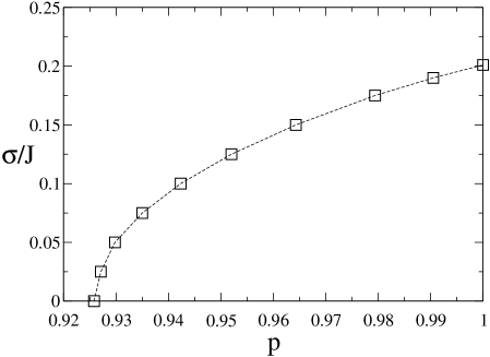
Figure 3: Some fourth-order critical points located in the plane $p-\sigma/J$. Note that if $\sigma=0$, we recover the bimodal case studied in references benyoussef ; salinas , where we found $p^{*}=0.9258$, just in agreement with them. Note that if $p=1$, $\sigma/J=0.202$, so it is a $\sigma$-limit for the tricritical behavior. The dashed line is only a guide to the eyes.

Note that $\sigma/J=0.202$ is a cut-off for the tricritical behavior. Then, Topology IV will no longer found for greater widths. On the other hand, we determine the threshold for Topology III, by estimating numerically which value of $p$, for each $\sigma/J$, produces a situation like that presented in Figure 4 (case $\sigma/J=0.1$), where we see how Topology III emerges for a $p$ slightly greater than $0.836$. For $\sigma/J=0$, we found this threshold for $p=0.8245$, which is smaller than that obtained in reference benyoussef . There, the authors suggested that Topology III disappears for $p<8/9=0.888...$ . However, Figure 5 illustrates that this type of phase diagram is still present even for a smaller $p$, as confirmed by the free energy evaluated at three disctinct ($k_{B}T/J,\Delta/J$)-points along the first-order critical line, at which there are three types of coexistences, namely, $\bf F_{1}$ with $\bf F_{3}$, $\bf F_{1}$ with $\bf P$, and $\bf F_{1}$ with $\bf F_{2}$. We also noted another discrepancy with respect to a critical $\sigma/J$, found in reference carneiro , above which Topology III disappears for $p=1$. There, the authors affirmed that if $\sigma/J>0.229$, the paramagnetic-ferromagnetic transition becomes second order at all temperatures, but we noticed that it only happens for a greater width, namely, $\sigma/J=0.283$.
In order to obtain the frontier which separates Topologies I and II (in the plane $\sigma/J-p$), we have to find the corresponding $p$, for a given $\sigma/J$, that locates the one ordered critical point at $T=0$. To this end, the next subsection is focused on zero temperature calculations.

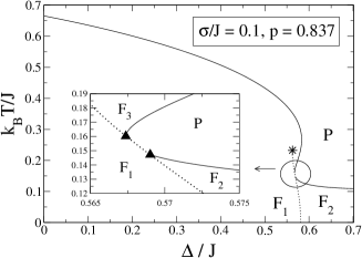
Figure 4: Phase diagrams (for $\sigma/J=0.1$) showing two slightly different values of $p$, between which there is a critical $p$ for passing from Topology II to III. So, that critical point must be found for $p=0.8365\pm 0.0005$.

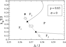
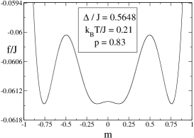
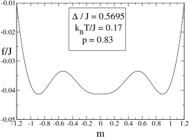
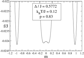
Figure 5: In (a) is shown the most critical region of the phase diagram for $\sigma=0$, and $p=0.83$. It is a typical phase diagram for Topology III (like that of Figure 2(d)). Note that three points belonging to the first-order critical line are highlighted by an ellipse, a rectangle, and a circle. The ellipse is surrounding a critical point where the phases $\bf F_{1}$ and $\bf F_{3}$ coexist, as confirmed through the free energy versus the magnetization in (b). In (c) and (d) the free energy shows which phases are coexisting at the points surrounded by the rectangle and the circle. Thus, in (c), the phases $\bf F_{1}$ and $\bf P$ coexist, because two symmetric minima at finites values of $m$, and one minimum at $m=0$, are at the same level. In (d), like in (b), are shown four symmetric minima at the same level. Therefore, the phases $\bf F_{1}$ and $\bf F_{2}$ coexist at this critical point.

III.1 Analysis at $T=0$

In order to perform zero temperature calculations we make use of the equations (11) and (12). Consequently, for $\sigma/J=0$ (see reference salinas ), there are two ferromagnetic phases $\bf F_{1}$ and $\bf F_{2}$ coexisting at $\Delta/J=1-p/2$, having magnetizations $m_{1}=1$ and $m_{2}=1-p$, respectively. We observed that these relations still remain up to some finite $\sigma$, after which a $\sigma$-dependency emerges. So, for a greater width called $\sigma^{{}^{\prime}}$, the ordered critical point (that of Topology III) must be found at $T=0$. Then, the first-order critical line is supressed and one only ferromagnetic order exists for any $p$. For instance, if we choose $p=0.5$, we find $\sigma^{{}^{\prime}}/J=0.2$, as illustrated in Figure 6. There, the zero temperature free energy versus the order parameter is plotted for three different values of $\sigma/J$, at the point where $\bf F_{1}$ and $\bf F_{2}$ coexist. Thus, In (a), two minima are at the same level for $\sigma=0.1$. In (b), it still happens for $\sigma=0.15$. Nonetheless, in (c), for $\sigma/J=0.2$, the ordered critical point is already at $T=0$. Therefore, for this particular $p$, there is only one ferromagnetic phase for $\sigma/J>0.2$.

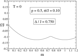
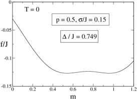
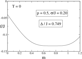
Figure 6: The Free energy (see Eq. (11)) versus the order parameter, plotted for $p=0.5$, for three different values of $\sigma/J$. In (a) and (b) two ferromagnetic phases coexist, but in (c) we note that for $\sigma/J=0.2$, there is already a crossover to pass from one ferromagnetic phase to the other.

For completeness, Figure 7(a) shows what Figure 6(c) illustrates by means of the free energy. There, it is shown where the ordered critical point is located, that is, at $T=0$. In Figure 7(b), we see the line composed by the $(p,\sigma^{{}^{\prime}}/J)$-points. This line separates phase diagrams containing two and one ferromagnetic phases. Particularly, for $p=1$, $\sigma^{{}^{\prime}}/J=(2\pi)^{-1/2}$, as obtained in reference carneiro and confirmed numerically by us.
We summarize the preceding analysis by showing, in Figure 8, the regions of validity for the four qualitatively distinct phase diagrams. Note that along the horizontal axis ($\sigma/J=0$), regions II and III are separated by $p=0.8245$, and regions III and IV by $p=0.9258$. Along the vertical axis (at $p=1$), regions IV and III are separated by $\sigma/J=0.202$, regions III and II by $\sigma/J=0.283$, then, regions II and I by $\sigma/J=(2\pi)^{-1/2}\approx 0.3989$. Furthermore, the line separating topologies I and II is the same as in Figure 7(b). The frontier separating topologies II and III consists of points estimated by the analysis illustrated by Figure 4. Finally, the line between topologies III and IV is made of fourth-order critical points, i.e., it is based upon the points in Figure 3.

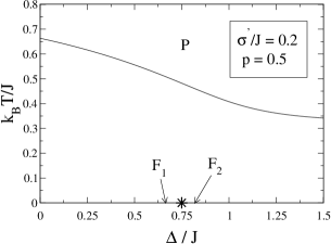
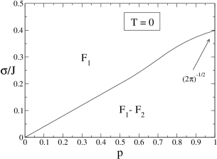
Figure 7: In (a) is shown the phase diagram obtained for $p=0.5$, for the corresponding critical $\sigma^{{}^{\prime}}/J$. Note that the ordered-critical point (that appeared in Topology II) is now located at the horizontal axis. So, for $\sigma>\sigma^{{}^{\prime}}$ there will be only one ferromagnetic order at low temperatures for $p=0.5$. In (b), the line separating topologies I and II. This line is made of points numerically obtained by finding $\sigma^{{}^{\prime}}/J$, for each $p$.

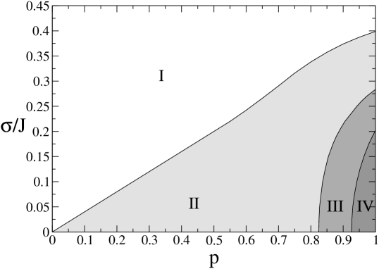
Figure 8: Regions, in the plane $\sigma/J$ versus $p$, associated with the topologies for the present model (see also Figure 2). The horizontal and the vertical axes represent the probability $p$, and the width $\sigma$, respectively (see Eq. (2)). The tricritical behavior belongs to the region IV. The simplest topology belongs to region I, where only one ferromagnetic phase appears, whereas the rest topologies contain two ferromagnetic orders at low temperatures.

IV Conclusions

We revisiting the study of the infinite-range-interaction spin-1 Blume-Capel Model with quenched randomness, by considering a more general probability distribution function for the crystal field $\Delta_{i}$, which consists of two Gaussian distributions centered at $\Delta_{i}=\Delta$ and $\Delta_{i}=0$, with probabilities $p$ and $(1-p)$, respectively. For $\sigma=0$, we recover the bimodal case studied in references benyoussef ; salinas , and for $p=1$, the Gaussian case studied in reference carneiro . For $\sigma$-widths in $0<\sigma<0.202J$, the system exhibits four distinct topologies according to the range in which $p$ belongs. So, we designed them as Topology I,II,III, and IV, in increasing order of $p$. Topology I contains one continuous critical line separating a ferromagnetic phase to the paramagnetic phase. In Topology II, one first-order critical line separating two ferromagnetic phases is added. This line terminates at an ordered critical point. The most complex criticality belongs to Topology III, where the first-order line now divides the continuous critical line by two critical end points. In Topology IV, the first-order line and the continuous line are met by a tricritical point. Accordingly, Topology I presents one ferromagnetic phase, whereas the rest ones show two distinct ferromagnetic orders at low temperatures. On the other hand, the tricritical behavior manifested in Topology IV emerges for $p>p^{*}$, where $p^{*}$ denotes the probability for a given $\sigma/J$, where a fourth-order critical point is found. This point may be regarded as the last tricritical point vanishing for $\sigma/J>0.202$, since $\sigma/J=0.202$ leads to $p^{*}=1$. Consequently, the tricritical behavior is no longer found for any $p$. Topology III disappears for $\sigma/J>0.283$, and Topology II is limited by $\sigma/J=0.3989$, above which the first-order line separating the two ferromagnetic phases is suppressed for any $p$. After that, for $\sigma/J>0.3989$, only the simplest topology survives.

Therefore, we show through this model how a complex magnetic criticality is reduced by the strength of the disorder (see also octavio ; crokidakisa ; crokidakisb ). Nevertheless, the critical dimensions for these types of phase diagrams is still an open problem to be solved.

Acknowledgments

Financial support from CNPq (Brazilian agency) is acknowledged.

References

- (1) K. Binder and A. P. Young, Rev. Mod. Phys. 58, 801 (1986).
- (2) A. Ghosal, M. Randeria, and N. Trivedi, Phys. Rev. Lett. 81, 3940 (1998).
- (3) D. P. Belanger, Spin Glasses and Random Fields, edited by A.P. Young (World Scientific, Singapore, 1998).
- (4) K. Hui and A. N. Berker, Phys. Rev. Lett. 62, 2507 (1989).
- (5) A. N. Berker, J. Appl. Phys. 70, 5941 (1991).
- (6) M. Aizenman and J. Wehr, Phys. Rev. Lett. 62, 2503 (1989).
- (7) N. S. Branco and B. M. Boechat, Phys. Rev. B 56, 11673 (1997).
- (8) M. Blume, Phys.Rev. 141, 517 (1966).
- (9) H. W. Capel, Physica (Utr.) 32, 966 (1966).
- (10) M. Blume, V. J. Emery, and R. B. Griffiths, Phys. Rev. A 4, 1071 (1971).
- (11) G. D. Mahan and S. M. Girvin, Phys. Rev. B 17, 4411 (1978).
- (12) A. K. Jain and D. P. Landau, Phys. Rev. B 22, 445 (1980).
- (13) S. Grollau, E. Kierlik, M. L. Rosinberg, and G. Tarjus, Phys. Rev. E 63, 041111 (2001).
- (14) B. Kutlu; A. Ozkan ; N. Seferogu; A. Solak, B. Binal, Int. J. Mod. Phys. B, 16, 933 (2005).
- (15) N. Seferoglu, A. Ozkan and B. Kutlu, Chinese Phys. Lett. 23, 2526 (2006).
- (16) M. Clusel, J.-Y. Fortin and V. N. Plechko, J. Phys. A: Math. Theor. 41, 405004 (2008).
- (17) C. M. Care, J. Phys. A 26, 1481 (1993).
- (18) P. D. Beale, Phys. Rev. B 33, 1717 (1985).
- (19) C. J. Silva and A. A. Caparica, Phys. Rev. E 73, 036702 (2006).
- (20) A. Aharony, Phys. Rev. B 18, 3318 (1978).
- (21) N. G. Fytas, A. Malakis, and K. Eftaxias, J. Stat. Mech. P03015 (2008).
- (22) H. Ez-Zahraouy and A. Kassou-Ou-Ali, Phys. Rev. B 69, 064415 (2004).
- (23) A. Benyoussef, T. Biaz, M. Saber and M. Touzani, J. Phys. C 20, 5349 (1987).
- (24) C. E. I. Carneiro, V. B. Henriques and S. R. Salinas, J. Phys.: Condens. Matter 1, 3687 (1989).
- (25) C. E. I. Carneiro, V. B. Henriques and S. R. Salinas, J. Phys. A: Math. Gen. 23, 3383 (1990).
- (26) M. Kaufman and M. Kanner, Phys. Rev. B 42, 2378 (1990).
- (27) M. Kaufman, P. E. Kluzinger and A. Khurana, Phys. Rev. B 34, 4766 (1986).
- (28) O. R. Salmon, N. Crokidakis and F. D. Nobre, J. Phys.: Condens. Matter 21, 056005 (2009).
- (29) H. E. Stanley, Introduction to Phase Transitions and Critical Phenomena (Clarendon Press, Oxford, 1971).
- (30) N. Crokidakis and F. D. Nobre, Phys. Rev. E 77, 041124 (2008).
- (31) N. Crokidakis and F. D. Nobre, J. Phys.: Condens. Matter 20, 145211 (2008).