Wetting gradient induced separation of emulsions: A combined experimental and lattice Boltzmann computer simulation study

Abstract

Guided motion of emulsions is studied via combined experimental and theoretical investigations. The focus of the work is on basic issues related to driving forces generated via a step-wise (abrupt) change in wetting properties of the substrate along a given spatial direction. Experiments on binary emulsions unambiguously show that selective wettability of the one of the fluid components (water in our experiments) with respect to the two different parts of the substrate is sufficient in order to drive the separation process. These studies are accompanied by approximate analytic arguments as well as lattice Boltzmann computer simulations, focusing on effects of a wetting gradient on internal droplet dynamics as well as its relative strength compared to volumetric forces driving the fluid flow. These theoretical investigations show qualitatively different dependence of wetting gradient induced forces on contact angle and liquid volume in the case of an open substrate as opposed to a planar channel. In particular, for the parameter range of our experiments, slit geometry is found to give rise to considerably higher separation forces as compared to open substrate.

I introduction

Guided motion of liquid droplets along the flow in general and separation of emulsions into their individual components in particular are important issues in many applications such as filtration of oil-residuals from water Holt2006 ; Faibish2001 or separation of protein containing emulsions after initial protein separation by liquid-liquid partitioning. Individual droplets can also serve as highly efficient microreactors in order to synthesize e.g. nanoparticles and quantum dots Khan2004 or they can be used in information processing as bits Fuerstman2007 ; Prakash2007 .

Due to the high surface to volume ratio in microfluidic systems, geometrical confinement to guide liquid flow may be replaced in parts by chemically patterned surfaces Zhao2001 ; Guenther2004 . Moreover, surface energy gradients can be used to drive liquid motion.

The surface energy gradients are often generated by external stimuli, e.g. UV-illumination Ichimura2000 , electrochemical reactions Yamada2005 or by a surfactant source Lee2005 . These and other experiments demonstrate the strong influence of surface wettability on liquid dynamics in microfluidic systems.

In the present work, we use surfaces with an abrupt (step-like) change in wetting properties to separate emulsions. The approach based on the use of a substrate with spatially varying wetting properties (a ’wetting gradient’) is particularly interesting, since it does not require any additional energy source other than that needed for the preparation of the chemical gradient.

First experimental studies of wetting gradient induced separation phenomena were performed by Ionov, Stamm and coworkers on polymer brush substrates with a continuous variation of the contact angle Ionov2006 .

In these studies, the spatial variation of the wetting properties is controlled by a corresponding variation of the composition of the individual polymer components. Flow experiments on these substrates clearly demonstrate the physical significance of the underlying concept, namely that a spatial variation in wetting properties of the substrate can lead to the separation of a binary emulsion into its individual components Ionov2006 .

However, it is also noted that the system with a continuous wetting gradient (as compared to a step-like change in wetting properties used in this work) is too complex to allow a clear identification of underlying mechanisms leading to a separation of the model emulsion.

Here, the term ’complex’ refers to both the experimental production and the separation process itself. (1) Experimental Production: Wettability gradients used in previous work have been fabricated using binary polymer brushes. This procedure is very sensitive to the experimental conditions and the quality of the source material obtained from the manufacturer. Furthermore three fabrication steps are required, namely the deposition of an adhesive layer, the deposition of the first brush component and the deposition of the second brush component. Further details can be found in Ref. Ionov2006 . (2) Separation Process: Firstly, a step gradient of wettability affects the liquid only locally but the separation efficiency increases with the gradient strength which is strongest in the case of a step gradient. Secondly a weaker gradient strength cannot be compensated by an increasing gradient length due to surface energy hysteresis. Thus at the present level of knowledge the step gradient of wettability seems to be favorable.

In addition to these aspects, the polymer brush gradient surfaces, which are often used to produce continuous wetting gradients, are very sensitive to pollution and their fabrication is a complex time consuming procedure.

Therefore, there is a strong need to conduct separation experiments on easy to fabricate, robust, reproducible and well describable model gradient surfaces. A further, very important aspect is the need for a theoretical approach allowing not only to rationalize the experimental findings, but also to study the basic underlying mechanisms independently. The present work provides such a combined experimental/theoretical study.

II Methods

II.1 Experimental Methods

II.1.1 Generation of quasi-monodisperse emulsions.

An important prerequisite for the realization of reproducible separation experiments is the generation of emulsions with well defined droplet size. For this purpose, a channel with a diameter of 1.5mm with two in- and one outlet is used to generate a binary emulsion (see Fig. 1b for a schematic view). Into one inlet the solvent (here toluene) and into the other inlet water is injected.

As shown in Fig. 1a, the size of the water and the solvent droplets can be controlled via a variation of the ratio between the injection rates of the solvent and the water components. There is, however, a lower limit to the size of water droplets. The smallest droplet size is determined by the cross-sectional area of the channel and is approximately 2.9$\mu$l (micro liter) in this setup. Smaller droplets are ’unstable’ in the sense that they float in the surrounding liquid medium (toluene) until they come in contact and coalesce, whereby forming larger droplets. This process goes on until the resulting droplet fills the channel’s cross section. Two such (large) droplets are then separated along the channel by a drop of toluene thus preventing their coalescence.

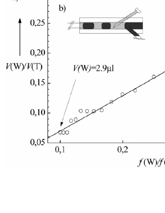
Figure 1: a) Generation of a monodisperse water-toluene mixture using a narrow channel (b). The horizontal axis is the ratio of water/toluene pump rates. The vertical axis is the resulting water droplet/toluene volume ratio. An arrow shows the smallest droplet volume which has been generated via this experimental setup. This minimum droplet size scales with the wall-to-wall separation (channel height).

II.1.2 Preparation of step-gradient surfaces

We use, in this series of experiments, the simplest kind of a wetting gradient, namely a step-wise change in the contact angle. As shown in Fig. 2c, a step gradient consists of two half planes of different wetting properties. It is, therefore, easy to fabricate via partly dip-coating of initially hydrophilic substrates (silicon wafer, glass) with hydrophobic coatings as schematically illustrated in Fig. 2a.

The substrate is dipped into the solution containing the methacrylate copolymer. The substrate is not dipped into a solution of the different components. The methacrylate copolymer contains a silane cross-linking component. This component leads not only to internal cross-linking of the polymer film but also to cross-linking of the substrate by the formation of siloxane bonds.

For the hydrophobic coating, we use the block-co-polymer Poly-(tert-butylmethacrylate-co-Zonyl${}^{\mbox{\textregistered}}$-co-3-trimethoxysilylpropylmethacrylate) 6:2:2 provided by our co-worker R. Frenzel from the IPF Dresden DuPont2002 ; Degischer2003 . The fabrication process is proven to be reproducible and the surfaces show stable wetting properties over long periods of time.

The substrates are characterized by contact angle measurements and ellipsometry. Varying the block-copolymer concentration of the toluene solution and the dip-coating speed, we are able to control the thickness of the coating film in the range of 5nm to 24nm. The wetting properties of the coated substrate are found to be independent of the film thickness with an average advancing contact angle of $105^{\circ}$ and an average receding contact angle of $79^{\circ}$. The polymer films turned out to be stable after exposition to water and solvents for 30 min at $65^{\circ}$C in the ultrasonic bath. The polymer coatings have the advantage to form stable homogeneous films on all substrates of interest such as silicon wafers, glass, aluminum, silicon nitride and epoxy resins.

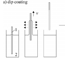
Figure 2: a) Schematic illustration of the dip-coating process: the substrate (1) is dipped into a polymer solution (2). By removing the substrate at a speed $v$ liquid is dragged along with the substrate. The solvent evaporates and the polymer concentration increases until a polymer film forms. b) Schematic view of the thin film structure: After annealing in water vapor, a block-copolymerfilm builds up which consists of a methacrylate bulk, hydrophobic fluoropolymer chains and former crosslinking agent. c) Digital photograph of a silicon substrate, coated with the block-copolymer film on the right half. In the lower picture, water droplets have been sprayed onto the substrate to visualize the wettability step gradient.

II.2 Theoretical method

In parallel to the above mentioned experimental methods, we also address basic questions relevant for the separation process theoretically. This includes simple analytical estimates as well as lattice Boltzmann computer simulations.

In the past twenty years, the lattice Boltzmann method McNamara1988 ; Higuera1989 ; Benzi1992 ; Qian1992 has proved itself as a versatile theoretical tool for the study of a variety of fluid dynamical phenomena such as the flow through porous media Gunstensen1993 , flow of polymer solutions Ahlrichs1999 as well as properties of suspensions of solid particles Ladd2001 , to name just a few examples. Comprehensive introductions to the general foundations of the lattice Boltzmann method can be found in recent monographs Rothman1997 ; Wolf-Gladrow2000 ; Succi2001 as well as in review articles Chen1998 ; Raabe2004 .

While examples given above are mainly based on (extensions of) the LB method for the so called ideal fluids (fluids with an ideal gas equation of state), other LB approaches have been devised allowing the simulation of e.g. a liquid in coexistence with its vapor as well as a binary fluid mixture Shan1993 ; Swift1995 ; Luo1998 .

In this work, we employ a free energy based lattice Boltzmann method capable of adequately simulating both the static and the dynamic properties of a liquid-vapor system. The method has first been proposed by Swift and coworkers who used the method for a study of spinodal decomposition and domain growth Swift1995 . The original version of the method suffered, however, from the lack of Galilean invariance, a serious drawback, when hydrodynamic transport becomes a relevant issue.

This problem was solved by Holdych and coworkers Holdych1998 who proposed a modified expression for the relation between the pressure tensor and the second moments of the population densities in the lattice Boltzmann model. The model was developed further by other coworkers and was applied for a study of interesting issues such as the motion of three phase contact line in two dimensions Briant2002 and roughness effects on liquid-solid slippage Dupuis2006 .

The reader interested in an elaborate discussion of the present lattice Boltzmann approach is referred to many publications by Julia Yeomans and coworkers, some examples of which were cited above Swift1995 ; Holdych1998 ; Briant2002 ; Dupuis2006 . Here, we give a brief overview of the method only.

The starting point of the approach is a free energy functional of the form

$$\Psi=\int_{\Omega}d^{3}r({\psi_{\mathrm{b}}}(\rho({\vec{r}}))+\frac{k}{2}|\vec{\nabla}\rho|^{2})+\int_{S}dS\psi_{\mathrm{s}}.$$ (1)

In Eq. (1), ${\psi_{\mathrm{b}}}(\rho)$ is the free energy per unit volume of a homogeneous system at density $\rho$ and $\psi_{\mathrm{s}}$ the free energy per unit area associated with the presence of the substrate. The first integral extends over the volume of the fluid (containing both the gas and the liquid phases) $\Omega$ and the second integral is evaluated over the surface of the substrate $S$.

In the LB model adopted in the present simulations, the free energy density of the homogeneous phase ${\psi_{\mathrm{b}}}$ is given by Briant2002

$${\psi_{\mathrm{b}}}={p_{\mathrm{c}}}({\nu_{\rho}}+1)^{2}({\nu_{\rho}}^{2}-2{\nu_{\rho}}+3-2\beta{\nu_{T}})$$ (2)

and the resulting equation of state ($p=\rho\partial{\psi_{\mathrm{b}}}/\partial\rho-{\psi_{\mathrm{b}}}$) is Leopoldes2003

$$p={p_{\mathrm{c}}}({\nu_{\rho}}+1)^{2}(3{\nu_{\rho}}^{2}-2{\nu_{\rho}}+1-2\beta{\nu_{T}}).$$ (3)

In Eqs. (2) and (3) ${\nu_{\rho}}=(\rho/{\rho_{\mathrm{c}}}-1)$, ${\nu_{T}}=(1-T/{T_{\mathrm{c}}})$ and ${p_{\mathrm{c}}}=1/8$, ${\rho_{\mathrm{c}}}=7/2$ and ${T_{\mathrm{c}}}=4/7$ are the critical pressure, density and temperature respectively. The parameter $\beta$ is a constant allowing to tune e.g. the temperature dependence of equilibrium densities of the liquid and the vapor phases Briant2002

$$\rho_{\mathrm{L,G}}={\rho_{\mathrm{c}}}\left(1\pm\sqrt{\beta{\nu_{T}}}\right)$$ (4)

with $\beta=0.1$ in our simulations. As shown by Cahn and Hilliard in their seminal work Cahn1958 , within a free energy based model similar to that underlying the present LB approach, the surface tension can be obtained from the knowledge of the density profile as an integral over the density gradient across the liquid-vapor interface (here assumed to be perpendicular to the $z$-axis)

$$\sigma=\kappa\int\left(\frac{\partial\rho}{\partial z}\right)^{2}dz.$$ (5)

Equivalently, given the input parameters of the present LB model, $\sigma$ can also be obtained from the analytic expression Briant2002

$$\sigma=\frac{4{\rho_{\mathrm{c}}}}{3}\sqrt{2\kappa{p_{\mathrm{c}}}}(\beta{\nu_{T}})^{3/2}.$$ (6)

A nice feature of Eqs. (5) and (6) is that they provide an independent way to test the reliability of the simulation results.

In all the simulations to be reported below, we used $T=0.4$ corresponding to ${\nu_{T}}=0.3$. This choice is below the critical temperature and gives rise to a liquid phase in equilibrium with its vapor with corresponding densities of ${\rho_{\mathrm{L}iquid}}\approx 4.1$ and ${\rho_{\mathrm{G}as}}\approx 2.9$. Unless otherwise stated, the LB relaxation time is set to $\tau=0.8$ (Eq. (11)) and a value of $\kappa=0.004$ is used. The geometry of the simulation is a rectangular three dimensional lattice. The topography of the substrate is perfectly planar (no roughness) and parallel to the $xy$-plane. It is placed both at the bottom of the box ($z=0$) and on the top ($z=L_{z}-1$). Periodic boundary conditions are applied along the $x$ and $y$ directions.

In order to save computation time, system size is varied depending on the specific situation with typical values around $L_{x}\times L_{y}\times L_{z}=100\times 100\times 100$.

As to the effect of a substrate on system properties, minimizing the free energy functional $\Psi$ [Eq. (1)] subject to the boundary condition that $\psi_{\mathrm{s}}=-\phi_{1}{\rho_{\mathrm{s}}}$ Cahn1958 ; deGennes2002 , where $\phi_{1}$ is a constant and ${\rho_{\mathrm{s}}}$ the fluid density at the substrate, leads to the condition that the gradient of the density in the direction normal to the substrate (${\vec{s}}$) must satisfy Leopoldes2003

$$\kappa{\vec{s}}\cdot\vec{\nabla}\rho=-\phi_{1}.$$ (7)

Introducing the equilibrium contact angle $\theta$ and assuming a planar substrate at $z=0$ parallel to the $xy$-plane (${\vec{s}}\cdot\vec{\nabla}=\partial/\partial z$), it can be shown that Leopoldes2003

$$\frac{\partial\rho}{\partial z}=-2\beta{\nu_{T}}\sqrt{\frac{2{p_{\mathrm{c}}}}{\kappa}}\mathrm{sign}(\theta-\frac{\pi}{2})\sqrt{\cos(\frac{\alpha}{3})[1-\cos(\frac{\alpha}{3})]}.$$ (8)

The angle $\alpha$ is determined by the input contact angle $\theta$ via $\cos(\alpha)=\sin^{2}(\theta)$. Note that, in contrast to Eq. (7), the dependence of the density gradient on $\phi_{1}$ is no longer explicit. Rather, it affects $\partial\rho/\partial z$ at the substrate via the equilibrium contact angle $\theta$. This is a nice feature allowing the use of $\theta$ as input parameter of the simulation.

Turning our attention to the simulation technique, we now address the central quantity within a lattice Boltzmann scheme, the so called distribution function (or population density) $f_{i}$. Imagine a volume of fluid around a point ${\vec{r}}$ at time $t$ and divide the fluid within this volume to a finite number of portions (parcels). Roughly speaking, $f_{i}({\vec{r}},t)$ would then denote the fluid fraction (parcel) moving with a velocity ${\vec{c}_{i}}$. Obviously, once the populations $f_{i}({\vec{r}},t)$ are known, one obtains the fluid density $\rho$ and velocity ${\vec{u}}$ via

$$\rho({\vec{r}},t) = \sum_{i=0}^{b}f_{i}({\vec{r}},t)$$ (9)

$$\rho({\vec{r}},t){\vec{u}}({\vec{r}},t) = \sum_{i=1}^{b}f_{i}({\vec{r}},t){\vec{c}_{i}},$$ (10)

where we already assumed a regular lattice, where each site is linked to $b$ neighboring sites. Here, the index $i$ is used to enumerate various links ${\vec{c}_{i}}$ along which a lattice node is connected to its neighbors. The reader may have noticed that we do not distinguish between velocity and link vectors. This is a result of the underlying LB scheme, where a fluid portion moving along the link number $i$ travels the whole length of the link during one single time step (this gives rise to a higher speed along diagonal directions compared to the main coordinate directions; see also below).

In the present LB model, we use a regular cubic lattice, where a given node is connected to its neighbor nodes along the 6 coordinate directions ${\vec{c}_{i}}\in\{(\pm 1,0,0),(0,\pm 1,0),(0,0,\pm 1)\}$ ($i=1,...,6$) as well as along the 8 diagonal directions ${\vec{c}_{i}}\in\{(\pm 1,\pm 1,\pm 1)\}$ ($i=7,...,14$). The index $i=0$ is reserved for the null vector, ${\vec{c}}_{0}=\vec{0}$, corresponding to the so called rest particles. This defines to so called three dimensional 15 velocity (D3Q15) LB model.

Within a lattice Boltzmann method, one basically iterates two simple steps generally referred to as (1) relaxation (collision) and (2) free propagation (streaming),

$$f_{i}^{\prime}({\vec{r}},t)=f_{i}({\vec{r}},t)-\frac{1}{\tau}[f_{i}({\vec{r}},t)-{f^{\mathrm{eq}}_{i}}({\vec{r}},t)]$$ (11)

$$f_{i}({\vec{r}}+dt{\vec{c}_{i}},t+dt)=f_{i}^{\prime}({\vec{r}},t),$$ (12)

where we introduced $f_{i}^{\prime}$ in order to formally separate the relaxation and streaming steps. In Eq. (11), the quantity $\tau$ is the so called relaxation time which determines the fluid’s kinematic viscosity, $\nu=\eta/\rho$ ($\eta$=viscosity, $\rho$=fluid density). For the present three dimensional 15 velocity model, one finds Briant2002 $\nu=(\tau-0.5)dx^{2}/(3dt)$, where $dx$ is the distance between two neighboring nodes connected along the main coordinate directions and $dt$ is the time step.

Physical properties of the system enter the LB iteration scheme via the quantity ${f^{\mathrm{eq}}_{i}}$ (Eq. (11)). Obviously, the system is ’pushed’ towards ${f^{\mathrm{eq}}_{i}}$ with a rate $1/\tau$. The population density ${f^{\mathrm{eq}}_{i}}$ is, therefore, referred to as ’equilibrium distribution’. It is noteworthy that the term ’equilibrium’ does not refer to a global thermal equilibrium, where no flow exists. Rather, it describes the local velocity distribution in a portion of fluid moving at a velocity ${\vec{u}}({\vec{r}})$. Within the present LB model, one expands ${f^{\mathrm{eq}}_{i}}$ in powers of the fluid velocity ${\vec{u}}$ up to the second order Briant2002 :

$${f^{\mathrm{eq}}_{i}}=A_{\sigma}+B_{\sigma}{\vec{u}}\cdot{\vec{c}_{i}}+C_{\sigma}u^{2}+D_{\sigma}({\vec{u}}\cdot{\vec{c}_{i}})^{2}+{\vec{c}_{i}}\cdot\tensor{G}_{\sigma}\cdot{\vec{c}_{i}}$$ (13)

for $i>0$. The population of the rest particles then results from the constraint that the relaxation (collision) process does not change the fluid density. This leads to $\sum^{b}_{i=0}{f^{\mathrm{eq}}_{i}}=\sum^{b}_{i=0}f_{i}=\rho$ ($b=14$ for the D3Q15 LB model), whereby leading to

$$f_{0}^{\mathrm{eq}}=\rho-\sum^{b}_{i=1}{f^{\mathrm{eq}}_{i}}.$$ (14)

Note that, even though the fluid density is unchanged during collision, it may undergo a variation through the streaming step. The use of the index $\sigma$ instead of $i$ in Eq. (13) is motivated by the fact that, due to symmetry requirements, we expect exactly the same coefficients for all the links along principal directions, $i=1,...,6$. In other words, $A_{1}=A_{2}=...=A_{6}$, $B_{1}=B_{2}=...=B_{6}$, etc. The value $\sigma=1$ is thus used for $i\in\{1,...,6\}$. Similarly, $\sigma=2$ corresponds to all the links along diagonal directions, reflecting $A_{7}=A_{8}=...=A_{14}$, $B_{7}=B_{8}=...=B_{14}$, etc. A possible choice of the coefficients $A_{\sigma},\;B_{\sigma},\;C_{\sigma},\;D_{\sigma}$ and the tensor $\tensor{G}_{\sigma}$ is (no summation over repeated indices) Briant2002

$$A_{\sigma} = \frac{w_{\sigma}}{c^{2}}\left\{p-\frac{\kappa}{2}||\vec{\nabla}\rho||^{2}-\kappa\rho\Delta\rho+\nu{\vec{u}}\cdot\vec{\nabla}\rho\right\}$$ (15)

$$B_{\sigma} = \frac{w_{\sigma}\rho}{c^{2}},\;\;C_{\sigma}=-\frac{w_{\sigma}\rho}{2c^{2}},\;\;D_{\sigma}=\frac{3w_{\sigma}\rho}{2c^{4}}$$ (16)

$$G_{1\gamma\gamma} = \frac{1}{2c^{4}}\left\{\kappa(\partial_{\gamma}\rho)^{2}+2\nu u_{\gamma}\partial_{\gamma}\rho\right\}$$ (17)

$$G_{2\gamma\gamma} = 0$$ (18)

$$G_{2\gamma\delta} = \frac{1}{16c^{4}}\left\{\kappa(\partial_{\gamma}\rho)(\partial_{\delta}\rho)+\nu(u_{\gamma}\partial_{\delta}\rho+u_{\delta}\partial_{\gamma}\rho)\right\}$$ (19)

$$(\gamma\neq\delta).$$

where Greek letters label Cartesian coordinates $x_{\gamma},x_{\delta}\in\{x,y,z\}$ and $\partial_{\gamma,\delta}\equiv\partial/\partial x_{\gamma,\delta}$. Note that the tensor $\tensor{G}_{1}$ couples to velocities ${\vec{c}_{i}}$ parallel to the coordinates axis ($i=1,...,6$) only. The non-diagonal components of $\tensor{G}_{1}$ are, therefore, of no interest here.

In Eqs. (15)-(19), $w_{1}=1/3$ and $w_{2}=1/24$ are constant weights and $c=\delta x/\delta t$ is the velocity along a principal direction (note that the velocity along a diagonal line is $\sqrt{3}c$). $\kappa$ is a parameter which tunes the width of the liquid-vapor interface and the related surface tension (see also below). In addition to the presence of spatial derivatives of fluid density, non ideal effects are also accounted for in the expression for the pressure $p$ [Eq. (3)] which enters the equilibrium distribution ${f^{\mathrm{eq}}_{i}}$ via the coefficient $A$ [see Eqs. (13) and (15)].

III Results and discussion

In order to obtain a first, order of magnitude, estimate of the driving forces present in the separation process, we give in the next section simple analytical estimates of these forces for the two interesting cases of open substrate and closed planar geometry (slit). Results of experiments as well as lattice Boltzmann simulations will then be presented in the subsequent sections.

III.1 Driving forces of the separation process

In a typical separation experiment, a binary emulsion enters the gradient zone in a direction perpendicular to the direction of wetting gradient (see e.g. the lower image in Fig. 4b). In the absence of a wetting gradient, each component of the emulsion would have equal probabilities of selecting either the right or the left arm of the channel. The role of the wetting gradient is to induce a preferential deflection of at least one of the fluid components.

Note that, as will be shown below (Figs. 5 and 6), selective wetting of one of the fluid components is sufficient for a successful separation. To keep the analysis as simple as possible, it is, therefore, reasonable to first focus on the effects of a step-wise wetting gradient on the motion of a single fluid droplet.

Suppose that a fluid droplet is in contact with both hydrophilic and hydrophobic parts of a substrate with a step-like wetting gradient. Due to different contact angles on the both sides of the wetting gradient, there will be a net force on the droplet pushing it towards the more hydrophilic (or, equivalently, less hydrophobic) part of the substrate. This force is proportional to the derivative of the underlying thermodynamic potential (the sum of all the surface free energies involved in the problem) with respect to the equilibrium contact angle.

On the other hand, it is not unreasonable to assume that the droplet can locally adapt its contact angle to the local equilibrium value within a time short compared to the translation of the droplet over the chemical step. In this case, the droplet shape will be a kind of compromise (interpolation) between two spherical caps, corresponding to the contact angles on both sides of the wettability step. Focusing on the proximity of the substrate, the droplet shape far from the chemical step will be close to that of a spherical cap with a contact angle-dependent radius of curvature. As a consequence, a gradient in the Laplace pressure (see below) will form inside the droplet, trying to push it towards the more hydrophilic side of the substrate (see e.g. Fig. 7).

It is, therefore, instructive to start with simple analytical estimates of the Laplace pressure and its dependence on the contact angle and other relevant parameters.

Let us first consider the case of a droplet forming a spherical cap on a chemically homogeneous open substrate (the panel a) in Fig. 3). For a spherical cap of volume $\Omega$ and static contact angle $\theta$, the pressure inside the droplet is $p=p_{0}+p_{\mathrm{Laplace}}(\theta,\Omega)$, where $p_{0}$ is the pressure outside the droplet, and $p_{\mathrm{Laplace}}=2\sigma/R_{0}$ the so called Laplace pressure arising from the curvature $R_{0}$ of the liquid-vapor interface ($\sigma=$surface tension. The factor of 2 originates from the presence of two equal radii of curvature).

Note that, in the above, we express the pressure inside the droplet in terms of the radius of curvature and not the radius of contact area. The latter being given by $R=R_{0}\sin(\theta)$, one recovers the (perhaps more familiar) expression $p=p_{0}+2\sigma\sin(\theta)/R$.

The radius of curvature of a spherical cap is given by

$$R_{0}=\left(\frac{\Omega}{\pi(2/3+\cos(\theta)^{3}/3-\cos(\theta))}\right)^{1/3}$$ (20)

as can be obtained via integrating a portion of the sphere for polar angles in the interval [0, $\theta$]. Inserting this information into the expression for the Laplace pressure within a spherical cap, we obtain

$$p_{\mathrm{Laplace}}=\frac{2\sigma}{R_{0}}=2\sigma\left(\frac{\pi(2/3+\cos(\theta)^{3}/3-\cos(\theta))}{\Omega}\right)^{1/3}.$$ (21)

The panel c) in Fig. 3 shows, for the case of water, the Laplace pressure versus contact angle for a spherical cap of $\Omega=5\mu$l volume (circles). For contact angles close or below $\theta=90^{\circ}$, the Laplace pressure varies rather fast but then approaches a quasi-plateau as the hydrophobic zone is reached. The horizontal dashed line serves to highlight this limiting behavior.

Note that it is the difference in Laplace pressure, $\delta p=p_{\mathrm{Laplace}}(\theta_{2})-p_{\mathrm{Laplace}}(\theta_{1})$, which is the origin of a driving force. More precisely, for a given variation in the contact angle, the driving force per unit volume (force density), ${\vec{f}^{\mathrm{driv}}_{\mathrm{Laplace}}}$, is proportional to the gradient of the Laplace pressure:

$${\vec{f}^{\mathrm{driv}}_{\mathrm{Laplace}}}=-\vec{\nabla}p_{\mathrm{Laplace}}=-\frac{\partial p_{\mathrm{Laplace}}}{\partial\theta}\vec{\nabla}\theta.$$ (22)

Since ${\partial p_{\mathrm{Laplace}}}/{\partial\theta}$ on open substrates approaches zero for large contact angles, increasing the contact angle of the more hydrophobic part of the substrate (i.e. making it still more hydrophobic) does not necessarily lead to a significantly higher driving force density.

This idea is nicely born out in panel d) of Fig. 3, where we show (for the case of water) the gradient of the Laplace pressure versus droplet volume (see also Eq. (24) below) for the same difference in contact angle $d\theta=\theta_{2}-\theta_{1}=50^{\circ}$ while shifting both $\theta_{1}$ and $\theta_{2}$ towards progressively higher values. Obviously, at constant $d\theta$, the higher $\theta_{1}$ the lower the wettability gradient induced driving force density.

Using Eqs. (21) and (22), we can also estimate the dependence of the wettability induced driving force density on the volume of a spherical cap

$${f^{\mathrm{driv}}_{x,\mathrm{Laplace}}} \simeq -\frac{p_{\mathrm{Laplace}}(\theta_{2})-p_{\mathrm{Laplace}}(\theta_{1})}{l_{x}}$$ (23)

$$\propto \frac{1}{R_{0}^{2}}\propto\frac{1}{\Omega^{2/3}}\;\mbox{(open substrate)}.$$ (24)

In deriving the scaling relation 24, it is assumed that the lateral extension of the droplet (the length $l_{x}$ over which the difference in Laplace pressure builds up) is equal to the sum of the radii of contact, $R_{1}$ and $R_{2}$, corresponding to contact angles $\theta_{1}$ and $\theta_{2}$, respectively:

$$l_{x}\simeq(R_{1}+R_{2})=R_{0}(\theta_{1})\sin(\theta_{1})+R_{0}(\theta_{2})\sin(\theta_{2}).$$ (25)

In contrast to open surfaces, the radius of curvature of the liquid/air front for a liquid film inside a channel made of parallel plates (slit geometry) does not depend on the droplet volume, provided that the liquid volume is large enough to fill the gap vertically and reach a lateral extension larger than the gap height. Moreover, for channel heights smaller than the capillary length, the gravitational effects on the shape of the liquid/air interface may be neglected deGennes2002 .

Under these circumstances, the radius of curvature of the liquid/air front in a planar slit is given by $R_{0}=H/(2\cos(\theta))$. As a consequence, the Laplace pressure within a liquid film enclosed in a planar channel is obtained as

$$p_{\mathrm{Laplace}}=-\frac{2\sigma\cos(\theta)}{H}\;\;\;\;\;(\mbox{slit geometry}).$$ (26)

To make a parallel to Eq. (24) for the case of slit geometry, we estimate the dependence of the resulting wettability induced driving force density on the volume of fluid enclosed in a planar slit. Assuming that the fluid takes the shape of a circular disk, the lateral extension of a droplet of volume $\Omega$ within a narrow slit of height $H$ can be estimated from $\pi r^{2}H=\Omega$. This gives $l_{x}^{\mathrm{slit}}\simeq 2r=\sqrt{4\Omega/(\pi H)}$ and hence

$${f^{\mathrm{driv}}_{x,\mathrm{Laplace}}} \simeq -\frac{p_{\mathrm{Laplace}}(\theta_{2})-p_{\mathrm{Laplace}}(\theta_{1})}{\sqrt{4\Omega/(\pi H)}}$$ (27)

$$\propto \frac{1}{(H\Omega)^{1/2}}\;(\mbox{slit}),$$ (28)

where Eq. (26) for $\delta p_{\mathrm{Laplace}}$ is used. Note that the scaling laws Eqs. (28) and (24) can also be obtained via an estimate of the gradient of surface free energies involved in the process.

Let us examine whether we are allowed to use the above estimates in the case of our experiments. For this purpose we first estimate the capillary length in order to see whether neglecting gravity is justified. For water, using the values of the surface tension $\sigma=0.07\mathrm{N/m}$, mass density $\rho=10^{3}\mathrm{kg/m}^{3}$ and gravitational acceleration $g=9.8\mathrm{m/s}^{2}$, the capillary length can be estimated as $l_{\mathrm{capillary}}=\sqrt{\sigma/g\rho}\approx 2.67$mm. Since the height of the channel used in our experiments is $H=0.5$mm and thus significantly smaller than $l_{\mathrm{capillary}}$ (see Fig. 5), gravity does not play a major role here.

As to the independence of the radius of curvature from the liquid volume, the size of the smallest fluid droplet leaving our emulsion generator is $\Omega\approx 2.9\mu$l (see Fig. 1). Once entered the planar slit, such a droplet spreads horizontally taking approximately the shape of a circular disk (cylinder) with a radius, $r$, given by $\pi r^{2}H\approx\Omega$. Setting the numbers $\Omega=2.9\mathrm{mm}^{3}$ and $H=0.5$mm, one obtains $r\approx 1.36$mm which is roughly three times the gap height. This justifies the assumption that the shape of the liquid-vapor interface is independent of the droplet volume.

Thus, even for the smallest droplet in our experiments, the Laplace pressure within the slit and the corresponding wettability gradient induced driving forces can be estimated via Eqs. (26) and (28).

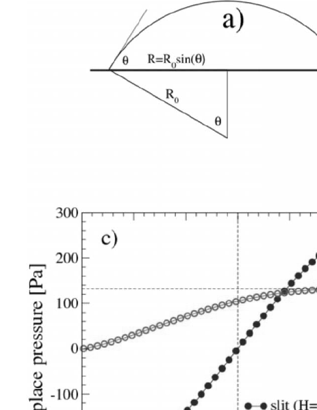
Figure 3: a) and b) Schematic views of a droplet on a chemically homogeneous open substrate [a)] and a liquid film confined in a planar gap with a wetting gradient [b)]. c) The Laplace pressure versus contact angle both for a 5$\mu$l spherical cap of water placed on an open substrate and within a liquid film of water confined in a planar gap of height $H=0.5$mm as indicated. A vertical dashed line marks $\theta=90^{\circ}$. A horizontal dashed line marks the limiting value of the Laplace pressure in the case of spherical cap for $\theta\to 180^{\circ}$. It serves to underline the presence of a plateau in this limit on open substrate. d) The gradient of Laplace pressure versus droplet volume within a spherical cap [Eqs. 21 and 23] and in a planar slit [Eqs. 26 and 27] for a contact angle difference of $d\theta=50^{\circ}$ as indicated. For comparison, a horizontal dashed line marks the gravitational force density. A vertical dashed line marks $\Omega=5\mu$l, for which the $\theta$-dependence of $p_{\mathrm{Laplace}}$ is shown in the panel c).

The dependence of the Laplace pressure upon the contact angle for the case of a closed planar geometry is shown in the panel c) of Fig. 3 for a channel of height $H=0.5$mm as used in our experiments. Obviously, for the range of parameters studied in our experiments, the slit geometry allows the formation of significantly higher gradients in Laplace pressure than would be possible on an open substrate.

Furthermore and in sharp contrast to open geometry, this applies to contact angle variations both in the hydrophilic and in the hydrophobic regime: As shown in the panel d) of Fig. 3, for a difference of $\theta_{2}-\theta_{1}=50^{\circ}$, the curves for $\theta_{1}=55^{\circ}$ and $\theta_{1}=85^{\circ}$ are practically identical in the case of a slit geometry while on open substrate the gradient of the Laplace pressure drops significantly when going from $\theta_{1}=55^{\circ}$ to $\theta_{1}=85^{\circ}$.

A significant decrease of $\nabla p_{\mathrm{Laplace}}$ is, however, observed also in the case of a slit when choosing $\theta_{1}=120^{\circ}$ and $\theta_{2}=170^{\circ}$. This is not surprising since the Laplace pressure as a function of the contact angle gradually flattens for large contact angles. This point is nicely seen in the panel c) of Fig. 3.

While neglecting many complications occurring in real experiments, this simple estimate yields at least a qualitative understanding of higher separation efficiency observed in confined channels as compared to open substrates.

III.2 Separation experiments on step gradients

A variety of separation experiments on surfaces with step gradients have been performed. All these experiments show efficient separation processes with high reproducibility PagraDiss . Additionally, it is possible to vary the flow velocity of the emulsion over a wide range. The efficiency of step gradients is first tested on open substrates using different lateral geometries and wettability contrasts between the hydrophilic and hydrophobic parts of the substrate (Fig. 4).

A demixing of the water-toluene emulsion is observed in all the experiments performed on open substrates. Furthermore, these experiments suggest that the selectivity of water with respect to the both parts of the substrate mainly drives the separation. We will come back to this important point below.

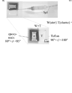
Figure 4: a) Separation of a water-toluene emulsion in a microfluidic cell. The cell is milled into a Teflon block (hydrophobic) with a cavity filled with epoxy resin (hydrophilic). A toluene/water mixture serves as emulsion, where blue ink dissolved into the water is used to enhance the contrast. While toluene wets both surfaces roughly in the same way, water exhibits a strong tendency to selective wetting. (b) Top: A silicon substrate partially coated by a fluorosilane (right half). The uncoated part is strongly hydrophilic (contact angle of 64^∘) while the coated part is hydrophobic (104^∘). Bottom: A separation experiment performed on this substrate.

With respect to applications, experiments in confined geometries are of major importance because confinement prevents fast liquid evaporation that would occur in open miniaturized systems. Therefore, in a further step, we turned our attention to separation experiments in confined geometries, i.e. in closed cells.

Separation cells with widths (horizontal extensions) of 1mm, 2mm, 3mm, 4mm, 8mm, 14mm and 20mm were used. However, for the separation cells with a width less than 20mm, a stable reproducible separation process could not be established. Qualitatively, we observe a decrease of separation efficiency upon a reduction of channel width. This suggests that adhesive forces due to surface energy hysteresis oppose the driving forces induced by the step gradient of wettability. A detailed analysis of this issue can be found in PagraDiss .

In the case of the largest separation cell investigated (width=20mm), the separation efficiency is 100% for flow rates up to 2 ml/min and no ’mislead’ droplets are observed. For flow rates between 5 ml/min and 10 ml/min single droplets of the ’wrong’ component are observed on the hydrophobic and the hydrophilic side. The estimated separation efficiency in this case remains well above 90%. Currently, a separation cell with integrated reservoirs for each outlet is being developed which will enable us to specify the separation efficiency more precisely. However, this modification is not trivial because the attachment of additional fluidic components changes the boundary conditions of the whole problem.

Figure 5 shows a digital photograph of the separation chamber. It consists of an aluminum block (1) into which a planar channel has been milled (with a tiny hole in the middle that serves as the inlet). The aluminum channel is covered by a glass substrate (2) which is glued onto the aluminum block by epoxy resin (3). The aluminum and the glass part are both half-coated with the block-copolymer film. The dimensions of the so constructed channel are $L=75$mm (length), $W$=20mm (width) and $H=0.5$mm (height).

At early stages of the separation (a), water (W) exclusively wets the hydrophilic side. Interestingly, the non-polar component of the mixture (here hexane (H)) also shows a tendency to flow along with water and wets the hydrophilic part of the channel (see the liquid/air front in Fig. 5a. However, the situation changes as soon as water reaches both sidewalls. At this point, the water front formed across the channel hinders the motion of the non-polar component towards the hydrophilic side. The latter thus flows towards the hydrophobic side and the separation becomes perfect (Fig. 5b).

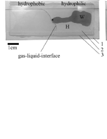
Figure 5: W=Water, H=Hexan, 1=Aluminum channel 2=Glass cover, 3=Clay (Epoxid). The left halves of both the Aluminum channel and the glass cover are covered with a hydrophobic coating (fluoropolymer). (a) Initial stage of separation. (b) Final state. The channel has a length of $L=75$mm, a width of $W$=20mm and a vertical dimension of $H=0.5$mm.

III.2.1 The effect of a secondary flow on separation efficiency

Motivated by the above discussed observation, that the separation becomes practically perfect as soon as the water component reaches both side walls, we introduce an additional water source in order to enhance the separation efficiency. Figure 6 shows a digital photograph of a separation chamber designed for this purpose. The chamber has two inlets. Through the one inlet the hexane-water-mixture is introduced, whereas through the other inlet only water is injected. For visualization purpose, the water component in the mixture is colored with ink. As soon as the two water components come into contact, they form a continuous front across the channel pushing hexane to the right side of the channel.

At later stages of flow separation, a sharp interface builds up between the hexane and the aqueous phase. The straight interface between the two water components (indicated as W and W2) reflects the laminar nature of the flow, a characteristic feature of most (but not all, see e.g. Varnik2006a ; Varnik2007a ; Varnik2007b ) microflows. Due to the absence of chaotic behavior, the two water components mix via diffusion only, a process slow compared to the time scale of the separation experiment.

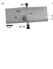
Figure 6: W=Water with ink, H=Hexane, W2=Water as secondary flow, 1=Glass cover, 2=Sidewalls made of epoxy resin. Sidewalls, glass cover and the bottom substrate are half coated with the hydrophobic block-copolymer film. (a) separation starts as soon as both water components W and W2 meet. (b) nearly perfect separation result.

III.3 Lattice Boltzmann simulations

III.3.1 Simulation of wetting gradient driven fluid motion

In section III.1 we addressed, via simple analytic arguments, the driving forces resulting from a change in wetting properties of the substrate. These estimates are, however, based on the assumption of perfect spherical caps on each side of the step gradient with respective contact angles. Obviously, a single droplet covering both sides of a step gradient can not satisfy this condition. Rather, it will try to take a shape consistent with variable wettability of the substrate. This shape will probably resemble to a portion of a spherical cap at each end of the droplet (away from the interface between the hydrophilic and hydrophobic parts of the substrate) with a transition between the two different ’spherical caps’ in the step gradient zone. Furthermore, dynamic effects, such as effects of dissipation loss on the force balance, are fully absent in the above analysis.

This underlines the need for a full theoretical treatment of the problem including the whole complexity of the droplet shape variation across the transition zone as well as the internal fluid dynamics. The lattice Boltzmann simulations to be presented below provide such an approach.

III.3.2 Droplet movement on step-gradients

As already mentioned, a wetting gradient breaks the symmetry of the problem introducing a preferential deflection of a water droplet towards the more hydrophilic side of the channel.

In order to elucidate this issue, we first performed a series of lattice Boltzmann computer simulations of the droplet motion on a step gradient in the absence of external forces. For this purpose, a spherical fluid droplet is deposited at time $t=0$ on the top of a step-like wetting gradient in a way that it slightly touches the line separating the zones of different wettability. The initial velocity of the droplet is zero, so that all dynamic effects originate from the tendency of the liquid to wet the substrate. Furthermore, both the hydrophilic and the hydrophobic halves of the substrate are chosen to be perfectly flat thus ensuring the absence of hysteresis effects. They differ only in their static contact angles with respect to the fluid.

A typical result of these simulations is illustrated in Fig. 7 for a choice of static contact angles $\theta_{1}=75^{\circ}$ (right half) and $\theta_{2}=105^{\circ}$ (left half). Not unexpectedly, the droplet preferentially wets the hydrophilic part of the substrate as illustrated by a sequence of images in Fig. 7. This leads to an asymmetric shape during the spreading process and a net horizontal momentum of the droplet’s center of mass towards the hydrophilic part. This horizontal motion stops as soon as the droplet fully leaves the hydrophobic part of the substrate indicating that inertial effects are negligible in the case studied here.

At this stage, it is instructive to estimate the average time $\bar{t}=l_{x}/(2u)$ ($u$ is the velocity scale and $l_{x}$ the lateral extension of the droplet on the substrate, see Eq. (25)) for the motion of the droplet over the step gradient. For this purpose, we recall that inertial effects are negligible in our simulations. Equating the viscous dissipation $\eta\Delta u$ to the gradient of the Laplace pressure $\nabla p_{\mathrm{Laplace}}$, we can then obtain an estimate of the velocity scale $u$ if we realize that both $u$ and the Laplace pressure $p_{\mathrm{Laplace}}$ vary over the same length scale, $l_{x}$. Thus, $\Delta u\simeq u/l_{x}^{2}$ and $\nabla p_{\mathrm{Laplace}}\simeq[p_{\mathrm{Laplace}}(\theta_{2})-p_{\mathrm{Laplace}}(\theta_{1})]/l_{x}$ (recall that the latter relation has also been used in deriving the scaling relation 24). Along with Eq. (21), this yields

$$u\simeq u_{\mathrm{capillary}}l_{x}[1/R_{0}(\theta_{2})-1/R_{0}(\theta_{1})],$$ (29)

where we used the definition of the capillary velocity $u_{\mathrm{capillary}}=\sigma/\eta$. Introducing a closely related capillarity time, $t_{\mathrm{capillary}}=l_{x}/(2u_{\mathrm{capillary}})$ allows to write

$$\bar{t}\simeq t_{\mathrm{capillary}}\frac{1}{l_{x}[1/R_{0}(\theta_{2})-1/R_{0}(\theta_{1})]}.$$ (30)

Let us estimate the characteristic velocity, $u_{\mathrm{capillary}}=\sigma/\eta$, and the characteristic time, $t_{\mathrm{capillary}}$ for the case shown in Fig. 7. For this purpose, we first estimate the surface tension. Within the present lattice Boltzmann model and for the specific choice of the parameters used in these simulations (here: $\kappa=0.002$) we obtain via Eq. (6) $\sigma\approx 5.42\times 10^{-4}$ (note that all simulated quantities are measured in LB units. In particular, the lattice spacing, $\delta x\equiv 1$, and the LB time unit, $\delta t\equiv 1$).

It is worth noting that an estimate of the surface tension via the integral over the density gradient across the liquid-vapor interface [Eq. (5)] leads to $\sigma\approx 5.47\times 10^{-4}$ (LB units) which is identical to the exact value within an error of $1\%$.

As to the shear viscosity, it is estimated by inserting $\tau=0.8$ and ${\rho_{\mathrm{L}iquid}}\approx 4.1$ into the relation $\eta=\rho\nu=\rho(\tau-0.5)/3$ which gives $\eta\approx 0.41$ in LB units.

Using the above results on the surface tension and the droplet viscosity, the capillary velocity is estimated via $u_{\mathrm{capillary}}=\sigma/\eta\approx 1.32\times 10^{-3}$ (LB units) leading to a capillary time of $t_{\mathrm{capillary}}\approx 2.2\times 10^{4}$, where we used $l_{x}\approx 58$ as obtained via Eq. (25) for a droplet of volume $\Omega=4\pi r_{0}^{3}/3$ with $r_{0}=30$ LB units (see Fig. 7) on a step gradient substrate with contact angles $\theta_{1}=75^{\circ}$ and $\theta_{2}=105^{\circ}$ . Finally, using this value of $l_{x}$ along with Eq. (20) we are able to evaluate Eq. (30) in order to obtain $\bar{t}\approx 2.5t_{\mathrm{capillary}}$.

As simulation results presented in Fig. 7 clearly demonstrate, this rough estimate does indeed yield the correct time scale for the separation process over a step-wise wettability gradient. Thus, in addition to the fact that LB simulation results shown in Fig. 7 are in qualitative agreement with experimental observations of a preferential liquid motion induced by a step-wise change in the wetting properties of the substrate (Figs. 4-6), they also provide a means to address issues related to the separation process in a more quantitative way.

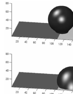
Figure 7: Lattice Boltzmann simulation results on the spreading of a droplet on a step gradient. The left and right parts of the substrate are characterized by static contact angles of $105^{\circ}$ (dark; red online) and $75^{\circ}$ (light (grey online)) respectively. At time $t=0$, a droplet of radius $r_{0}=30$ LB units is positioned on the top of a step gradient slightly touching the substrate (left). As time proceeds, the droplet develops a lateral motion towards the more hydrophilic side. The last image on the right corresponds to the final (equilibrium) state with zero velocity. From left to right: $t=1000,\;4\times 10^{4},\;1.2\times 10^{5},3\times 10^{5}$. After an initial spreading time of approximately $4\times 10^{4}$ LB units, it takes roughly a time of $\bar{t}=8\times 10^{4}\approx 3.6t_{\mathrm{capillary}}$ for the passage of the droplet over the step gradient.

Recalling the discussion of forces driving the motion of a spherical cap on an open substrate (panel d) in Fig. 3), we expect a slower separation dynamics for the same difference in contact angle in the hydrophobic regime. In order to examine this expectation, we performed lattice Boltzmann simulations for the same difference of contact angles $\theta_{2}-\theta_{1}=30^{\circ}$, but in the more hydrophobic regime by choosing $\theta_{1}=105^{\circ}$ and $\theta_{2}=135^{\circ}$ (while keeping all other parameters of the simulation such as the droplet size, the system size, etc. unchanged). In agreement with our qualitative estimate, the time necessary for the transfer of the whole droplet to the hydrophilic part is significantly larger than for the case discussed in the context of Fig. 7.

An important feature of computer simulation of fluid dynamical problems is that not only one has access to the system density at each point in space but also the whole velocity field is known. This is an interesting property since it allows a survey of the liquid motion inside the droplet, whereby providing a means to estimate the viscous dissipation. The latter, in turn, plays a crucial role in determining the droplet dynamics.

Figure 8 shows an example of this strength of computer simulations. The left part of the figure illustrates a projection of the velocity field onto the $xz$-plane for the case studied in Fig. 7 at a time of $t=10^{4}$ (LB unit) corresponding to $\hat{t}\equiv t/t_{\mathrm{capillary}}\approx 0.45$ (recall that $t_{\mathrm{capillary}}\approx 2.2\times 10^{4}$ for the present choice of parameters).

In order to distinguish internal fluid velocity from the velocity of the vapor phase, we also depict the liquid-vapor interface in Fig. 8. This allows to recognize that the fastest lateral motion occurs close to, but not exactly at, the three phase contact line. During droplet spreading, the liquid-vapor interface close to the hydrophilic substrate moves towards right. Quite similarly but with a smaller magnitude, the liquid-vapor interface close to the hydrophobic substrate moves towards left.

As a result of this asymmetric motion, the droplet spreads over the substrate while at the same time its center of mass is shifted towards the more hydrophilic part of the substrate.

Obviously, the observed horizontal motion of the droplet’s center of mass is a result of the presence of a step gradient as highlighted via a comparison to droplet spreading on a chemically homogeneous substrate (i.e. a substrate with a spatially constant contact angle; see the right panel of Fig. 8). In this case, the droplet symmetrically spreads on the substrate in order to reach its static contact angle, the latter being an input parameter of the simulation.

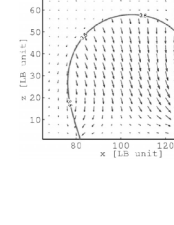
Figure 8: Left: The velocity field within a $xz$-plane at $y=L_{y}/2$ during the spreading of a droplet on a substrate with a step-wise change in contact angle (changing from $\theta=105^{\circ}$ for $x<105$ to $\theta=75^{\circ}$ for $x\geq 105$). The solid line is the liquid-vapor interface (the location of all points with a density equal to $(\rho_{\mathrm{gas}}+\rho_{\mathrm{liquid}})/2$). Obviously, the presence of wetting gradient gives rise to an asymmetric velocity distribution within the droplet. Right: A similar plot but for a droplet spreading on a chemically homogeneous substrate (static contact angle $\theta=60^{\circ}$ for all $x$). As expected, both the shape of the liquid-vapor interface and the velocity field inside the droplet are symmetric. All the snapshots correspond to a time of $t=10^{4}\approx 0.45t_{\mathrm{capillary}}$ after deposing a spherical droplet of radius $r_{0}=30$ lattice units on the substrate.

III.3.3 Competitive effects of wetting gradient and flow pressure: The effect of droplet size

The above lattice Boltzmann simulations address the behavior of a droplet on a step gradient in the absence of flow, thus allowing to focus on the effect of a step gradient alone. When flow is present, there will be a possibility for an accidental deflection of the polar component of the mixture (water in our experiments) towards the more hydrophobic (’wrong’) side. This may be caused e.g. due to imperfect geometry of the channel giving rise to random fluctuations in the velocity field.

As the deflected droplet moves over the step gradient (towards the more hydrophobic side), a gradient of Laplace pressure is formed inside the droplet pushing it back to the more hydrophilic part of the substrate. In order for the separation process to be successful, this wetting gradient induced force must overcome the forces driving the flow. In a two component system, this force is usually the ’flow pressure’. Since our simulation studies are restricted to a one-component fluid and its vapor, we ’mimic’ the flow pressure via an external gravity-like force.

Therefore, it is useful to consider what happens if a droplet is not only subject to the effects of separation forces stemming from the wetting gradient, but also to an opposite force. Figure 9 is devoted to such a situation. To simplify the matter, the flow pressure is mimicked by an external, gravity-like force density. Each row in Fig. 9 illustrates a spherical cap pushed under the action of exactly the same force density towards a chemical step (from hydrophilic part towards hydrophobic one). As the droplet reaches the chemical step, the corresponding gradient in Laplace pressure tries to hinder its motion and to keep it on the more hydrophilic side.

Despite the fact that the both droplets are subject to exactly the same force density, the presence of a wetting gradient leads to quite different dynamic behavior depending on the droplet size. While the larger droplet passes under the action of the external force over the step gradient (upper images in Fig. 9), the smaller one is stopped at the boundary between the hydrophilic and hydrophobic parts of the substrate (lower images).

Following Eq. (24), this observation can be rationalized as follows. The wettability gradient induced force scales as $1/\Omega^{2/3}$ and thus as $1/r_{0}^{2}$, where $r_{0}$ is the radius of the initial droplet on the substrate. Indeed, the two droplets in Fig. 9 differ by a factor of 2 in their initial radii. The force opposing the droplet motion is, therefore, expected to be by a factor of 4 larger in the case of the smaller droplet as compared to the larger one.

As a first test of the scaling behavior given in Eq. (24), we increased the external gravity-like force by a factor of four in order to see whether the smaller droplet is pushed over the step gradient zone in a way similar to the motion of the larger droplet. This naive expectation is, however, not confirmed via our simulations. Nevertheless, an increase of the external gravity like force by a factor of 5 turns out to be sufficient for overcoming the step gradient effects.

Noting that the derivation of Eq. (24) is based on a fully static argument (setting the fluid velocity ${\vec{u}}=\vec{0}$ in the Navier-Stokes equation), the observed deviation between the dynamic behavior and this estimate is not surprising. Rather, it emphasizes the fact that a more quantitative analysis must involve the dynamics of the fluid within the droplet and the corresponding dissipation losses. We are currently working on such a more elaborate analysis.

It is instructive to also discuss various stages of droplet motion for the case of a droplet being pushed over the step gradient zone. Figure 10 shows the center of mass velocity of a fluid droplet on a substrate consisting of a hydrophilic and a hydrophobic part under the action of a gravity-like force. At time $t=0$, a hemisphere of initial radius $r_{0}=40$ (LB units) is placed on the hydrophilic part of the substrate and a gravity-like force density of $g=10^{-6}$(LB units) is switched on.

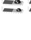
Figure 9: Top: At time $t=0$, a hemisphere of radius $r_{0}=40$ (LB units) is placed on the hydrophilic (light (grey online); static contact angle $\theta=75^{\circ}$) part of a substrate and a gravity-like force of $g=10^{-7}$ (LB units) is switched on pushing the droplet towards the hydrophobic part (dark (red online); $\theta=105^{\circ}$). The time increases from left to right as $t=0,\;3\times 10^{3},\;10^{6},\;2.7\times 10^{6}$ (LB units). Bottom: The same situation as in the upper panels, but for a smaller droplet of $r_{0}=20$ LB units. In this case, gradient of Laplace pressure over the chemical step is strong enough in order to fully stop the droplet motion (from left to right: $t=0,\;2\times 10^{5},\;5\times 10^{5},\;1.5\times 10^{6}$).

The lateral extension of the hydrophilic side of the substrate is chosen such that the droplet can reach its steady state motion before arriving at the interface between the hydrophilic and hydrophobic parts of the substrate (first plateau in the velocity in Fig. 10). At the wettability step, the droplet velocity decreases indicative of additional (wetting gradient induced) forces opposing its motion. The droplet velocity reaches a minimum and then increases again towards a new plateau corresponding to steady state motion on the hydrophobic part of the substrate.

Note that, in agreement with various experimental observations as well as computer simulations Barrat1999 , we observe a higher steady state droplet velocity over a hydrophobic substrate as compared to the hydrophilic one under the action of exactly the same external force. This is indicative of lower dissipation losses for a motion on hydrophobic substrates.

As a consequence of the periodic boundary condition present in our simulations, we can also survey what happens when the external driving and wetting gradient forces act along the same direction. This occurs as the droplet leaves the channel at the left boundary and reenters it from the right side, thereby leaving the hydrophobic substrate towards the hydrophilic one. In this case, the droplet motion is accelerated by the action of the wetting gradient (see the maximum in Fig. 10). Finally, as the gradient zone is left behind, the droplet decelerates to reach its steady state velocity on the hydrophilic substrate.

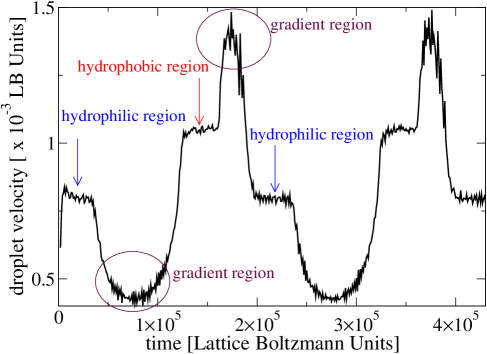
Figure 10: (Color online) Different stages during the motion of a fluid droplet (hemisphere) of radius $r_{0}=20$ lattice units under the action of an external force density of $g=10^{-6}$ (LB units) on an open substrate made of a periodic array of hydrophilic (light (grey online); $\theta=75^{\circ}$) and hydrophobic (dark (red online); $\theta=105^{\circ}$) parts. The system size is $160\times 80\times 40$ (along $x$, $y$ and $z$-directions). Other parameters of the simulation are $\tau=0.8$, $\kappa=0.002$ and $T=0.4$.

Different stages of the droplet motion over a step gradient are also illustrated in Fig. 11 for a smaller droplet (radius $r_{0}=20$ lattice units) moving under the action of a driving force of $g=10^{-6}$ [LB units]. In this figure, we focus on the droplet shape and its variation as the droplet passes over the wettability step. As expected, the droplet spreads better on the hydrophilic part of the substrate than on the hydrophobic part. As a consequence, its lateral extension decreases leading to an increase in its height during the passage over the step gradient zone (moving from right to left).

Note that the shape of a droplet moving on a substrate depends on its velocity. A constant droplet shape may, therefore, give a hint on the presence of a steady state motion. Keeping this in mind, a closer look at regions sufficiently far from the wetting gradient zone in Fig. 11 points to such a steady state motion on both hydrophilic and hydrophobic parts of the substrate. A survey of the velocity versus time (similar to that shown in Fig. 10) confirms this observation.

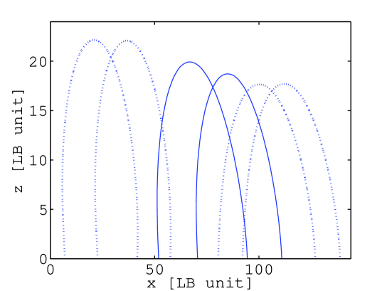
Figure 11: (Color online) A cut along the $xz$-plane of the liquid-vapor phase boundary at $y=L_{y}/2=40$ for a spherical cap of initial radius $r_{0}=20$ (LB units). The interface line is shown at different times during the motion of the spherical cap upon the action of a gravity-like force density of $g=10^{-6}$ (10 times larger than the force applied in the case of Fig. 9). The time increases from right to left as $t=2,\;3.5,\;6,\;10,\;14,\;15.5$ [$\times 10^{4}$ LB units]. The dotted lines correspond to the steady state motion on the hydrophilic (right) and hydrophobic (left) parts of the substrate, whereas the solid lines correspond to the transition over the wettability step (placed at $x=L_{x}/2=80$).

We also studied the competing effects of a wetting gradient and an external driving force in the case of a slit geometry (Fig. 12). Here, we focus on the effect of channel height on the force balance. For this purpose, all parameters of the simulation are kept exactly the same. Only the vertical separation between the substrates is varied. Note that, since we keep the lateral extension of the fluid inside the slit constant, the wettability induced driving force varies as ${f^{\mathrm{driv}}_{x,\mathrm{Laplace}}}\propto\delta p_{\mathrm{Laplace}}/l_{x}\propto\delta p_{\mathrm{Laplace}}\propto 1/H$, where Eq. (26) for $p_{\mathrm{Laplace}}$ in a planar slit is used. As shown in Fig. 12, our simulation results are, at least qualitatively, in line with the expected reduction of ${f^{\mathrm{driv}}_{x,\mathrm{Laplace}}}$ upon an increase of the channel height.

Figure 12: Top: Snapshots of a fluid film in a planar slit of height $H=50$ (LB units) as it is pushed by the action of an external gravity-like force towards left, passing thereby from the hydrophilic (gray; static contact angle $\theta=75^{\circ}$) part of the substrate to the hydrophobic part (dark (red online); $\theta=105^{\circ}$). At time $t=0$ (the image on the left), the space delimited by the two planar interfaces is filled with liquid (for clarity, not the liquid but only the liquid/vapor interfaces are shown). The other three panels correspond to (from left to right) the steady state motion over the hydrophilic substrate ($t=10^{4}$), motion over the step gradient ($t=4\times 10^{4}$) and the steady state motion over the hydrophobic part of the substrate ($t=6\times 10^{4}$). Bottom: The same situation as in the upper panels, but for a smaller channel height of $H=20$ (LB units). In this case, wetting gradient induced forces are strong enough in order to fully stop the fluid motion (from left to right $t=0,\;5\times 10^{4},\;2\times 10^{5},\;5\times 10^{5}$). In the both studied cases, the external force density is $g=10^{-6}$ (LB units).

IV Summary and Conclusion

Basic aspects related to the wetting gradient induced separation of a binary emulsion into its individual components are studied via experiments as well as lattice Boltzmann computer simulations. For the purpose of experimental investigations, an emulsion generator is designed allowing the production of quasi-monodisperse emulsions with well controlled droplet sizes (Fig. 1).

As to the wetting gradient, a step-like change in wetting properties of the substrate is realized via dip-coating process (Fig. 2). Compared to a substrate with a continuous change in wetting properties, the step-like gradients have the advantage of e.g. easy fabrication and long time storage possibility allowing their use up to many weeks after fabrication. Basic results of our separation experiments can be summarized as follows.

It is observed that separation in confined geometry is far more enhanced than on open substrates. Furthermore, the separation process is mainly driven by the selectivity of the water component, i.e. by the tendency of water to preferentially wet the more hydrophilic side of the substrate. This is best seen in a closed channel: Once water fills the whole cross section of the separation chamber, it pushes the other component of the mixture (toluene or hexane in our experiments) to the less hydrophilic part of the channel (Fig. 5).

This property is then used in order to enhance the separation efficiency. For this purpose, a second inlet is introduced on the opposite side of the channel through which water is injected into the separation chamber (Fig. 6). The separation starts as soon as the two water streams meet in the gap and build a water front spanning the whole cross section of the channel.

These experimental observations are accompanied with order of magnitude estimates of the dominant forces responsible for separation [Eqs. (21)-(28) and Fig. 3]. Even though neglecting many complexities present in the real problem, these estimates provide at least a qualitative understanding of the significantly different behavior of wettability induced forces upon a variation of the contact angle in a narrow slit as compared to open substrates.

The analytic estimates given in section III.1 are in qualitative agreement with lattice Boltzmann computer simulations (section III.3). In particular, on open substrate, a stronger gradient in Laplace pressure is observed for the same difference in contact angle in the hydrophilic regime rather than in the hydrophobic one. Such an effect is fully absent in the case of a planar slit, since the dependence of $p_{\mathrm{Laplace}}$ on the contact angle is symmetric upon a variation of $\theta$ around $\theta=90^{\circ}$ [Fig. 3].

Using lattice Boltzmann simulations, we also investigate the effect of a step-like wetting gradient on the motion of a droplet placed at the gradient zone in the absence of flow (Figs. 7 and 8). These simulations confirm that a single step-wise change in the contact angle is sufficient in order to induce a preferential deflection of the droplet towards the region of lower contact angle (Fig. 7).

Via simple scaling arguments we also give an approximate expression for the characteristic time, $\bar{t}$, for the passage of a droplet over the wettability step in the absence of external forces. This time scale turns out to depend on the capillary time, the initial droplet volume as well as on the static contact angles of the hydrophilic and hydrophobic parts of the substrate [Eq. (30)]. Lattice Boltzmann simulations show that the expression given in Eq. (30) yields the correct order of magnitude estimate of $\bar{t}$.

Moreover, a study of the internal fluid dynamics yields interesting insight on how the fluid redistributes within the droplet in order to accommodate both the spreading dynamics and the lateral motion of the droplet towards the more hydrophilic part (Fig. 8).

It would be interesting to examine these computer simulation results in the light of experimental observations. Owning to considerable difficulties in the observation of the local fluid motion, such experiments have not been available yet. Nevertheless, we are planing the use of tracers for visualization purpose and high speed cameras allowing to resolve the fast spreading dynamics of a fluid droplet on a step gradient.

Furthermore, the important role of droplet size as well as channel dimension for the separation process is underlined via analytic estimates [Eqs. (21)-(28)] and computer simulations [Figs. 9 and 12]. While the motion of smaller droplets is dominated by the action of wetting gradient induced forces, larger droplets tend to follow the external gravity-like force [Fig. 9]. A similar effect occurs in the case of a narrow slit (Fig. 12). Here, the effect of wetting gradient induced forces is weakened by an increase of the channel height (vertical separation between the substrates) thus further emphasizing the importance of surface/volume ratio for the separation efficiency.

An important conclusion of our studies is that, both on open substrates and in closed planar channels, larger droplets are harder to guide by a step-wise wetting gradient than are the smaller ones. In the both studied geometries, the wetting gradient induced force decreases with droplet volume $\Omega$ (scaling as $1/\Omega^{2/3}$ on open substrates and as $1/(H\Omega)^{1/2}$ in a planar slit; $H$= channel height).

Since the smallest droplet size is controlled by the dimensions of the emulsion generator (see e.g. Fig. 1) as well as by the height of the planar slit, these observations suggest that a miniaturization of the channel would allow the generation and use of smaller droplets and thus could lead to a significant improvement of the separation efficiency.

Even though of a rather qualitative nature, results presented in this report shed light to some of the basic issues related to the separation phenomena, whereby allowing to isolate interesting aspects for a more quantitative analysis. Such an investigation is the subject of ongoing work.

Acknowledgments

This project was supported by the German Research Foundation (DFG) within the priority program SPP1164, Nano-and Microfluidics, project numbers Va205/3-2 and Sta324/27-2. FV thanks N. Peranio for his assistance during the preparation of this manuscript and A. Dupuis for providing the 3D LB code, which we thoroughly tested and slightly modified for our own purposes.

References

- (1) R. S. Faibish, and Y. Cohen, “Fouling and Rejection Behavior of Ceramic and Polymer-Modified Ceramic Membranes”, Colloids and Surfaces A, 191, 2740 (2001).
- (2) J. K. Holt, H. G. Park, Y. Wang, M. Stadermann, A. B. Artyukhin, C. P. Grigoropoulos, A. Noy, and O. Bakajin, “Fast Mass Transport Through Sub-2-Nanometer Carbon Nanotubes”, Science 312, 1034 (2006).
- (3) T. Gu, ”Liquid-liquid partitioning methods for bioseparations” in Handbook of Bioseparations, volume 2, chapter 7, p 329–364 (Ed. A. Ahuja Academic Press, New York, 2000); T. Gu und L. Zhang, “ Partition Coefficients of Some Antibiotics, Peptides and Amino Acids in Liquid-Liquid Partitioning of the Acetonitrile-Water System at Subzero Temperatures”, Chem. Eng. Comm. 194, 828 (2007).
- (4) S. A. Khan, A. Günther, M. A. Schmidt, K. F. Jensen, “Microfluidic Synthesis of Colloidal Silica”, Langmuir 20, 8604 (2004).
- (5) M. J. Fuerstman, P. Garstecki, G. M. Whitesides, ”Coding/Decoding and Reversibility of Droplet Trains in Microfluidic Networks”, Science 315, 828 (2007).
- (6) M. Prakash und N. Gershenfeld, ”Microfluidic Bubble Logic”, Science 315, 832 (2007).
- (7) A. Günther, S. A. Khan, M. Thalmann, F. Trachsel, K. F. Jensen, “Transport and Reaction in Microscale Segmented Gas Liquid Flow”, Lab Chip 4, 278 (2004).
- (8) B. Zhao, J. S. Moore, D. J. Beebe, “Surface-Directed Liquid Flow Inside Microchannels”, Science 291, 1023 (2001).
- (9) K. Ichimura, S.-K. Oh, M. Nakagawa, “Light-Driven Motion of Liquids on a Photoresponsive Surface”, Science 288, 1624 (2000).
- (10) R. Yamada, H. Tada, “Manipulation of Droplets by Dynamically Controlled Wetting Gradients”, Langmuir 21, 4254 (2005).
- (11) S.-W. Lee, P. E. Laibinis, “Directed Movement of Liquids on Patterned Surfaces Using Noncovalent Molecular Adsorption”, J. Am. Chem. Soc. 122, 5395 (2000).
- (12) L. Ionov, N. Houbenov, A. Sidorenko, M. Stamm, S. Minko, “Smart Microfluidic Channels”, Adv. Funct. Mater. 16, 1153 (2006).
- (13) DuPont™ Zonyl, product data sheet, 2002, E. I. du Pont de Nemours and Company, http://www2.dupont.com/Zonyl_Foraperle/en_US/products/zonyl_pgs/zonyl.html.
- (14) H.-P. Degischer, R. Frenzel, S. Schmidt, V. Hein, M. Thieme, F. Simon, “Ultrahydrophobe Aluminiumoxidoberflächen durch Texturierung und organische Beschichtungen”, Verbundwerkstoffe - 14. Symposium Verbundwerkstoffe und Werkstoffverbunde (2003, Wiley- VCH Verlag, Weinheim).
- (15) G. McNamara and G. Zanetti, “Use of Boltzmann equation to simulate lattice-gas automata”, Phys. Rev. Lett. 61, 2332 (1988).
- (16) F. J. Higuera and J. Jimenez, “Boltzmann Approach to Lattice-Gas Simulations”, Europhysics letters 9, 663 (1989); F. J. Higuera, S. Succi, and R. Benzi, “Lattice gas dynamics with enhanced collisions”, Europhys. Lett. 9, 345 (1989).
- (17) R. Benzi, S. Succi, and M. Vergassola, ”The Lattice-Boltzmann Equation - Theory and Applications”, Phys. Rep. 222, 145 (1992).
- (18) Y. Qian, D. d’Humieres, and P. Lallemand, ”Lattice BGK models for Navier-Stokes equation”, Europhys. Lett. 17, 479 (1992).
- (19) A. Gunstensen and D. Rothman, ”Lattice-Boltzmann studies of two-phase flow through porous media”, J. Geophys. Res. 98, 6431 (1993).
- (20) P. Ahlrichs and B. Dünweg, ”Simulation of a single polymer chain in solution by combining lattice Boltzmann with molecular dynamics”, J. Chem. Phys. 111, 8228 (1999).
- (21) A. Ladd and R. Verberg, ”Lattice-Boltzmann Simulations of Particle-Fluid Suspensions”, J. Stat. Phys. 104, 1191 (2001).
- (22) D. Rothman and S. Zaleski, Lattice-Gas Cellular Automata (Simple Models of Complex Hydrodynamics) (Cambridge University Press, Cambridge, 1997).
- (23) D. Wolf-Gladrow, Lattice-Gas Cellular Automata and Lattice Boltzmann Models (Springer, Berlin Heidelberg, 2000).
- (24) S. Succi, The Lattice Boltzmann Equation for Fluid Dynamics and Beyond (Oxford University Press, Oxford, 2001).
- (25) D. Raabe, ”Overview of the lattice Boltzmann method for nano- and microscale fluid dynamics in materials science and engineering”, Modelling Simul. Mater. Sci. Eng. 12, R13 (2004).
- (26) S. Chen and G. Doolen, ”Lattice Boltzmann method for fluid flows”, Ann. Rev. Fluid Mech. 30, 329 (1998).
- (27) X. Shan and H. Chen, ”Lattice Boltzmann model for simulating flows with multiple phases and components”, Phys. Rev. E. 47, 1815 (1993); X. Shan and H. Chen, “Simulation of nonideal gases and liquid-gas phase transitions by the lattice Boltzmann equation”, 4̱9, 2941 (1994).
- (28) L.-S. Luo, “Unified Theory of Lattice Boltzmann Models for Nonideal Gases”, Phys. Rev. Lett. 81, 1618 (1998); L.-S. Luo and S. S. Girimaji, “Lattice Boltzmann model for binary mixtures”, Phys. Rev. E. 66, 035301(R) (2002).
- (29) M. R. Swift, W. R. Osborn, J. M. Yeomans, ”Lattice Boltzmann Simulation of Nonideal Fluids”, Phy. Rev. Lett. 75, 830 (1995).
- (30) D. J. Holdych, D. Rovas, J.-G. Georgiadis, and R. O. Buckius, ”An Improved hydrodynamics formulation for multiphase flow lattice-Boltzmann models”, Int. J. Mod. Phys. C 9, 1393 (1998).
- (31) A. J. Briant, A. J. Wagner, J. M. Yeomans, ”Lattice Boltzmann simulations of contact line motion. I. Liquid-gas systems”, Phys. Rev. E 69, 031602 (2002).
- (32) A. Dupuis J. M. Jeomans, ”Dynamics of sliding drops on superhydrophobic surfaces”, Europhys. Lett. 75, 105 (2006).
- (33) J. W. Cahn and J E. Hilliard, ”Free energy of a nonuniform system. I. The interfactial free energy”, J. Chem. Phys. 28, 258 (1958).
- (34) P. G. de Gennes, F. Brochard, and D. Quéré, Capillarity and Wetting phenomena: Drops, Bubbles, Pearls, Waves (Springer, New York, 2004).
- (35) J. Léopoldès, A. Dupuis, D. G. Bucknall, and J. M. Yeomans, ”Jetting Micron-Scale Droplets onto Chemically Heterogeneous Surfaces”, Langmuir 19, 9818 (2003).
- (36) Pagra Truman, Dissertation Thesis, Leibnitz-Institut für Polymerforschung, Dresden, Germany (2007).
- (37) F. Varnik, D. Raabe, ”Scaling effects in microscale fluid flows at rough solid surfaces”, Modelling Simul. Mater. Sci. Eng. 14, 857(2006).
- (38) F. Varnik, D. Dorner, D. Raabe, ”Roughness-induced flow instability: A lattice Boltzmann study”, J. Fluid Mech. 573, 191 (2007).
- (39) F. Varnik and D. Raabe, ”Chaotic flows in microchannels: A lattice Boltzmann study”, Molecular Simulation 33, 586 (2007).
- (40) see e.g. J.-L. Barrat and L. Bocquet, ”Influence of wetting properties on hydrodynamic boundary conditions at a fluid/solid interface”, Faraday Discussions 112, 119 (1999) and references therein.