Solitary-wave solutions to a dual equation of the Kaup-Boussinesq system

Abstract

In this paper, we employ the bifurcation theory of planar dynamical systems to investigate the travelling-wave solutions to a dual equation of the Kaup-Boussinesq system. The expressions for smooth solitary-wave solutions are obtained.

1 Introduction

Since the theory of solitons has very wide applications in fluid dynamics, nonlinear optics, biochemistry, microbiology, physics and many other fields, the study of soliton solutions to nonlinear partial differential equations has become an increasingly important area of research [1]-[5]. It is known that, solitons are the solitary waves that retain their individuality under interaction and eventually travel with their original shapes and speeds. Therefore, to investigate the soliton solutions, one must firstly obtain the solitary-wave solutions. Many efforts have been denoted to seeking solitary-wave solutions to nonlinear partial differential equations (see, e.g., [6]-[13]).

Recently, Guha [14] studied the dual counter part of the following Kaup-Boussinesq system [15],

$$\left\{{\begin{array}[]{l}u_{t}=v_{xxx}+2(uv)_{x},\\ v_{t}=u_{x}+2vv_{x},\\ \end{array}}\right.$$ (1.1)

where $u(x,t)$ denotes the height of the water surface above a horizontal bottom and $v(x,t)$ is related to the horizontal velocity field. Using moment of inertia operators method and the frozen Lie-Poisson structure, Guha derived the dual counter part of system (1.1), that is

$$\left\{{\begin{array}[]{l}m_{t}+(mu+\frac{1}{2}u_{x}^{2}+u^{2}+2uv)_{x}=0,\\ p_{t}+(pu)_{x}=0,\\ \end{array}}\right.$$ (1.2)

where $m=u_{xx}+\mu u+\lambda v$, $p=\lambda u+v$. System (1.2) is a two component integrable system [14]. When $\mu=\lambda=0$, it becomes

$$\left\{{\begin{array}[]{l}u_{xxt}+(uu_{xx}+\frac{1}{2}u_{x}^{2}+u^{2}+2uv)_{x}=0,\\ v_{t}+(uv)_{x}=0.\\ \end{array}}\right.$$ (1.3)

Various aspects of the Kaup-Boussinesq system (1.1) have been studied. For instance, Smirnov [16] obtained real finite gap regular solutions to system (1.1), and Borisov et al. [17] applied the proliferation scheme to system (1.1). Also the closely related variant of system (1.1) have been studied intensively (see [18]-[29]). However, it seems that the dual equation of system (1.1) has attracted little attention.

In this paper, we use the bifurcation theory of planar dynamical systems (see [30]-[33]) to investigate the travelling-wave solutions to system (1.3) and obtain analytic expressions for its smooth solitary-wave solutions. To the best of our knowledge, the solitary-wave solutions to system (1.3) have not been reported in the literature. The bifurcation method was first used by Li and Liu [34] to obtain smooth and non-smooth travelling-wave solutions to a nonlinearly dispersive equation and was later employed by many authors to derive a variety of travelling-wave solutions to a large number of nonlinear partial differential equations [35]-[42].

The remainder of the paper is organized as follows. In Section 2, using the travelling-wave ansatz, we transform system (1.3) into a planar dynamical system and then discuss bifurcations of phase portraits of this system. In Section 3, we obtain the expressions for smooth solitary-wave solutions to system (1.3). A short conclusion is given in Section 4.

2 Bifurcation analysis

Let $\xi=x-ct$, where $c$ is the wave speed. By using the travelling-wave ansatz $u(x,t)=\varphi(x-ct)=\varphi(\xi)$, $v(x,t)=\psi(x-ct)=\psi(\xi)$, we reduce system (1.3) to the following ordinary differential equations:

$$\left\{{\begin{array}[]{l}-c\varphi^{\prime\prime\prime}+(\varphi\varphi^{\prime\prime}+\frac{1}{2}\varphi^{\prime 2}+\varphi^{2}+2\varphi\psi)^{\prime}=0,\\ -c\psi^{\prime}+(\varphi\psi)^{\prime}=0.\\ \end{array}}\right.$$ (2.1)

Integrating (2.1) once with respect to $\xi$, we have

$$\left\{{\begin{array}[]{l}-c\varphi^{\prime\prime}+\varphi\varphi^{\prime\prime}+\frac{1}{2}\varphi^{\prime 2}+\varphi^{2}+2\varphi\psi=g_{1},\\ -c\psi+\varphi\psi=g_{2},\\ \end{array}}\right.$$ (2.2)

where $g_{1},g_{2}$ are two integral constants.

From the second equation in system (2.2), we obtain

$$\psi=\frac{g_{2}}{\varphi-c}.$$ (2.3)

Substituting (2.3) into the first equation in system (2.2) yields

$$\varphi^{\prime\prime}=\frac{(\varphi-c)(g_{1}-\frac{1}{2}\varphi^{\prime 2}-\varphi^{2})-2g_{2}\varphi}{(\varphi-c)^{2}}.$$ (2.4)

Let $\varphi^{\prime}=\frac{\sqrt{2}}{2}y$, then we get the following planar dynamical system:

$$\left\{{\begin{array}[]{l}\frac{\textstyle d\varphi}{\textstyle d\xi}=\frac{\sqrt{2}}{2}y,\\ \frac{\textstyle dy}{\textstyle d\xi}=\frac{\textstyle\sqrt{2}((\varphi-c)(g_{1}-\frac{1}{2}y^{2}-\varphi^{2})-2g_{2}\varphi)}{\textstyle(\varphi-c)^{2}}.\\ \end{array}}\right.$$ (2.5)

This is a planar Hamiltonian system with Hamiltonian function

$$H(\varphi,y)=\varphi^{4}-\frac{4c}{3}\varphi^{3}+(4g_{2}-2g_{1})\varphi^{2}+4cg_{1}\varphi+(\varphi-c)^{2}y^{2}=h,$$ (2.6)

where $h$ is a constant.

Note that (2.5) has a singular line $\varphi=c$. To avoid the line temporarily we make transformation $d\xi=\frac{\sqrt{2}}{2}(\varphi-c)^{2}d\zeta$. Under this transformation, Eq.(2.5) becomes

$$\left\{{\begin{array}[]{l}\frac{\textstyle d\varphi}{\textstyle d\zeta}=\frac{1}{2}(\varphi-c)^{2}y,\\ \frac{\textstyle dy}{\textstyle d\zeta}=(\varphi-c)(g_{1}-\frac{1}{2}y^{2}-\varphi^{2})-2g_{2}\varphi.\\ \end{array}}\right.$$ (2.7)

System (2.5) and system (2.7) have the same first integral as (2.6). Consequently, system (2.7) has the same topological phase portraits as system (2.5) except for the straight line $\varphi=c$.

For a fixed $h$, (2.6) determines a set of invariant curves of system (2.7). As $h$ is varied, (2.6) determines different families of orbits of system (2.7) having different dynamical behaviors. Let $M(\varphi_{e},y_{e})$ be the coefficient matrix of the linearized version of system (2.7) at the equilibrium point $(\varphi_{e},y_{e})$, then

$$M(\varphi_{e},y_{e})=\left({{\begin{array}[]{*{20}c}{\indent\indent(\varphi_{e}-c)y_{e}\hfill}&{\indent\frac{1}{2}(\varphi_{e}-c)^{2}\hfill}\\ {-3\varphi_{e}^{2}+2c\varphi_{e}+g_{1}-2g_{2}-\frac{1}{2}y^{2}\hfill}&\indent{-(\varphi_{e}-c)y_{e}\hfill}\\ \end{array}}}\right)$$ (2.8)

and at this equilibrium point, we have

$$\begin{split}J(\varphi_{e},y_{e})&=\det M(\varphi_{e},y_{e})\\ &=-(\varphi_{e}-c)^{2}y_{e}^{2}+\frac{1}{2}(\varphi_{e}-c)^{2}(3\varphi_{e}^{2}-2c\varphi_{e}-g_{1}+2g_{2}+\frac{1}{2}y^{2}),\end{split}$$ (2.9)

$$p(\varphi_{e},y_{e})=\mathrm{trace}(M(\varphi_{e},y_{e}))=0.$$ (2.10)

It is easy to see that the equilibrium point of system (2.7) is in the form of $(\varphi_{e},0)$. At this equilibrium point, we have $J(\varphi_{e},0)=\frac{1}{2}(\varphi_{e}-c)^{2}(3\varphi_{e}^{2}-2c\varphi_{e}-g_{1}+2g_{2})$. By using the bifurcation theory of planar dynamical system, we know that if $J(\varphi_{e},0)>0$ (or $<0$), then the equilibrium $(\varphi_{e},0)$ is a center (or saddle) point; if $J(\varphi_{e},0)=0$, and the Poincaré index of the equilibrium point is 0, then it is a cusp.

Usually, a solitary-wave solution to system (1.3) corresponds to a homoclinic orbit of system (2.7). Therefore, to obtain solitary-wave solutions to system (1.3), we need only to seek homoclinic orbits of system (2.7) and so only the saddle points are of interest. Firstly, we need to look for the possible zeros of the function

$$f(\varphi)=-\varphi^{3}+c\varphi^{2}+a\varphi+b,$$ (2.11)

where $a=g_{1}-2g_{2}$, $b=-cg_{1}$.

In order to find all possible zeros of $f(\varphi)$, we set

$$f^{\prime}(\varphi)=-3\varphi^{2}+2c\varphi+a=0.$$ (2.12)

When $\Delta=4c^{2}+12a>0$, we find two real roots to Eq.(2.12) as follows:

$$\varphi_{1}^{*}=\frac{1}{3}(c-\sqrt{c^{2}+3a}),$$ (2.13)

$$\varphi_{2}^{*}=\frac{1}{3}(c+\sqrt{c^{2}+3a}),$$ (2.14)

with $\varphi_{1}^{*}<\varphi_{2}^{*}$. When $\Delta=4c^{2}+12a\leq 0$, the inequality $f^{\prime}(\varphi)\leq 0$ holds. In this case, if $(\varphi_{e},0)$ is an equilibrium point of system (2.7), then it is a center point (or a cusp) because $J(\varphi_{e},0)=-\frac{1}{2}(\varphi_{e}-c)^{2}f^{\prime}(\varphi_{e})\geq 0$. Therefore, in the following, we always suppose $\Delta=4c^{2}+12a>0$.

Substitute (2.13) and (2.14) into (2.11), respectively, we get

$$f_{1}=f(\varphi_{1}^{*})=\frac{2c^{3}}{27}-\frac{2c^{2}}{27}\sqrt{c^{2}+3a}-\frac{2a}{9}\sqrt{c^{2}+3a}+\frac{ac}{3}+b,$$ (2.15)

$$f_{2}=f(\varphi_{2}^{*})=\frac{2c^{3}}{27}+\frac{2c^{2}}{27}\sqrt{c^{2}+3a}+\frac{2a}{9}\sqrt{c^{2}+3a}+\frac{ac}{3}+b,$$ (2.16)

with

$$f_{1}-f_{2}=-\frac{2c^{2}}{27}\sqrt{c^{2}+3a}(c^{2}+3a)<0.$$ (2.17)

The equilibrium points of system (2.7) have the following properties.

Theorem 2.1.

(1) If $f_{2}<0$, then system (2.7) has only one equilibrium point, denoted by $(\varphi_{1},0)(\varphi_{1}<\varphi_{1}^{*}<\varphi_{2}^{*})$, which is a center point;

(2) If $f_{1}>0$, then system (2.7) has only one equilibrium point, denoted by $(\varphi_{2},0)(\varphi_{1}^{*}<\varphi_{2}^{*}<\varphi_{2})$, which is a center point;

(3) If $f_{1}=0$, then system (2.7) has two equilibrium points, denoted by $(\varphi_{3},0),(\varphi_{4},0)(\varphi_{3}=\varphi_{1}^{*}<\varphi_{2}^{*}<\varphi_{4})$. $(\varphi_{3},0)$ is a cusp, while $(\varphi_{4},0)$ is a center point;

(4) If $f_{2}=0$, then system (2.7) has two equilibrium points, denoted by $(\varphi_{5},0),(\varphi_{6},0)(\varphi_{5}<\varphi_{1}^{*}<\varphi_{2}^{*}=\varphi_{6})$. $(\varphi_{5},0)$ is a center point, while $(\varphi_{6},0)$ is a cusp;

(5) If $f_{1}<0,f_{2}>0$, then system (2.7) has three equilibrium points, denoted by $(\varphi_{7},0),(\varphi_{8},0)$ and $(\varphi_{9},0)(\varphi_{7}<\varphi_{1}^{*}<\varphi_{8}<\varphi_{2}^{*}<\varphi_{9})$. $(\varphi_{7},0)$ and $(\varphi_{9},0)$ are two center points, while $(\varphi_{8},0)$ is a saddle point.

In this paper, we only consider the case $c>0$ because in the case $c<0$ we will get analogous result. In order to give the details of the bifurcation, we fix the parameter $a=-1$. Thus, we obtain the following two bifurcation curves of system (2.7).

$$L_{1}:b=-\frac{2c^{3}}{27}+\frac{2c^{2}}{27}\sqrt{c^{2}-3}-\frac{2}{9}\sqrt{c^{2}-3}+\frac{c}{3},$$

$$L_{2}:b=-\frac{2c^{3}}{27}-\frac{2c^{2}}{27}\sqrt{c^{2}-3}+\frac{2}{9}\sqrt{c^{2}-3}+\frac{c}{3}.$$

The above bifurcation curves divide the parameter space into three regions (see Fig. 1) in which different phase portraits exist. By theorem 2.1, we can see that only in regions (II), can system (2.7) has saddle points. See Fig. 2 for an example of the corresponding phase portraits.

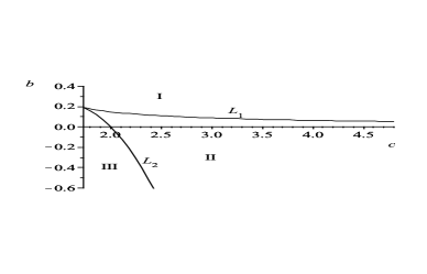
(a)

Figure 1: The bifurcation sets and bifurcation curves of system (2.7) for the parameter $c>\sqrt{3}$.

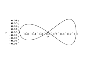
(a)

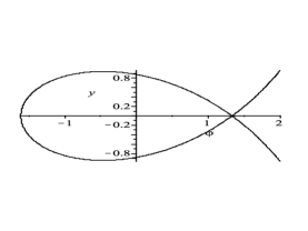
(b)

Figure 2: The phase portraits of system (2.7) when the parameters $c>\sqrt{3}$, $a=-1$ and $b=-\frac{2c^{3}}{27}+\frac{c}{3}$. (a) $c=1.8$; (b) $c=4$.

3 Solitary-wave solutions to system (1.3)

From the discussions in Section 2, we can see that, when the parameters $a=-1$, $(b,c)\in(\mathrm{II})$, system (2.7) has infinite many saddle points. So there are infinite many homoclinic orbits and system (1.3) has infinite many solitary-wave solutions accordingly.

In order to obtain exact expressions for solitary-wave solutions, we fix $b=-\frac{2c^{3}}{27}+\frac{c}{3}$.

Case I: $\sqrt{3}<c<3$

In this case, there are two homoclinic orbits connecting with the saddle point $(\frac{c}{3},0)$, see Fig. 2(a) for an example. The two homoclinic orbits of system (2.7) or (2.5) can be expressed respectively as

$$y=\pm\frac{(\varphi-\frac{c}{3})\sqrt{-\varphi^{2}+\frac{2c}{3}\varphi+\frac{5c^{2}}{9}-2}}{\varphi-c}\quad\textrm{for}\quad\varphi_{-}\leq\varphi\leq\frac{c}{3},$$ (3.1)

$$y=\pm\frac{(\varphi-\frac{c}{3})\sqrt{-\varphi^{2}+\frac{2c}{3}\varphi+\frac{5c^{2}}{9}-2}}{\varphi-c}\quad\textrm{for}\quad\frac{c}{3}\leq\varphi\leq\varphi_{+},$$ (3.2)

where $\varphi_{\pm}=\frac{1}{3}(c\pm\sqrt{6c^{2}-18})$.

Substituting (3.1), (3.2) into the first equation of system (2.5), respectively, and integrating along the corresponding homoclinic orbit, we have

$$\int_{\varphi_{-}}^{\varphi}{\frac{s-c}{(s-\frac{c}{3})\sqrt{-s^{2}+\frac{2c}{3}s+\frac{5c^{2}}{9}-2}}}ds=\frac{\sqrt{2}}{2}|\xi|,$$ (3.3)

$$\int_{\varphi}^{\varphi_{+}}{\frac{s-c}{(s-\frac{c}{3})\sqrt{-s^{2}+\frac{2c}{3}s+\frac{5c^{2}}{9}-2}}}ds=-\frac{\sqrt{2}}{2}|\xi|,$$ (3.4)

It follows from (3.3), (3.4) that

$$\frac{\pi}{2}+\arctan(\alpha(\varphi))+\frac{2c}{\sqrt{6c^{2}-18}}\ln(\beta(\varphi))=\frac{\sqrt{2}}{2}|\xi|,\quad\varphi_{-}\leq\varphi\leq\frac{c}{3},$$ (3.5)

and

$$\frac{\pi}{2}-\arctan(\alpha(\varphi))-\frac{2c}{\sqrt{6c^{2}-18}}\ln(-\beta(\varphi))=\frac{\sqrt{2}}{2}|\xi|,\quad\frac{c}{3}\leq\varphi\leq\varphi_{+},$$ (3.6)

where

$$\alpha(\varphi)=\frac{3\varphi-c}{\sqrt{-9\varphi^{2}+6c\varphi+5c^{2}-18}}$$

,

$$\beta(\varphi)=\frac{\sqrt{6c^{2}-18}+\sqrt{-9\varphi^{2}+6c\varphi+5c^{2}-18}}{c-3\varphi}.$$ (3.7)

Therefore, we obtain two solitary-wave solutions to system (1.3) in the following parametric forms:

$$\left\{{\begin{array}[]{l}\xi=\pm\sqrt{2}(\frac{\pi}{2}+\arctan(\alpha(\varphi))+\frac{2c}{\sqrt{6c^{2}-18}}\ln(\beta(\varphi)),\\ \varphi=\varphi,\\ \end{array}}\right.\;\quad(\varphi_{-}\leq\varphi\leq\frac{c}{3}),$$ (3.8)

$$\left\{{\begin{array}[]{l}\xi=\pm\sqrt{2}(\frac{\pi}{2}+\arctan(\alpha(\varphi))+\frac{2c}{\sqrt{6c^{2}-18}}\ln(\beta(\varphi)),\\ \psi=\frac{g_{2}}{\varphi-c},\\ \end{array}}\right.\;\quad(\varphi_{-}\leq\varphi\leq\frac{c}{3}),$$ (3.9)

and

$$\left\{{\begin{array}[]{l}\xi=\pm\sqrt{2}(\frac{\pi}{2}-\arctan(\alpha(\varphi))-\frac{2c}{\sqrt{6c^{2}-18}}\ln(-\beta(\varphi)),\\ \varphi=\varphi,\\ \end{array}}\right.\;(\frac{c}{3}\leq\varphi\leq\varphi_{+}),$$ (3.10)

$$\left\{{\begin{array}[]{l}\xi=\pm\sqrt{2}(\frac{\pi}{2}-\arctan(\alpha(\varphi))-\frac{2c}{\sqrt{6c^{2}-18}}\ln(-\beta(\varphi)),\\ \psi=\frac{g_{2}}{\varphi-c},\\ \end{array}}\right.\;(\frac{c}{3}\leq\varphi\leq\varphi_{+}).$$ (3.11)

Now we take a set of data and employ Maple to display the graphs of the above obtained solitary-wave solutions in Fig. 3.

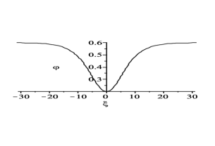
(a)

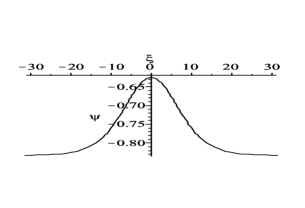
(b)

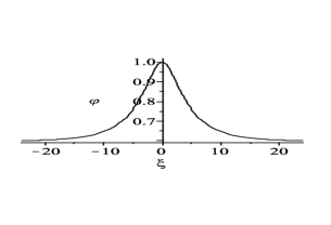
(c)

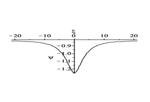
(d)

Figure 3: Solitary-wave solutions to system (1.3) when the parameters $c=1.8$, $a=-1$, $b=0.168000$ and $g_{2}=1$.

Case II: $c\geq 3$ In this case, there is one homoclinic orbit connecting with the saddle point $(\frac{c}{3},0)$, see Fig. 2(b) for an example. Similar to the Case I, we can obtain a solitary-wave solution to system (1.3), given as (3.8), (3.9). A typical such solution is shown in Fig. 4.

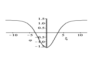
(a)

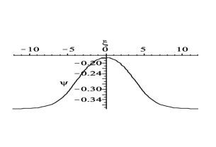
(b)

Figure 4: Solitary-wave solution to system (1.3) when the parameters $c=4$, $a=-1$, $b=-3.407407$ and $g_{2}=1$.

4 Conclusion

In summary, by using the bifurcation method, we obtain analytic expressions for smooth solitary-wave solutions to a dual equation of the Kaup-Boussinesq system (1.3). The results of this paper suggest that, in addition to solving many single-component partial differential equations, the bifurcation method can be used to obtain travelling-wave solutions of two-component systems.

References

- [1] R. Camassa, D. D. Holm, An integrable shallow water equation with peaked solitons, Phys. Rev. Lett. 71 (1993) 1661-1664.
- [2] A. Constantin, W. Strauss, Stability of the Camassa-Holm solitons, J. Nonlinear Sci. 12 (2002) 415-422.
- [3] R. S. Johnson, On solutions of the Camassa-Holm equation, Proc. Roy. Soc. London A 459 (2003) 1687-1708.
- [4] A. Parker, Wave dynamics for peaked solitons of the Camassa-Holm equation, Chaos Solitons Fractals 35 (2008) 220-37.
- [5] A. Parker, Cusped solitons of the Camassa-Holm equation. II. Binary cusponsoliton interactions, Chaos Solitons Fractals 41 (2009) 1531-1549.
- [6] V. O. Vakhnenko, E. J. Parkes, Periodic and solitary-wave solutions of the Degasperis-Procesi equation, Chaos Solitons Fractals 20 (2004) 1059-1073.
- [7] J. Lenells, Traveling wave solutions of the Degasperis-Procesi equation, J. Math. Anal. Appl. 306 (2005) 72-82.
- [8] J. H. He, X. H. Wu, Construction of solitary solution and compacton-like solution by variational iteration method, Chaos Solitons Fractals 29 (2006) 108-113.
- [9] A. Parker, Cusped solitons of the Camassa-Holm equation. I. Cuspon solitary wave and antipeakon limit, Chaos Solitons Fractals 34 (2007) 730-739.
- [10] E. J. Parkes, Some periodic and solitary travelling-wave solutions of the short-pulse equation, Chaos Solitons Fractals 36 (2008) 154-159.
- [11] I. Mustafa, New solitary wave solutions with compact support and Jacobi elliptic function solutions for the nonlinearly dispersive Boussinesq equations, Chaos Solitons Fractals 37 (2008) 792-798.
- [12] F. Khanib, S. Hamedi-Nezhadc, M. T. Darvishia, Sang-Wan Ryua, New solitary wave and periodic solutions of the foam drainage equation using the Exp-function method, Nonlinear Anal. RWA 10 (2009) 1904-1911.
- [13] S. Abbasbandy, Solitary wave solutions to the modified form of Camassa-Holm equation by means of the homotopy analysis method, Chaos Solitons Fractals 39 (2009) 428-435.
- [14] P. Guha, Geodesic flow on extended bott-virasoro group and generalized two-component peakon type dual systems, Rev. Math. Phys. 20 (2008) 1191-1208.
- [15] D. J. Kaup, Finding eigenvalue problems for solving nonlinear evolution equations, Progr. Theoret. Phys. 54 (1975) 72-78.
- [16] A. O. Smirnov, Real finite gap regular solutions of the Kaup-Boussinesq equation, Theoret. Math. Phys. 66 (1986) 19-31.
- [17] A. B. Borisov, M. P. Pavlov, S. A. Zykov, Proliferation scheme for Kaup-Boussinesq system, Physica D (152/153) (2001) 104-109.
- [18] A. M. Kamchatnov, R. A. Kraenkel, B. A. Umarov, Asymptotic soliton train solutions of Kaup-Boussinesq equations, Wave Motion 38 (2003) 355-365.
- [19] G. A. El, R. H. J. Grimshaw, M. V. Pavlov, Integrable shallow-water equations and undular bores, Stud. Appl. Math. 106 (2001) 157-186.
- [20] V. B. Matveev, M. I. Yavor, Almost periodical solutions of nonlinear hydrodynamic equation of Kaup, Ann. Inst. H. Poincar , Sect. A 31 (1979) 25-41.
- [21] E. Yomba, The extended Fan’s sub-equation method and its application to KdV-MKdV, BKK and variant Boussinesq equations, Phys. Lett. A 336 (2005) 463-476.
- [22] J. B. Li, Z. R. Liu, Travelling wave solutions for a class of nonlinear dispersive equations, Chin. Ann. Math. Ser. B 23 (2002) 397-418
- [23] M. L. Wang, Solitary wave solutions of variant Boussinesq equations, Phys. Lett. A 199 (1995) 169-172
- [24] Z. Y. Yan, H. Q. Zhang, New explicit and exact travelling wave solutions for a system of variant Boussinesq equations in mathematical physics, Phys. Lett. A 252 (1999) 291-296.
- [25] D. Z. Lü, Jacobi elliptic function solutions for two variant Boussinesq equations, Chaos Solitons Fractals 24 (2005) 1373-1385.
- [26] J. F. Zhang, Multi-solitary wave solutions for variant Boussinesq equations and Kupershmidt equations, Appl. Math. Mech. 21 (2000) 193-198
- [27] Y. B. Yuan, D. M. Pu, S. M. Li, Bifurcations of travelling wave solutions in variant Boussinesq equations, Appl. Math. Mech. 27 (2006) 811-822.
- [28] E. G. Fan, Two new applications of the homogeneous balance method, Phys. Lett. A 265 (1998) 353-357.
- [29] E. Fan, Y. Hon, A series of traveling wave solutions for two variant Boussinesq equations in shallow water waves, Chaos Solitons Fractals 15 (2003) 559-566.
- [30] D. Luo, et al., Bifurcation Theory and Methods of Dynamical Systems, World Scientific Publishing Co., London, 1997.
- [31] S. N. Chow, J. K. Hale, Method of Bifurcation Theory, Springer, New York, 1981.
- [32] J. Guckenheimer, P. Holmes, Nonlinear Oscillations, Dynamical Systems and Bifurcation of Vector Fields, Springer, New York, 1983.
- [33] L. Perko, Differential Equations and Dynamical Systems, Springer, New York, 1991.
- [34] J. B. Li, Z. R. Liu, Smooth and non-smooth traveling waves in a nonlinearly dispersive equation, Appl. Math. Model. 25 (2000) 41-56.
- [35] T. F. Qian, M. Y. Tang, Peakons and periodic cusp wave in a generalized Camassa-Holm equation, Chaos Solitons Fractals 12 (2001) 1347-1360.
- [36] J. W. Shen, W. Xu, Bifurcations of smooth and non-smooth traveling wave solutions in the generalized Camassa-Holm equation, Chaos Solitons Fractals 26 (2005) 1149-1162.
- [37] L. J. Zhang, L. Q. Chen, X. W. Huo, Peakons and periodic cusp wave solutions in a generalized Camassa-Holm equation, Chaos Solitons Fractals 30 (2006) 1238-1249.
- [38] Z. R. Liu, Z. R. Ouyang, A note on solitary waves for modified forms of Camassa-Holm and Degasperis-Procesi equations, Phys. Lett. A 366 (2007) 377-381.
- [39] J. B. Zhou, L. X. Tian, Soliton solution of the osmosis equation, Phys. Lett. A 372 (2008) 6232-6234.
- [40] A. Y. Chen, W. T. Huang, S. Q. Tang, Bifurcations of travelling wave solutions for the Gilson-Pickering equation, Nonlinear Anal. RWA 10 (2009) 2659-2665.
- [41] J. B. Zhou, L. X. Tian, Solitons, peakons and periodic cusp wave solutions for the Fornberg-Whitham equation, Nonlinear Anal. RWA (2009), in press (doi:10.1016/j.nonrwa.2008.11.014).
- [42] J. B. Zhou, L. X. Tian, X. H. Fan, Soliton, kink and antikink solutions of a 2-component of the Degasperis-Procesi equation, Nonlinear Anal. RWA (2009), in press (doi:10.1016/j.nonrwa.2009.08.009).