Generation of equatorial jets by large-scale latent heating on the giant planets

Abstract

Three-dimensional numerical simulations show that large-scale latent heating resulting from condensation of water vapor can produce multiple zonal jets similar to those on the gas giants (Jupiter and Saturn) and ice giants (Uranus and Neptune). For plausible water abundances (3–5 times solar on Jupiter/Saturn and 30 times solar on Uranus/Neptune), our simulations produce $\sim 20$ zonal jets for Jupiter and Saturn and 3 zonal jets on Uranus and Neptune, similar to the number of jets observed on these planets. Moreover, these Jupiter/Saturn cases produce equatorial superrotation whereas the Uranus/Neptune cases produce equatorial subrotation, consistent with the observed equatorial jet direction on these planets. Sensitivity tests show that water abundance, planetary rotation rate, and planetary radius are all controlling factors, with water playing the most important role; modest water abundances, large planetary radii, and fast rotation rates favor equatorial superrotation, whereas large water abundances favor equatorial subrotation regardless of the planetary radius and rotation rate. Given the larger radii, faster rotation rates, and probable lower water abundances of Jupiter and Saturn relative to Uranus and Neptune, our simulations therefore provide a possible mechanism for the existence of equatorial superrotation on Jupiter and Saturn and the lack of superrotation on Uranus and Neptune. Nevertheless, Saturn poses a possible difficulty, as our simulations were unable to explain the unusually high speed ($\sim 400\rm\,m\,s^{-1}$) of that planet’s superrotating jet. The zonal jets in our simulations exhibit modest violations of the barotropic and Charney-Stern stability criteria. Overall, our simulations, while idealized, support the idea that latent heating plays an important role in generating the jets on the giant planets.

1 Introduction

The question of what causes the prominent east-west (zonal) jet streams and banded cloud patterns on Jupiter, Saturn, Uranus, and Neptune remains a major unsolved problem in planetary science. On Jupiter and Saturn, there exist $\sim 20$–30 jets, including a broad, fast superrotating (eastward) equatorial jet. In contrast, Uranus and Neptune exhibit only $\sim 3$ jets each, with high-latitude eastward jets and a subrotating (westward) equatorial jet. All four planets also exhibit a variety of compact vortices, waves, turbulent filamentary regions, short-lived convective events, and other local features. Recent observational studies demonstrate that small eddies pump momentum up-gradient into the zonal jets on Jupiter and Saturn (Salyk et al., 2006; Del Genio et al., 2007), which strongly suggests that cloud-layer processes are important in jet formation, although this does not exclude a possible role for the deep interior too. Scenarios to explain these diverse observations range from the “shallow-forcing” scenario, in which jet generation occurs via injection of turbulence, absorption of solar radiation and latent heat release in the cloud layer, to the “deep-forcing” scenario, in which the jet formation results from convection occurring throughout the molecular envelope (for reviews see Ingersoll et al., 2004; Vasavada and Showman, 2005). Over the past several decades, a variety of idealized models have been developed that successfully produce banded zonal flows reminiscent of those on the giant planets (Williams, 1978; Cho and Polvani, 1996a; Huang and Robinson, 1998; Heimpel and Aurnou, 2007; Lian and Showman, 2008).

Despite these successes, the equatorial jet direction and magnitude have proved to be formidable puzzles that are difficult to explain. Many published models predict the same equatorial jet direction for all four giant planets and thereby fail to provide a coherent explanation that encompasses both the gas giants (Jupiter/Saturn) and the ice giants (Uranus/Neptune). Under relevant conditions, one-layer shallow-water-type models generally produce westward equatorial flow for all four planets (Cho and Polvani, 1996b; Iacono et al., 1999; Showman, 2007; Scott and Polvani, 2007), consistent with Uranus and Neptune but not Jupiter and Saturn. In the parameter regime of giant planets, some shallow-water models have produced equatorial superrotation (Scott and Polvani, 2008), but as yet these models make no predictions for why superrotation should occur on Jupiter and Saturn but not Uranus and Neptune. Some recent three-dimensional (3D) shallow-atmosphere models can also produce equatorial superrotation under specific conditions (Williams, 2006, 2002, 2003a, 2003b, 2003c; Yamazaki et al., 2005; Lian and Showman, 2008), but this has generally required the addition of ad hoc forcing, and even if such forcing were plausible, it is unclear why it would occur on Jupiter/Saturn but not Uranus/Neptune. In contrast, the deep convection models produce equatorial superrotation in most cases (Aurnou and Olson, 2001; Christensen, 2001; Heimpel et al., 2005; Heimpel and Aurnou, 2007; Glatzmaier et al., 2008), consistent with Jupiter and Saturn but inconsistent with Uranus and Neptune. In the context of deep convection models, Aurnou et al. (2007) proposed that Uranus and Neptune are in a regime where geostrophy breaks down in the interior, leading to turbulent mixing of angular momentum and a westward equatorial jet. However, this mechanism occurs only at heat fluxes greatly exceeding than those observed on Uranus and Neptune (Aurnou et al., 2007). Moreover, given that the heat fluxes on Jupiter and Saturn exceed those on Uranus and Neptune, one might expect the mechanism to apply more readily to the former pair than the latter pair; if so, one should see equatorial subrotation on Jupiter/Saturn yet superrotation on Uranus/Neptune, backward from the observed equatorial jet directions. Schneider and Liu (2009) developed a 3D numerical model that produced banded zonal jets and an equatorial superrotation on Jupiter. This is the first model that combines the deep convection (via a simple convective adjustment scheme) and absorption of solar radiation in a shallow atmosphere. However, their model extends to only 3 bars pressure and thus neglects the effects of latent heating, which may be crucial in generating horizontal temperature contrasts in the cloud layer. Furthermore, it is unclear whether their model can produce equatorial subrotation on Uranus and Neptune by the same mechanism. It is fair to say that we presently lack a coherent explanation for the equatorial jets that encompasses both the gas giants (Jupiter/Saturn) and the ice giants (Uranus/Neptune).

Here, we test the hypothesis that large-scale latent heating associated with condensation of water vapor can pump the zonal jets on the four giant planets. This hypothesis has been repeatedly suggested over the past 40 years (Barcilon and Gierasch, 1970; Gierasch, 1976; Ingersoll et al., 2000; Gierasch et al., 2000), but this idea has not yet been adequately tested in numerical models. While observations cannot yet constrain the existence of large-scale latent heating, abundant evidence nevertheless exists for moist convection on the giant planets. Lightning has been identified in nightside images of Jupiter from Voyager, Galileo, Cassini, and New Horizons; these flashes typically occur within localized, opaque clouds that grow to diameters up to $\sim 3000\,$km over a few days, indicating convective activity. The lightning illuminates finite regions on the cloud deck, indicating that the flashes occur at depths of 5–10 bars, in the expected water condensation region (Borucki and Williams, 1986; Dyudina et al., 2002). Near such storms, clouds are sometimes observed whose tops are deeper than 4 bars, where the only condensate is water (Banfield et al., 1998; Gierasch et al., 2000). On Saturn, electrostatic discharges presumably caused by lightning have been identified, as have explosive convective clouds that probably cause them (Porco et al., 2005; Dyudina et al., 2007). Whistlers and electrostatic discharges indicating the presence of lightning have also been detected on Uranus and Neptune (Zarka and Pedersen, 1986; Gurnett et al., 1990; Kaiser et al., 1991), suggesting that moist convection occurs on these planets too. For plausible water abundances (a few times solar or greater), latent heating can cause local temperature increases great enough to have important meteorological effects.

To date, numerical models of jet formation have generally not included moisture and its latent heat release. Most two-dimensional (2D) and shallow-water models adopt forcing that injects turbulence everywhere simultaneously and is confined to a small range of wavenumbers (e.g. Huang and Robinson, 1998; Scott and Polvani, 2007), which does not capture the sporadic and localized nature of moist-convective events. Likewise, existing 3D models of Jovian jet formation have been dry (no water vapor) and force the flow by imposing latitudinal temperature differences rather than including moist convection (e.g. Williams, 2006, 2002, 2003a, 2003b, 2003c; Yamazaki et al., 2005; Lian and Showman, 2008). Notable efforts in the right direction are the one-layer studies by Li et al. (2006) and Showman (2007), which adopted a forcing explicitly intended to represent the effects of moist convection. Li et al. (2006) adopted a quasigeostrophic model and introduced isolated vorticity patches to represent moist-convective storms; Showman (2007) adopted the shallow-water equations and introduced isolated mass pulses to represent the moist convection. These studies show that, under planetary rotation, the small-scale turbulent flow can inverse cascade to form large scale dynamics: zonal jets dominate at low latitudes and vortices dominate at high latitudes. Nevertheless, these models do not explicitly include water vapor, and the moist convection events are, rather than occurring naturally, injected by hand with prescribed sizes, lifetimes and amplitudes. Studies have also been carried out that investigate the effects of sophisticated cloud microphysics schemes on the vertical structure in 1D column models (Del Genio and McGrattan, 1990) and 2D height/latitude models (Nakajima et al., 2000; Palotai and Dowling, 2008), but these studies do not address whether moist convection can pump the jets.

Our previous 3-D studies with imposed latitudinal temperature variation can produce baroclinic eddies that drive the zonal jets through inverse-cascade of turbulence (Lian and Showman, 2008). Those simulations successfully reproduced some major dynamic features on Jupiter such as banded zonal winds and equatorial superrotation; they also predicted that the jets on Jupiter could extend significantly deeper than the eddy accelerations that pump them. However, the nature of the imposed forcing schemes was only a crude parameterization of the processes that produce latitudinal temperature contrasts.

Here we present three-dimensional (3D) global numerical simulations using the MITgcm to investigate whether large-scale latent heating can drive the zonal jets on Jupiter, Saturn, Uranus, and Neptune. Specifically, we investigate whether we can explain (i) the approximate number and speed of jets, and (ii) the direction of the equatorial jet on all four planets in the context of a single mechanism. We explicitly include water vapor as a tracer in our numerical model. Section 2 describes the numerical model, section 3 presents the simulation results, and section 4 concludes.

2 Models

2.1 Model setup

We use a global circulation model, the MITgcm, to solve the 3D hydrostatic primitive equations in pressure coordinates on a sphere. Previous studies of jet formation on the giant planets have adopted dry models (Lian and Showman, 2008; Williams, 2003c; Showman, 2007; Scott and Polvani, 2007; Li et al., 2006), but here we explicitly treat the transport and condensation of water vapor. Condensation occurs whenever the relative humidity exceeds 100%, and the resultant latent heating is explicitly added to the energy equation.

The system is governed by the horizontal momentum, hydrostatic equilibrium, mass continuity, energy, and water-vapor equations as follows:

$${{d{\bf v}}\over{dt}}+f\hat{k}\times{\bf v}+\nabla_{p}\Phi=0$$ (1)

$${\partial{{\Phi}}\over{\partial{p}}}=-{1\over\rho}$$ (2)

$$\nabla_{p}\cdot{\bf v}+{\partial{\omega}\over{\partial{p}}}=0$$ (3)

$${d\theta\over{dt}}=Q_{\theta}+{L\over c_{p}}{\theta\over T}(\delta{{q-q_{s}}\over{\tau_{s}}})$$ (4)

$${dq\over{dt}}=-{{q-q_{s}}\over\tau_{s}}\delta+Q_{\rm deep}$$ (5)

where ${\bf v}$ is the horizontal wind vector (comprised of zonal wind $u$ and meridional wind $v$), $\omega=dp/dt$ is vertical wind in pressure coordinates, $f=2\Omega\sin\phi$ is the Coriolis parameter (where $\phi$ is latitude and $\Omega$ is the rotation rate of the planet), $\Phi$ is geopotential, $\hat{k}$ is the unit vector in the vertical direction (positive upward), $\rho$ is density, $\nabla_{p}$ is the horizontal gradient operator at a given pressure level, $d/dt$ is the total derivative operator given by $d/dt=\partial/\partial t+{\bf v}\cdot\nabla_{p}+\omega\partial/\partial p$, $q$ is the water-vapor mixing ratio (defined as kilograms of water vapor per kilogram of dry H₂ air), and $\theta=T(p_{0}/p)^{\kappa}$ is potential temperature. Here $T$ is temperature and $\kappa\equiv R/c_{p}$, which is a specified constant, is the ratio of the gas constant to the specific heat at constant pressure. In the equations above, density $\rho$ is calculated at a given temperature and pressure from the ideal gas law, $\rho=\frac{pm}{R_{u}T}$, where $R_{u}$ is the universal gas constant and $m$ is the mean molecular mass of the moist air, given by $m=\frac{m_{H_{2}}}{1+q/\epsilon}+q\frac{m_{H_{2}}}{1+q/\epsilon}$, where $\epsilon=\frac{m_{H_{2}O}}{m_{H_{2}}}$ is the ratio of the mass of a water molecule to the mass of dry air molecule. Note that we neglect the density perturbation associated with condensate mass loading. Given the density field, geopotential $\Phi$ is then calculated by integrating the hydrostatic equation vertically via Eq. (2). The reference pressure $p_{0}$ is taken as $1\,$bar (note, however, that the dynamics are independent of the choice of $p_{0}$). Curvature terms are included in ${\bf v}\cdot\nabla{\bf v}$. In all governing equations Eq. 1 – Eq. 5, the dependent variables ${\bf v}$, $\omega$, $\Phi$, $\rho$, $\theta$, and $q$ are functions of longitude $\lambda$, latitude $\phi$, pressure $p$, and time $t$.

The water-vapor equation (Eq. 5) governs the time evolution of the water-vapor mixing ratio $q$. There are two source/sink terms. The first, $-(q-q_{s})\delta/\tau_{s}$, represents loss through condensation. We apply an “on-off switch” $\delta$ to make the condensation events occur only when the environment is supersaturated: when $q>q_{s}$ then $\delta=1$ and water vapor condenses; when $q\leq q_{s}$ then $\delta=0$ and water vapor does not condense. Here $q_{s}$ is the saturated water-vapor mixing ratio, given by the approximate expression

$$q_{s}={m_{H_{2}O}\over{m_{H_{2}}}}{{e_{s}}\over p},$$ (6)

$$e_{s}={e_{0}}exp{[-{L\over{R_{v}}}({1\over T}-{1\over{T_{0}}})]},$$ (7)

where $e_{s}$ is the saturation vapor pressure. Other constants in Eqs. 6–7 are given as follows: $e_{0}=609.14\,\,{\rm Pa}$ is a reference saturation water-vapor pressure at temperature $T_{0}=273\,{\rm K}$, $R_{v}=461.0\rm JK^{-1}kg^{-1}$ is the specific gas constant of water vapor, $m_{H_{2}O}$ is the molecular mass of water and $m_{H_{2}}$ is the molecular mass of hydrogen gas. The quantity $\tau_{s}$ is the condensation timescale, generally taken as $10^{4}\,$sec (almost 3 hours), representative of a typical convective time. The second term, $Q_{\rm deep}$, represents a source of water vapor applied near the bottom of the model (see below).

When condensation occurs, we apply the appropriate latent heating to the energy equation (second term on right side of Eq. 4). The specific latent heat of condensation is given by $L=2.5\times 10^{6}\rm\,J\,kg^{-1}$.

Palotai and Dowling (2008) point out, using simplified one- and two-dimensional test cases, that cloud microphysics can interact with large-scale dynamics on giant planets. While recognizing that inclusion of microphysics in 3D is an important goal for future work, we here make the simplifying assumption that all of the condensate instantaneously rains out the bottom of the model. This allows us neglect cloud microphysics and thereby sidestep the numerous complications associated with cloud-particle growth and settling, the evaporation of falling precipitation, and other microphysical processes that remain poorly understood — and whose effects must be parameterized in large-scale models. Depending on the complexity of the adopted schemes, including such processes can introduce potentially dozens of new free parameters into the model. In Earth climate models, these parameters are generally tuned using a combination of laboratory and field data, but it is unclear to what extent such parameter values (or even the schemes themselves) translate into the giant planet context (for discussion see Palotai and Dowling, 2008). Given these difficulties, there is strong merit in exploring the dynamics in the limiting case without microphysics, as presented here.

True moist convection, which involves the formation of cumulus clouds and thunderstorms, occurs on length scales much smaller than the horizontal grid resolutions achievable in most global-scale models (including ours). Significant work has gone into developing sub-grid-scale cumulus parameterization schemes to represent the effects of this cumulus convection on the large-scale flow resolved by global models (for reviews see, e.g., Emanuel and Raymond, 1993; Arakawa, 2004). Incorporating such a scheme into a Jovian model is a worthy goal, but such schemes are often complex, and it is first useful to ascertain the effects of large-scale latent heating, that is, latent heating associated with the hydrostatically balanced circulation explicitly resolved by the model. This is the approach we pursue here.

In general, we expect that the latent heating and decrease in molecular mass accompanying condensation/rainout will lead to a vertical structure where potential temperature increases with height and molecular mass decreases with height. If so, this would imply that condensation would stabilize the environment against convection, leading to a virtual potential temperature that increases with height. Given this expectation, we do not include any dry convective adjustment scheme in the current simulations.

To provide a crude representation of evaporating precipitation and water vapor mixed upward from the deeper atmosphere (below the bottom of our domain), we apply a source term of water vapor, $Q_{\rm deep}$, to the bottom of the model. This term takes the form $Q_{\rm deep}=(q_{\rm deep}-q)/\tau_{\rm replenish}$ and is applied only at pressures exceeding a critical pressure $p_{c}$, which is chosen to be deeper than the deepest possible condensation pressure for the water-vapor abundance and thermal structure expected in a given simulation. Here, $q_{\rm deep}$ is a specified planetary water vapor abundance (e.g., 1, 3, 10, or 30 times solar) and $\tau_{\rm replenish}$ is a relaxation time. Our goal is to force the deep water abundance (at $p>p_{c}$) to be very close to $q_{\rm deep}$. The relaxation time, $\tau_{\rm replenish}$, is thus not a free parameter and is chosen to be very short (typically 5 hours). This source term allows the model to reach a statistical steady state in which the mean total water vapor content of the atmosphere is nearly constant over time — despite the loss of water via condensation.

In the thermodynamic equation (Eq. 4), $Q_{\theta}$ is the rate of heating (expressed in ${\rm K}\,{\rm sec}^{-1}$) due to radiation. We adopt a simple Newtonian relaxation scheme:

$$Q_{\theta}=-{{\theta-\theta_{\rm ref}}\over{\tau_{\rm rad}}}$$ (8)

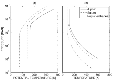
Figure 1: Reference temperature-pressure profile for giant planets.

The equilibrium $\theta_{\rm ref}$ profiles, shown in Fig. 1, are based on pressure-temperature profiles following the radio-occultation and Galileo-probe results (Lindal et al., 1981, 1985, 1987; Lindal, 1992; Seiff et al., 1998). Each contains a deep neutrally stable troposphere, an isothermal stratosphere and a smooth transition layer between the two regions (Fig. 1). The adopted relaxation timescales are 400 Earth days for Jupiter-type simulations and 200 Earth days for Neptune-type simulations. These timescales are shorter than expected radiative timescales in the deep tropospheres of giant planets but allow us to perform simulations in reasonable time while preserving the quasi-isentropic behavior of the atmospheric motions over typical dynamical timescales of 1–10 days.

Importantly, we chose to make $\theta_{\rm ref}$ independent of latitude for this study. This contrasts with previous studies (e.g., Lian and Showman, 2008; Williams, 2002, 2003b), where the equilibrium temperature $\theta_{\rm ref}$ is a function of latitude. Our choice here is motivated by the fact that when $\theta_{\rm ref}$ depends on latitude, the forcing imposes a zonally banded structure on the flow, and it is thus unclear to what extent any zonal jet formation result from such banded forcing rather than from the $\beta$ effect (where $\beta$ is the gradient of Coriolis parameter with northward distance). By making $\theta_{\rm ref}$ independent of latitude, we can ensure that any banded flow structures result from $\beta$, not from anisotropic forcing. Moreover, when $\theta_{\rm ref}$ depends on latitude, then not only the latent heating but the radiation cause latitudinal temperature differences and thus injects available potential energy (APE) into the flow. The energy source driving the flow would thus be ambiguous. Here, we specifically aim to test whether large-scale latent heating can drive Jovian-type jets, and by maintaining $\theta_{\rm ref}$ constant with latitude, we ensure that the only mechanism for generating lateral temperature contrasts (hence APE) is large-scale latent heating.

The upper boundary in our simulations is zero pressure and impermeable. The lower boundary corresponds to an impermeable wall at a constant height; because the pressure can vary along this surface, it is implemented in pressure coordinates as a free surface through which no mass flow can occur (see Campin et al. (2004) for details). Both boundaries are free-slip in horizontal velocity The mean bottom pressure of simulated domain is a free parameter which varies from 100 to 500 bars depending on the simulation. We adopt the ideal gas equation of state. The simulations include no explicit viscosity, but a fourth-order Shapiro filter (Shapiro, 1970) (analogous to eighth-order hyperviscosity) is added to maintain numerical stability. The time step is 100 sec.

Initially there are no winds in our simulations. The abundance of water vapor is set to be subsaturated ($\rm 95\%$ of saturation) in the region where $p<p_{c}$ and $q_{\rm deep}$ at $p>p_{c}$. In the initial condition, we introduce 5–9 random temperature perturbations at pressures less than $p_{c}$ to break the horizontal symmetry and initiate motions. Each of the initial perturbations, which are positioned randomly within the simulated domain, has a warm center and affects the temperature radially within $\rm 5^{\circ}$. The initial perturbations for our Jupiter, Saturn, and Uranus/Neptune cases adopt $\Delta{\theta}=5$, 5, and 10 K, respectively, and are confined to pressures less than 7, 10, and 10 bars, respectively. We performed tests that varied the initial location and number of these perturbations, which show that the qualitative final dynamical state, including the equatorial jet direction, is not sensitive to the number of perturbations or their locations. The main purpose of the perturbations is to induce sufficient motion to generate supersaturation in localized regions only at the very beginning of the simulations; once this occurs, the circulation becomes self-generating.

Although the water abundances on Jupiter, Saturn, Uranus, and Neptune are unknown, Galileo probe data indicate that Jupiter’s C, N, S, Ar, Kr, and Xe abundances are all between 2–4 times solar. Spectroscopic information suggests that methane is 7 times solar on Saturn (Flasar et al., 2005) and 30–40 times solar on Uranus and Neptune (Fegley et al., 1991; Baines et al., 1995). These values suggest that the water abundance is modest at Jupiter, intermediate at Saturn, and large at Uranus and Neptune. Predicted condensation pressures are $\sim 8\,$bars for Jupiter, $\sim 20\,$bars for Saturn, and 200–300 bars on Uranus and Neptune, depending on the water abundance (Flasar et al., 2005; Fegley et al., 1991; Baines et al., 1995).

We explore a range of deep water-vapor abundances from 1–20 times solar on Jupiter and Saturn and from 1–30 times solar on Uranus and Neptune. Combined with the prescribed temperature structure (see Fig. 1), these abundances determine the range of pressures over which condensation will occur in any given simulation. We then set $p_{c}$, the pressure at the top of our deep water vapor source $Q_{\rm deep}$, to be deeper than the base of the condensation region. We use $p_{c}=7\,\rm bars$ with 3 times solar water abundance and $p_{c}=10\,\rm bars$ with 10 times solar water abundance for Jupiter simulations. For Saturn, we used $p_{c}=17.3\,$bars for 5 times solar and $19.2\,$bars for 10 times solar water abundance. On Neptune, we use $p_{c}=120\,\rm bars$ with 1 times solar water abundance, $p_{c}=220\,\rm bars$ with 10 times solar water abundance and $p_{c}=330\,\rm bars$ with 30 times solar water abundance. Here 1 times solar water abundance is 0.01 kilogram of water vapor per kilogram of dry air. Among all these simulations, Jupiter-type simulation with 3 times solar water abundance and Neptune-type simulation with 30 times solar water abundance are the nominal cases.

We run simulations using the cube-sphere grid. Planetary parameters are chosen based on Jupiter, Saturn, and Neptune, the latter of which represents the Uranus/Neptune pair. The parameters we implement for the nominal simulations are listed in Table 1, where C128 stands for $\rm 128\times 128$ on each cubed-sphere face and C128 is equivalent to $\rm 512\times 256$ in longitude-latitude grid; C64 stands for $\rm 64\times 64$ on each cubed-sphere face and C64 is equivalent to $\rm 256\times 128$ in longitude-latitude grid; $N_{L}$ is number of layers in vertical direction.

Planet	$a\rm{(km)}$	$\Omega\rm{(s^{-1})}$	$c_{p}\rm{(JK^{-1}kg^{-1})}$	${\kappa}$	$g\rm{(ms^{-2})}$	${R_{q}}$	$Res$	${N_{L}}$	$p_{b}\rm{(bars)}$
Jupiter	71492	$\rm{1.7585\times 10^{-4}}$	13000	0.29	22.88	-0.8778	C128	35	100
Saturn	60268	$\rm{1.6570\times 10^{-4}}$	13000	0.29	8.96	-0.8778	C128	35	100
Neptune	24746	$\rm{1.0389\times 10^{-4}}$	13000	0.305	11.7	-0.8778	C64	38	500

Table 1: Note: $a$ is radius of planet, $\Omega$ is rotation rate, $c_{p}$ is heat capacity, $\kappa={R\over{c_{p}}}$, $g$ is gravity, $R_{q}={{1-\epsilon}\over\epsilon}$, where $\epsilon$ is the ratio of molecular mass between H₂O and H₂, $Res$ is the horizontal resolution, $N_{L}$ is the number of layers, and $p_{b}$ is the mean bottom pressure of the simulated domain.

2.2 Diagnostics

Before presenting our results, we describe the formalism we use to diagnose our simulations following Karoly et al. (1998). For any quantity $A$, we can define $A=[A]+A^{*}$ where $[A]$ denotes the zonal mean and $A^{*}$ denotes the deviation from the zonal mean. Likewise, we can define $A=\overline{A}+A^{\prime}$, where $\overline{A}$ denotes the time average and $A^{\prime}$ denotes the deviation from the time average. Inserting these definitions into the zonal momentum equation (Eq. 1) and averaging in longitude and time, we obtain

$${\partial[\overline{u}]\over\partial t}=-{\partial\over\partial y}([\overline{u^{\prime}v^{\prime}}]+[\overline{u}^{*}\overline{v}^{*}])-{\partial\over\partial p}([\overline{u^{\prime}\omega^{\prime}}]+[\overline{u}^{*}\overline{\omega}^{*}])$$

$$-[\overline{v}]{\partial[\overline{u}]\over\partial y}-[\overline{\omega}]{\partial[\overline{u}]\over\partial p}+f[\overline{v}]$$ (9)

In Eq. 9, $[\overline{u^{\prime}v^{\prime}}]$ and $[\overline{u^{\prime}\omega^{\prime}}]$, are the latitudinal and vertical fluxes of eastward momentum, respectively, associated with traveling eddies; $[\overline{u}^{*}\overline{v}^{*}]$ and $[\overline{u}^{*}\overline{\omega}^{*}]$, are the latitudinal and vertical fluxes of eastward momentum, respectively, associated with stationary eddies. This equation states that latitudinal convergence of horizontal eddy momentum flux, vertical convergence of vertical eddy momentum flux, horizontal and vertical advection and Coriolis acceleration drive the zonal winds.

3 Results

3.1 Basic flow regime

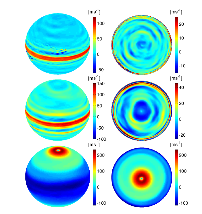
Figure 2: Snapshots of zonal winds for Jupiter simulation (top row) with 3 times the solar water abundance at 0.9-bar level, Saturn simulation (center row) with 5 times the solar water abundance at 1-bar level and Uranus/Neptune simulation (bottom row) with 30 times the solar water abundance at the 0.8-bar level. The simulation time for Jupiter and Uranus/Neptune is 1200 Earth days. The simulation time for Saturn is 1600 Earth days. The left column gives an oblique view and the right column gives a view looking down over the north pole. Our Jupiter and Saturn cases develop $\sim 20$ jets with equatorial superrotation while the Uranus/Neptune case develops 3 jets with equatorial subrotation.

Our Jupiter simulation with 3 times the solar water abundance and Uranus/Neptune simulation with 30 times the solar water abundance produce zonal winds similar to those observed on Jupiter/Saturn and Neptune/Uranus. The similarities, in general, are multiple banded zonal jets with equatorial superrotation on Jupiter/Saturn and high-latitude eastward jets with broad equatorial subrotation on Neptune/Uranus. These are shown in Fig. 2. The initial perturbations generate motion, which triggers condensation. Once the circulation is initiated, it becomes self-sustaining: horizontal temperature gradients induced by large-scale latent heating drive a circulation that continues to dredge up water vapor to the condensation region, allowing latent heating and maintaining the temperature differences. The eddies produced in this way interact with planetary rotation to generate large-scale zonal flows. The resulting zonal flow at the 1-bar level contains about 20 zonal jets for Jupiter/Saturn-type simulations and $\sim 3$ zonal jets for Uranus/Neptune-type simulations (Fig. 2).

First we examine the Jupiter simulations (Fig. 3). By 55 Earth days, the winds show significant zonality, and after $\sim 1100\,$days the jet pattern becomes relatively stable with $\sim 20$ jets. The equatorial jet builds up rapidly, reaching zonal-mean zonal wind speeds of $80\,{\rm m}\,{\rm sec}^{-1}$ and local speeds exceeding $100\,{\rm m}\,{\rm sec}^{-1}$. Initially, the jet spans only a range of longitudes (e.g., Fig. 3, second panel). Low-latitude eddies triggered by localized latent heating continuously pump energy into the equatorial flow, which eventually makes the equatorial superrotation encircle the whole globe by 116 Earth days. The longitudinal variation of this equatorial superrotation becomes small after $\sim 1000$ Earth days. The jet spans latitudes $\rm 10^{\circ}$ south to $\rm 10^{\circ}$ north with an average wind speed of $\rm 80ms^{-1}$.

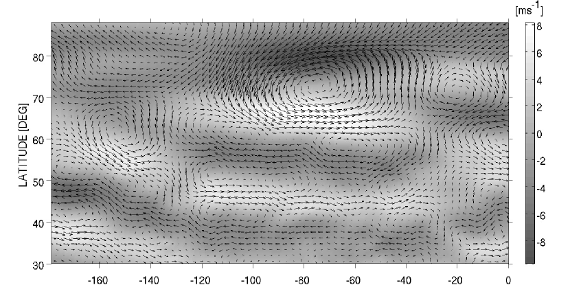
Figure 5: A zoom-in showing the wind structure in a portion of the domain for our Jupiter case with 3 times solar water. Gray scale gives zonal winds and arrows show full wind velocity at 0.9 bars. This figure is at 2315 Earth days. The wind field shown here is in longitude-latitude section from $\rm-180^{\circ}$ to $0^{\circ}$ longitude and from $\rm 30^{\circ}$ N to $90^{\circ}$N latitude.

In our Jupiter simulations, numerous alternating east-west jets also develop at higher latitudes with speeds of $\sim 5$–$10\,{\rm m}\,{\rm sec}^{-1}$. These high-latitude zonal jets extend almost to the pole (Fig. 2). Interestingly, however, the high-latitude jets are not purely zonal but develop meanders with latitudinal positions that vary in longitude, as can be seen in Figs. 2 and 5. This meandering presumably occurs because the $\beta$ effect (which is necessary for jet formation) weakens at high latitudes. As a result of these meanders, a zonal average smoothes through these jets, so the zonal-mean zonal wind profile shows minimal structure poleward of $\sim 30^{\circ}$ latitude (Fig. 3, rightmost panels); nevertheless, the high-latitude jet structure remains evident in profiles without zonal averaging (Figs. 2 and 3). I͡nterestingly, in the Saturn case, an eastward jet at $\sim 70^{\circ}$ latitude develops meanders crudely resembling a polygon when viewed from over the pole (Fig. 2). This structure may have relevance to explaining Saturn’s polar hexagon (Godfrey, 1988; Baines et al., 2009).

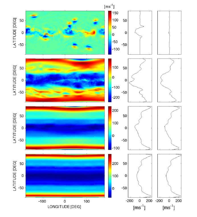
Figure 4: Snapshots of zonal winds at 0.8 bars for our Uranus/Neptune simulation with 30 times the solar water abundance. The four rows, from top down, give the state at 3, 55, 1157 and 2315 Earth days. The left column shows the zonal wind over the full globe in a rectangular projection. The middle column gives the zonal wind profile at longitude $-176.8^{\circ}$. The right column gives the zonal-mean zonal wind.

Our Uranus/Neptune simulation with 30 times the solar water abundance, however, behaves quite differently than our Jupiter and Saturn cases (Fig. 4). By $\sim 1000$ days, the profile stabilizes with three jets: a broad westward equatorial flow extending from latitudes $40^{\circ}$ south to $40^{\circ}$ north and reaching speeds of almost $-100\,{\rm m}\,{\rm sec}^{-1}$, and two high-latitude eastward jets reaching peak speeds of almost $250\,{\rm m}\,{\rm sec}^{-1}$ at latitudes of 70–$80^{\circ}$ north and south. Eddy activity, though still vigorous, is hardly visible in comparison with the zonal flow after several hundred Earth days.

As a control experiment, we also performed a Neptune simulation where latent heating and condensation were turned off (i.e., $\delta=0$ in Eqs. 4–5 regardless of the relative humidity). Because $\theta_{\rm ref}$ is independent of latitude, radiation removes rather than adds available potential energy, and thus the only source of available potential energy in this simulation is provided by the thermal perturbations in the initial condition. Consistent with this expectation, this simulation develops peak winds of only $\sim 20\rm\,m\,sec^{-1}$, an order-of-magnitude weaker than those our nominal simulation. This comparison demonstrates the crucial role that latent heating plays in generating jets in our nominal simulations.

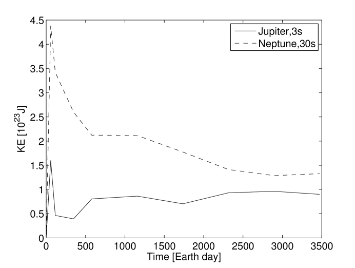
Figure 6: Total kinetic energy in region from 1 bar and above as a function of time. The solid line shows our nominal Jupiter simulation with 3 times the solar water abundance and the dashed line shows nominal Neptune simulation with 30 times the solar water abundance.

Figure. 6 shows the time evolution of kinetic energy in our Jupiter and Uranus/Neptune simulations. The kinetic energy is vertically and horizontally integrated in region from 1 bar and above. Both Jupiter and Uranus/Neptune simulations show that kinetic energy quickly spikes up in first 100 Earth days and gradually drops afterwards. After 2500 Earth days, the variation of kinetic energy becomes small, indicating the simulations get close to a steady state from top down to 1 bar. This development of kinetic energy is very similar to that of Lian and Showman (2008). Nevertheless, the barotropic winds continue to spin up at deep levels near the bottom of the model.

Our simulations provide a possible explanation for the equatorial superrotation on Jupiter/Saturn yet the equatorial subrotation on Uranus/Neptune as well as the approximate number of jets observed on all four planets. We emphasize that our simulated jet profiles — including the equatorial jet direction — are fully self-generating and emerge spontaneously, without the application of ad hoc forcing schemes. The only physical differences between the two simulations in Fig. 2 is the values of the planetary parameters (radius, rotation rate, gravity) and deep water abundance $q_{\rm deep}$; the forcing schemes are otherwise identical for the two cases. In contrast, previous shallow-atmosphere studies either produced superrotation only with artificially imposed forcing near the equator (Williams, 2003c; Yamazaki et al., 2005; Lian and Showman, 2008) or produce superrotation more naturally but make no prediction for Jupiter/Saturn versus Uranus/Neptune (Scott and Polvani, 2008; Schneider and Liu, 2009). Ours is the first study to naturally produce superrotation in a Jupiter regime yet subrotation in a Uranus/Neptune regime within the context of a single model.

We emphasize that the jet widths that emerge in our simulations are self-selecting; neither the scales of zonal jets nor the scales of baroclinic eddies are controlled by the initial perturbations. Our Jupiter-type simulation with 3 times solar water abundance has jet widths ranging from several thousand kilometers at mid-to-high latitudes to about $\rm 15,000$ kilometers at the equator. Our Uranus/Neptune simulation with 30 times solar water abundance has jet widths of around 25,000 km. These jet widths are similar (within a factor of $\sim 2$) to the Rhines scale $\pi(2U/\beta)^{1/2}$, where $U$ is the characteristic jet speed.

Planet	$\frac{a}{a^{\circ}}$	$\frac{\Omega}{\Omega^{\circ}}$	$\frac{q_{deep}}{q_{solar}}$	$Res$	${N_{L}}$	$p_{b}\rm{(bars)}$
Saturn	0.5	0.5, 1, 2	5	C128	35	100
Saturn	1	0.5, 1, 2	5	C128	35	100
Saturn	2	0.5, 1, 2	5	C128	35	100
Saturn	0.5	0.5, 1, 2	20	C128	35	100
Saturn	1	0.5, 1, 2	20	C128	35	100
Saturn	1	1	1	C128	35	100
Saturn	1	1	3	C128	35	100
Saturn	1	1	10	C128	35	100
Saturn	1	1	20	C128	35	100
Neptune	1	1	1	C64	38	500
Neptune	1	1	3	C64	38	500
Neptune	1	1	10	C64	38	500

Table 2: Note: $\frac{a}{a^{\circ}}$ and $\frac{\Omega}{\Omega^{\circ}}$ are ratios between planet radius and rotation rate in test cases and those in nominal cases listed in table 1 respectively. $\frac{q_{deep}}{q_{solar}}$ is the ratio between deep water abundance in test cases and solar water abundace. We maintain $c_{p}$, $\kappa$, $g$ and $R_{q}$ to be the same as those in the nominal cases.

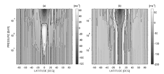
Figure 7: Zonal-mean zonal winds for Jupiter simulations with 3 times solar water abundance (left) and 10 times solar water abundance (right) at 1157 Earth days. The structures were time averaged for 231 Earth days. The solid and dashed lines depict eastward and westward winds, respectively, and the dotted lines represent zero speed. These lines only indicate the direction of the zonal winds. Note the development of equatorial superrotation in the 3-times-solar-water case and equatorial subrotation in the 10-times-solar-water case.

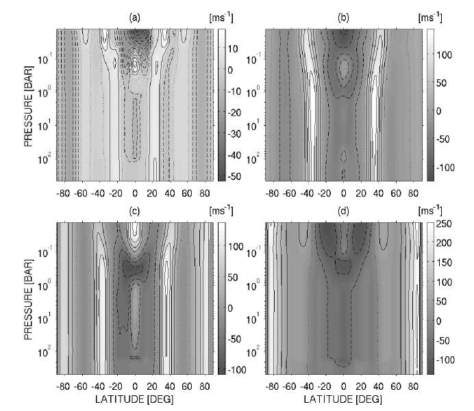
Figure 8: Zonal-mean zonal winds for Uranus/Neptune simulations with various abundances of water vapor at 2200 Earth days. The structures were time averaged for 231 Earth days. The solid and dashed lines depict eastward and westward winds, respectively, and the dotted lines represent zero speed. (a) 1 times the solar water abundance , line spacing is $\rm 5ms^{-1}$, (b) 3 times the solar water abundance, line spacing is $\rm 30ms^{-1}$, (c) 10 times the solar water abundance, line spacing is $\rm 30ms^{-1}$ and (d) 30 times the solar water abundance, line spacing is $\rm 50ms^{-1}$. Note that equatorial superrotation develops at low water abundances, but equatorial subrotation develops at 30 times solar water abundance.

To investigate the influence of water abundance on the circulation, and to shed light on what causes the differences between our Jupiter/Saturn and Uranus/Neptune cases (Fig. 2), we ran a series of simulations exploring a range of deep water-vapor abundances (Table 2). This is carried out simply by varying the value of the deep water abundance, $q_{\rm deep}$, adopted in our water-vapor source term $Q_{\rm deep}$. Figure 7 shows the results for Jupiter cases with 3 and 10 times solar water while Fig. 8 shows the results for Uranus/Neptune cases with 1, 3, 10, and 30 times solar water. Interestingly, we find in both cases that equatorial superrotation preferably forms at low water-vapor abundance while subrotation forms at high water-vapor abundance. For Jupiter, 3-times-solar water yields superrotation while 10-times-solar water produces subrotation. For Uranus/Neptune, solar water (panel a) produces a narrow superrotating jet centered at pressures of $\sim 100$–400 mbar; at 3-times-solar water (panel b), a local maximum in zonal wind still exists at that location, but its peak speeds are slightly subrotating. The ten-times-solar case (panel c) bucks the trend, developing superrotation in the lower stratosphere (pressures $<100\,$mbar). By 30 times solar, however, the structure becomes more barotropic and the equatorial jet direction is subrotating throughout. Nevertheless, the superrotation in our low-water-abundance Uranus/Neptune cases is weaker than that in our Jupiter/Saturn cases, which suggests that water abundance is not the only factor that controls the existence of superrotation in our simulations. We return to this issue in Section 3.2.

We also performed Saturn simulations with not only 5-times-solar water abundance (as seen in Fig. 2) but 10 and 20 times solar as well. All these cases developed multiple banded zonal jets at both low and high latitudes. The 5-times-solar Saturn case developed equatorial superrotation, with zonal-mean speeds reaching $\sim 150\rm\,m\,s^{-1}$ eastward, while the 10-times-solar and 20-times-solar cases developed equatorial subrotation with speeds reaching $-100\rm\,m\,s^{-1}$ or more westward near 1 bar. While our ability to produce superrotation in a Saturn case with 5-times-solar water is encouraging, Saturn’s water abundance is unknown and could easily be as high as 10 times solar (e.g., Mousis et al., 2009); moreover, even our superrotating case produced a superrotating jet much weaker and narrower than the observed jet (which extends from $30^{\circ}$N to $30^{\circ}$S latitude and reaches peak speeds of $\sim 400\rm\,m\,s^{-1}$). This disagreement could mean that Saturn’s equatorial jet does not fit into the framework discussed here, and that the observed jet results instead from a different mechanism. On the other hand, processes excluded here, including moist convection, evaporating precipitation, and realistic radiative transfer, will all affect the tropospheric static stability and thus could influence the eddy/mean-flow interactions that pump the equatorial jet. Definitely assessing whether Saturn’s equatorial jet can result from cloud-layer processes will thus require next-generation models that include these improvements.

Another trend that occurs in our simulations is that the mean jet speeds and jet widths increase as the deep water-vapor abundance is increased. As a result, simulations with less water tend to have more jets than simulations with greater water. This trend is most evident in our Uranus/Neptune cases in Fig. 8: the peak jet speed increases from $\sim 50\,{\rm m}\,{\rm sec}^{-1}$ to $250\,{\rm m}\,{\rm sec}^{-1}$ as water is increased from solar to 30 times solar, while the number of jets drops from seven to three over this same sequence. However, the case with 10-times-solar-water does not fit the trend well. It has 7 zonal jets, the same as our solar case, and its wind speeds are similar to that of our 3-times-solar case.

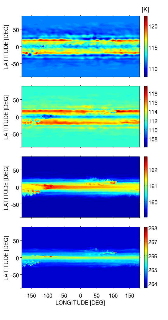
Figure 9: Global temperature maps for Jupiter simulation with 3 times the solar water abundance at 2315 Earth days. The pressure levels are, from top down, 0.1-bar level, 0.2-bar level, 0.9-bar level and 5-bar level.

Figure 9 shows the temperature structure in our nominal Jupiter simulation at pressures of 0.1, 0.2, 0.9, and 5 bars from top to bottom, respectively. The top two panels are in the lower stratosphere and upper troposphere; the third panel is near the top of the region with strong eddy accelerations, and the bottom panel is just above the water condensation level. Interestingly, in the deep regions where latent heating occurs (bottom two panels), the latitudinal temperature contrasts primarily occur within $\sim 20^{\circ}$ of the equator. In the simulations of Williams (2003c) and Lian and Showman (2008), equatorial superrotation developed only in the presence of large latitudinal temperature contrasts near the equator; this lead to a barotropic instability that pumped energy and momentum into the superrotating jet. In their simulations, these near-equatorial temperature gradients resulted from an ad hoc Newtonian heating profile. Here, however, these sharp near-equatorial temperature gradients develop naturally from the interaction of the moist convection with the large-scale flow. Despite this difference, the similarity of the resulting near-equatorial temperature profiles suggest that the superrotating jet-pumping mechanism identified by Williams (2003c) and Lian and Showman (2008) could be relevant here. In the upper troposphere and lower stratosphere, our Jupiter simulation develops a banded temperature pattern, with latitudinal temperature differences of $\sim 10\,$K, that bears some similarities to that observed on Jupiter and Saturn. Interestingly, the simulated equatorial zone is cold in the upper troposphere, consistent with observations of Jupiter and Saturn; this temperature structure is associated with the decay of the equatorial jet with altitude (see Fig. 7) via thermal-wind balance. Several regions of localized latent heating and eddy generation are visible in both hemispheres; Section 3.5 presents a detailed discussion of these features.

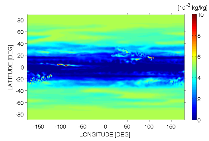
Figure 10: Global map of water-vapor mixing ratio for Jupiter simulation with 3 times the solar water abundance at 2315 Earth days. Shown at the 5-bar level.

Figure 10 depicts the distribution of water vapor at the 5-bar level for our nominal Jupiter simulation at the same time as the temperature plots shown in the previous figure. A zonally banded structure is evident, with low water vapor near the equator and intermediate values at mid-to-high latitudes. Localized regions of latent heating manifest as regions of high water vapor abundance near the equator and at $\sim 20^{\circ}$ latitude in both hemispheres (orange/red regions in the figure). While the connection between temperature and water vapor is visually evident (compare Figs. 10 and 9, bottom panel), scatter plots of temperature versus water-vapor mixing ratio at a given isobar show a great deal of scatter, indicating that no simple relationship connects the two quantities. Diagnostics of the mechanisms that determine the water and temperature distributions will be presented in a future paper.

3.2 What controls the equatorial flow

Among all our simulation results, the most interesting feature is that the direction and strength of equatorial flow vary with deep water abundance; eastward equatorial flow forms at low deep water abundance and westward equatorial flow forms at high deep water abundance. What causes this trend? Moreover, the planets in our simulations have different radii and rotation rates. Can these affect the formation of equatorial flow? Here we address these questions.

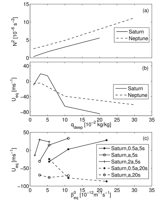
Figure 11: (a) Relation between $N^{2}$, where $N$ is Brunt Vaisala frequency in region deeper than 1 bar, and $q_{\rm deep}$ for Saturn and Neptune cases. Greater water abundance leads to greater static stability in the troposphere. (b) Relation between height-averaged equatorial wind and deep water abundance for Saturn and Neptune cases. Greater water abundance generally leads to stronger westward equatorial wind. (c) Relation between height-averaged equatorial wind and equatorial value of $\beta$, the gradient of Coriolis parameter (equal to $2\Omega/a$ at the equator) in Saturn-type cases varying the planetary rotation rate, radius, and deep water abundance. The relationship is complex (see text). Solid lines show 5 times solar and dashed lines show 20 times solar $q_{\rm deep}$. Each curve varies the rotation rate at a given $q_{\rm deep}$ and radius (between half and double Saturn’s actual radius, as marked in the legend), and different curves use different radii and/or $q_{\rm deep}$. All results are shown at 1157 Earth days. Table 2 lists all the cases shown here.

We performed additional test cases by varying the deep-water-vapor abundance, planetary radius, and planetary rotation rate (Table 2). By comparing the equatorial zonal wind, Brunt Vaisala frequency, and $\beta$, we seek to reveal the major factor that affects the trend. In the following discussion, the zonal wind is vertically averaged from the bottom to top of the simulated domain, while the Brunt-Vaisala frequency is vertically averaged from the bottom to 1 bar to exclude the large static stability in the stratosphere and thus better demonstrate the effects of latent heating in the troposphere. First, we vary the deep water abundance for Saturn and Neptune simulations using the nominal planetary radii and rotation rates; the results are shown in the top two panels of Fig. 11. Figure. 11(a) clearly shows that when the deep water abundance increases, the tropospheric Brunt-Vaisala frequency increases. Figure 11(b) confirms that larger deep water abundance (hence tropospheric static stability) makes the equatorial flow more westward. This correlation applies to both the Saturn and Neptune simulations (solid and dashed lines and dashed lines in Fig. 11, respectively) except the case of Saturn with 1-times-solar water abundance, in which the equatorial flow is very weak due to the low deep water abundance.

Although a clear correlation exists between greater deep water abundance and faster westward equatorial flow (Fig. 11b), the Neptune simulations exhibit a different dependence than the Saturn simulations. This suggests that other factors, such as planetary radius or rotation rate, play a role in controlling the equatorial jet speed. In an attempt to untangle these effects, we ran Saturn sensitivity studies that varied the planetary radius or rotation rate from nominal Saturn values but kept all other parameters fixed. Cases with deep water abundances of 5 and 20 times solar were explored. Figure 11(c) depicts the equatorial wind speed versus the equatorial value of $\beta$, the gradient of the Coriolis parameter (just $2\Omega/a$ at the equator). Solid lines denote the 5-times-solar cases while the dashed lines show the 20-times-solar cases. Different symbols denote different planetary radii and/or deep-water abundances; lines connect sequences of simulations performed at a given planetary radius and deep-water abundance but with differing rotation rate. At 5-times-solar water abundance, increasing the rotation rate (at constant planetary radius) makes the equatorial flow more eastward. However the situation reverses at 20-times-solar, where increasing the rotation rate either has minimal effect on the equatorial jet (for Saturn’s radius) or makes the jet more westward (for cases with half Saturn’s radius). At constant $\beta$ and water abundance, increasing the planetary radius makes the flow more eastward for our 5-times-solar-water cases but either has minimal effect or makes the equatorial flow more westward for our cases with 20-times-solar water.

In some cases, these dependences on radius and rotation rate can make the difference between whether the equatorial flow is eastward or westward. For example, the Saturn cases with 5-times-solar water all transition from westward to eastward equatorial flow as the rotation rate increases. Likewise, cases with 5-times-solar water and $\beta$ of 5–$10\times 10^{-12}\rm\,m\,sec^{-1}$ exhibit equatorial superrotation when performed at Saturn’s nominal radius but equatorial subrotation when performed at half Saturn’s radius.

To summarize our simulations, equatorial superrotation occurs only at intermediate water abundances; large deep water abundance instead promotes the development of equatorial subrotation for all cases explored. Everything else being equal, greater rotation rate and planetary radius promote equatorial superrotation when the water abundance is intermediate ($\sim 5$-times solar). The trends are less clear at high water abundance ($\sim 20$ times solar), but regardless of the details our high-water-abundance cases all subrotate. Taken together, the sensitivity studies described here show that the equatorial superrotation in our successful Jupiter and Saturn simulations (e.g., as shown in Fig. 2) is enabled not only by the low-to-intermediate water abundance adopted in those cases but also by the large planetary radius and faster rotation rates of Jupiter and Saturn relative to Uranus and Neptune. Loss of any one of those factors would promote weaker superrotation or even a transition to equatorial subrotation. This is consistent with the fact that the Uranus/Neptune cases shown in Fig. 8 exhibit only rather weak superrotation (relative to the Jupiter/Saturn cases) even when the water abundance is 1, 3, or 10 times solar.

3.3 What drives the jets in weather layer

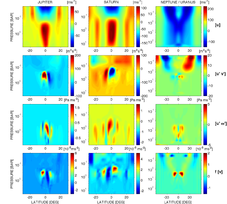
Figure 12: Eddy fluxes and accelerations for Jupiter simulation with 3 times solar water (left column), Saturn simulation with 5 times solar water (middle column), and Uranus/Neptune simulation with 30 times solar water (right column). Top row: zonal-mean zonal winds. Second row: horizontal flux of eastward momentum, $[{\overline{u^{\prime}v^{\prime}}}]+[{\overline{u}}^{*}{\overline{v}}^{*}]$. Positive means northward flux and negative means southward flux. Third row: vertical flux of eastward momentum $[{\overline{u^{\prime}\omega^{\prime}}}]+[{\overline{u}}^{*}{\overline{\omega}}^{*}]$. Positive means downward flux and negative means upward flux. Bottom row: Coriolis acceleration on the mean-meridional circulation, $f[{\overline{v}}]$. All quantities are averaged over 231 Earth days ending at day 578, 1600, and 578 Earth days, respectively, for the Jupiter, Saturn, and Uranus/Neptune cases.

Our Jupiter, Saturn, and Uranus/Neptune simulations show that the zonal jets are predominantly driven by eddy and Coriolis acceleration. We use the total acceleration of the terms on the right side of Eq. 9 to characterize the main driving forces on the zonal flow, focusing here on the mid- and low-latitude regions. Figure 12 shows the zonal-mean zonal wind (top row), horizontal eddy-momentum flux $[{\overline{u^{\prime}v^{\prime}}}]+[{\overline{u}}^{*}{\overline{v}}^{*}]$ (second row), the vertical eddy-momentum flux $[{\overline{u^{\prime}\omega^{\prime}}}]+[{\overline{u}}^{*}{\overline{\omega}}^{*}]$ (third row), and Coriolis acceleration $f[\overline{v}]$ (bottom row). Three cases are shown — our 3-times-solar water Jupiter case (left column), 5-times-solar Saturn case (middle row), and 30-times-solar Uranus/Neptune case (right column). The Jupiter and Saturn cases exhibits equatorial superrotation while the Uranus/Neptune case exhibits equatorial subrotation.

Figure 12 shows that the horizontal eddy terms, vertical eddy terms, and Coriolis accelerations all play important roles in the maintenance of the zonal winds. In particular, for our Jupiter and Saturn cases, there are strong equatorward fluxes of eastward momentum at pressures of $\sim 0.2$–$1\,$bar and latitudes of $\sim 10^{\circ}$S to $10^{\circ}$N. These imply an eastward acceleration that helps to maintain the superrotating equatorial jet. They additionally cause a westward acceleration at latitudes of $\sim 10^{\circ}$N and S, where a divergence in horizontal flux occurs. In contrast, our Uranus/Neptune case exhibits strong poleward fluxes of eastward momentum at pressures $<1\,$bar and latitudes equatorward of $\sim 40^{\circ}$. These fluxes induce westward equatorial acceleration, which maintains the strong westward equatorial flows at low pressure. A weaker version of the same phenomenon occurs in the Jupiter and Saturn cases, which helps explain the westward equatorial stratospheric flow near the top of the model (pressures $<0.1\,$bar) in those cases. Nevertheless, the Uranus/Neptune case also shows a localized region (from $1$–$2\,$bars and latitudes $\sim 10^{\circ}$S to $10^{\circ}$N) where eastward momentum fluxes (albeit weakly) toward the equator, leading to an eastward equatorial acceleration. This relates to the fact that the westward jet, once formed, weakens slightly between $\sim 100$ and $1000\,$days (compare second and third rows of Fig. 4). Interestingly, all three cases also show an overall downward eddy flux of eastward momentum in the equatorial regions underlying the region of horizontal eddy fluxes. In the Jupiter/Saturn cases, this term causes an acceleration counteracting that associated with horizontal eddy-flux convergence and helps to explain why the eastward jets penetrate to pressures $>10\,$bars despite the fact that the horizontal eddy fluxes are confined primarily to pressures $<1\,$bar. The Coriolis accelerations (bottom row) show localized regions of eastward acceleration centered just off the equator in all three cases (at pressures 0.2–$1\,$bar for Jupiter/Saturn and $\sim 2$–$8\,$bars for Uranus/Neptune) resulting from the effects of a meridional circulation cell near the equator. In all three cases, this acts to counteract a westward acceleration associated with horizontal eddy flux convergence at the same location.

An estimate of magnitudes shows that all these acceleration terms are important. For example, focusing on Jupiter and Saturn, the Coriolis acceleration reaches peak values up to a few $\times 10^{-5}\rm\,m\,s^{-2}$ (Fig. 12, bottom row). The acceleration caused by horizontal eddy flux convergence is minus the gradient of $[{\overline{u^{\prime}v^{\prime}}}]+[{\overline{u}}^{*}{\overline{v}}^{*}]$, which is approximately the difference in this quantity over a relevant length scale. Figure 12, second row, shows that the peak difference in $[{\overline{u^{\prime}v^{\prime}}}]+[{\overline{u}}^{*}{\overline{v}}^{*}]$ is $\sim 200\rm\,m^{2}\,s^{-2}$ and occurs over a latitudinal length scale of $\sim 8000\,$km, implying an acceleration of $\sim 3\times 10^{-5}\rm\,m\,s^{-2}$. Likewise from Figure 12, third row, the peak difference in $[{\overline{u^{\prime}\omega^{\prime}}}]+[{\overline{u}}^{*}{\overline{\omega}}^{*}]$ is $\sim 1\rm\,Pa\,m\,s^{-2}$, which occurs over a pressure interval of $\sim 10^{5}\,$Pa, implying an acceleration of $\sim 10^{-5}\rm\,m\,s^{-2}$.

For all these cases, there are partial cancellations between the individual terms that generally leads to a net acceleration smaller than the magnitude of the dominant individual terms. More than $\sim 5$–$10^{\circ}$ away from the equator, there is an anticorrelation between the Coriolis acceleration and acceleration due to horizontal eddy convergence, leading to a significant cancellation between these terms. Accelerations due to vertical eddy convergence play only a small role in these regions because the ratio of accelerations due to vertical and horizontal eddy convergences tends to scale as the Rossby number, which is small away from the equator. However, near the equator the Coriolis acceleration is weak, and within $\sim 3$–$5^{\circ}$ latitude of the equator, the dominant cancellation is between the horizontal and vertical eddy terms for Jupiter, Saturn and Uranus/Neptune. Because of these partial cancellations, the net acceleration is relatively small once the jets have spun up, leading to only gradual change in the zonal-jet speeds over time.

3.4 Comparison between simulations and observations

Now we compare our simulated jet profiles to the observed jet profiles and their stability. Jupiter and Saturn’s cloud-level winds violate the barotropic stability criterion (Ingersoll et al., 1981)

$$\frac{\partial^{2}[u]}{\partial{y^{2}}}<\beta.$$ (10)

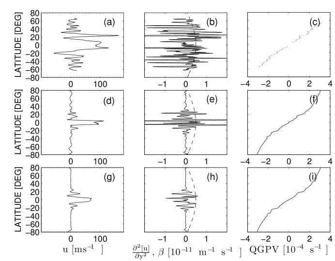
Figure 13: Zonal-mean zonal winds (left column), curvature of zonal-mean-zonal winds $\partial^{2}[u]/\partial y^{2}$ with northward distance $y$ (middle column) at $\sim 0.6\,$bars, and zonal-mean quasigeostrophic potential vorticity (right column) at $\sim 0.12\,$bars. In the middle column, $\beta$ is included as a dashed curve for comparison. Top row (a, b, and c) shows Voyager 2 measurements; winds are from Limaye (1986) and PV is from Read et al. (2006). Middle row (d, e, and f) shows the zonal winds properties at $163^{\circ}$ east in our Jupiter-type simulation with 3 times solar water abundance at 2200 Earth days. Bottom row (g, h, and i) shows the zonal mean zonal winds properties in our Jupiter simulation at 2200 Earth days.

The observed winds also violate the Charney-Stern criterion which states that jets are stable if their potential vorticity profile is monotonic in latitude (Dowling, 1995). Figure 13 shows the comparison between observed and simulated jet profiles for Jupiter. The top row shows observations. The middle row shows simulated winds at $\rm 163^{\circ}$ longitude. The bottom row shows zonal-mean simulated zonal winds. The wind profile shown is at $\rm\sim 0.6\,bars$ and potential vorticity shown is at $\rm\sim 0.12\,bars$. We calculate quasi-geostrophic potential vorticity $q_{G}$ following Read et al. (2006):

$$q_{G}=f+\zeta-f{\partial\over\partial p}\left[{p\Delta T(\lambda,\phi,p)\over s(p)T_{a}(p)}\right],$$ (11)

where $\zeta$ is relative vorticity calculated on isobars, $T_{a}(p)=\langle{T(\lambda,\phi,p)}\rangle$ is the horizontal mean temperature calculated on isobars, $\Delta{T(\lambda,\phi,p)}=T(\lambda,\phi,p)-T_{a}(p)$ is deviation of temperature from its horizontal mean, and $s(p)$ is a stability factor defined as

$$s(p)=-{\partial{\langle{\ln(\theta)}\rangle}\over{\partial{\ln p}}}.$$ (12)

where $\langle\theta\rangle$ is the horizontal mean potential temperature calculated on isobars.

Our Jupiter simulation with 3 times solar water abundance shows that the zonal winds are slightly weaker and the equatorial superrotation is narrower than observed. The zonal winds in some longitudinal cross sections violate the barotropic and Charney-Stern stability criteria. Figure 13(e) shows that the wind curvature $\partial^{2}[u]/{\partial{y^{2}}}$ in a longitudinal slice (here arbitrarily chosen as $\rm 163^{\circ}$ east) exceeds $3\beta$ at some latitudes. At the same time, the latitudinal gradient of quasigeostrophic potential vorticity changes sign at many places, as shown in Fig. 13(f). The zonal-mean zonal wind, however, has a much weaker violation of the barotropic stability criterion. It only exceeds $\beta$ at $\rm\pm 20^{\circ}$ in latitude.

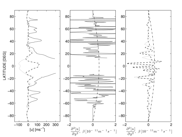
Figure 14: Saturn zonal-mean zonal winds (left), curvature of observed zonal-mean-zonal winds $\partial^{2}[u]/\partial y^{2}$ with northward distance $y$ (middle) and curvature $\partial^{2}[u]/\partial y^{2}$ of our Saturn simulations (right). In all panels, solid curve is Saturn observations from Voyager, dashed curve is Saturn simulation with 5 times solar water, and dotted curve is Saturn simulation with 10 times solar water. In the middle and right panels, $\beta$ is included as a dot-dashed curve for comparison. Simulation results are shown at 1 bar and observations are also roughly at 1 bar.

Figure 14 compares observations and simulations for Saturn. Zonal-mean zonal wind profiles are shown on the left, with Voyager observations (solid), our Saturn 5-times-solar-water simulation (dashed), and our Saturn 10-times-solar-water simulation (dotted). The middle and right panels show $\partial^{2}[u]/\partial y^{2}$ for the observations and our simulations, respectively. As can be seen, our simulations produce winds with speeds smaller than observed, especially in the equatorial jet. Interestingly, our Saturn simulation with 5-times-solar water, which produces equatorial superrotation of $150\rm\,m\,s^{-1}$, violates the barotropic stability criterion at some latitudes. In contrast, our Saturn simulation with 10-times-solar water, which produces equatorial subrotation, satisfies the barotropic stability criterion at all latitudes.

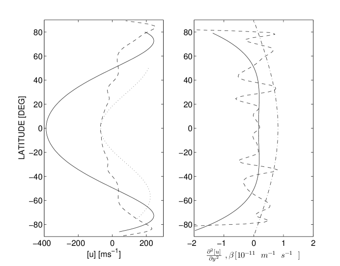
Figure 15: Zonal-mean zonal winds (left column) and curvature of zonal-mean-zonal winds $\partial^{2}[u]/\partial y^{2}$ with northward distance $y$ (right column) at $\sim 1\,$bar. In the right column, $\beta$ is included as a dot-dashed curve for comparison. The solid line shows Voyager 2 measurements of Neptune winds; winds are from Sromovsky et al. (1993). The dashed line shows the zonal winds properties in our Neptune-type simulation with 30 times solar water abundance at 2200 Earth days. The dotted line shows HST measurement of Uranus winds; winds are from Hammel et al. (2001).

We also compare jet profiles in our Uranus/Neptune simulation with 30 times solar water abundance to observations. Figure 15 shows the observed winds on Uranus and Neptune and simulated winds at $\rm\sim 1\,$ bar. Our simulated zonal winds share similarities with the observed winds, especially the three-jet feature with a subrotating equator and high-latitude eastward jets. Comparing to the zonal winds on Neptune, the equatorial subrotation in our simulation achieves speed of $\rm 100\,m\,s^{-1}$ which is weaker than the observed $\rm 400\,m\,s^{-1}$; the polar eastward winds, though appearing at too high a latitude, have similar strength as observed. On the other hand, the simulated jets have similar strength as both westward and eastward jets on Uranus. However, the westward jet on Uranus is much narrower than that in our simulation and on Neptune. Furthermore, Uranus has eastward jets peaking in the mid-latitudes rather than near the poles as in our simulation. Interestingly, zonal winds in our simulation violate the barotropic stability criterion while those in observations do not.

Even though the zonal jets in our simulations violate the barotropic stability criterion, the time-averaged jets are still stable which suggests a stable configuration between the eddies and zonal jets. This stable configuration also exists in our previous simulations (Lian and Showman, 2008).

3.5 Morphology of eddies generated by large-scale latent heating

In our Jupiter and Saturn simulations, large-scale latent heating and rising motion often become concentrated into localized regions, leading to the development of small ($\sim$3000–10,000-km diameter) warm-core eddies that play a key role in driving the flow. These events share similarities with storm clouds observed on Jupiter and Saturn, so here we describe them in detail. For lack of a better word, we call these events “storms” but remind the reader that our model lacks non-hydrostatic motions and sub-grid-scale parameterizations of true moist convection.

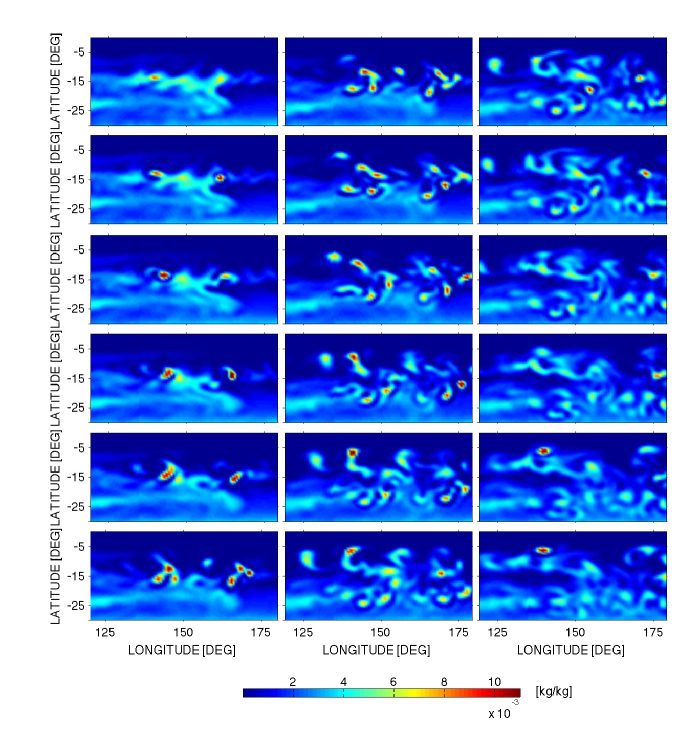
Figure 16: A zoom-in showing evolution of water-vapor mixing ratio at the 5-bar level in a portion of the domain centered around a moist-convection event for our Jupiter simulation with 3 times the solar water abundance. Left column (from top down) starts from 1185 Earth days and ends at 1199 Earth days. Middle column (from top down) starts from 1201.8 Earth days and ends at 1215.8 Earth days. Right column (from top down) starts from 1218.6 Earth days and ends at 1232.6 Earth days. The time interval between two adjacent time frames in a column is 2.8 Earth days.

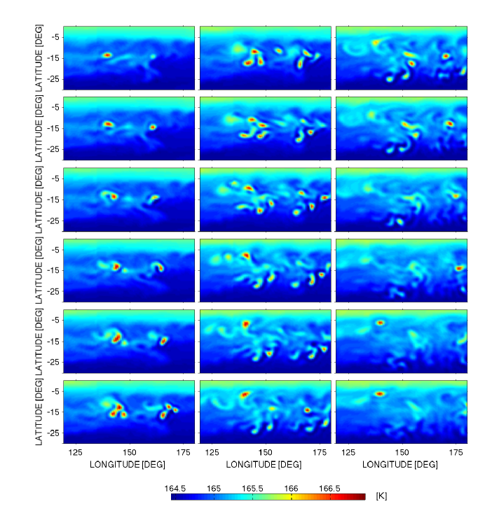
Figure 17: Same as Fig. 16 but shows potential temperature at the 5-bar level.

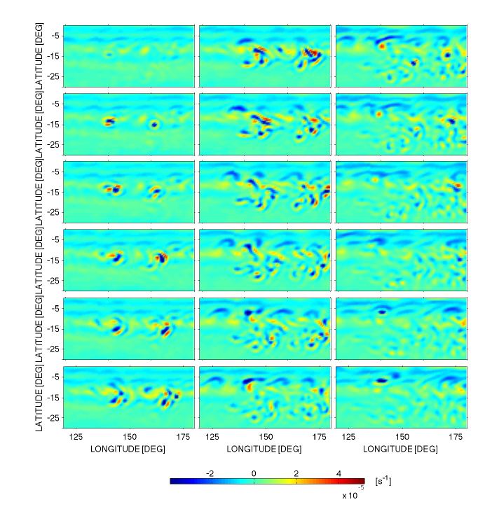
Figure 18: Same as Fig. 16 but shows relative vorticity at the 5-bar level. Blue is cyclonic and red is anticyclonic.

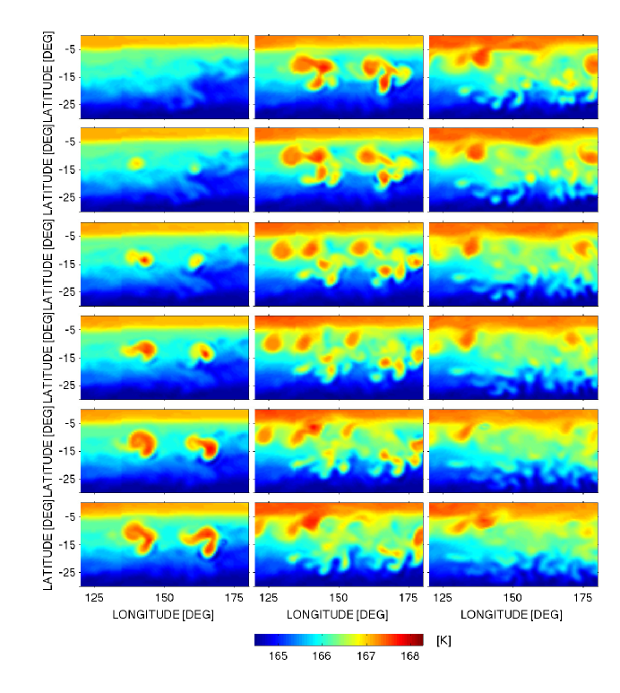
Figure 19: Same as Fig. 16 but shows potential temperature at the 0.9-bar level.

Figures 16–19 depict time sequences that zoom into the region around one such event; the sequences start at the upper left and move first downward and then right in 2.8-Earth-day intervals. Figure 16, which depicts the water-vapor mixing ratio, shows the active storms as bright red regions with much greater water abundance than the surroundings. Figure 17 demonstrates that these regions of high humidity are warmer than the surroundings, which is the direct result of latent heating in the rising air. Plots of vertical velocity (not shown) show that these warm, moist regions are ascending. Figure 18 depicts the relative vorticity; a careful comparison with Figs. 16–17 shows that, at the base of the storms near 5 bars, the hot, moist ascending regions generally exhibit cyclonic relative vorticity, which results from the Coriolis acceleration on the air converging horizontally into the base of the storm at that pressure. Although the storms are extremely dynamic, they are self-generating and can last for tens of days.

Interestingly, the cyclonic regions at the base of the updrafts (blue in Fig. 18) typically co-exist with one or more localized anticyclonic regions (red in Fig. 18), which are locations where air descends, horizontally diverges, and thus spins up anticyclonically. The existence of descending regions in proximity to the ascending storm centers results from mass continuity; as air rises in an active storm center, continuity demands descent in the surrounding environment. A similar phenomenon occurs around storms on Earth; theoretical solutions show that such descent is typically confined to regions within a deformation radius of the ascending storm center (Emanuel, 1994, pp. 329-333). This result can explain the close proximity of the ascending and descending regions in our simulations, as well as the fact that Jovian thunderstorms are often observed next to localized regions that are clear down to the 4-bar level or deeper (Banfield et al., 1998; Gierasch et al., 2000).

The behavior near the tops of the simulated storms differs significantly from that near their bases. This is illustrated in Fig. 19, which shows the temperature at 0.9 bars for the same storm event depicted in Figs. 16–18. Hot regions in Fig. 17 generally correlate with hot regions in Fig. 19, which results from the fact that the hot, moist air at 5 bars generally continues rising until reaching altitudes at and above the 1-bar level. However, the localized hot regions at 0.9 bars are much larger than at 5 bars. This presumably results from the horizontal divergence that occurs near the storm top, which spreads the hot regions out into “anvils” whose horizontal extent significantly exceeds that at the base of the storm. Conversely, we speculate that the horizontal convergence at the storm base helps to keep the hot regions horizontally confined at that pressure. The horizontal divergence near the storm top also implies that the storms generate regions of anticyclonic vorticity as seen at 1 bar (not shown). This is consistent with observations of Jovian thunderstorms, which generally also develop anticyclonic vorticity at the ammonia cloud level (Gierasch et al., 2000).

The simulated storms exhibit a complex evolution. The storms often appear in clusters with several simultaneously active centers (Figs. 16–19); this could occur because the large-scale environment in that region is primed for storm generation, but it also suggests that the storms may self-interact in a way that can trigger new storms. As shown in Figure 19, active storm centers sometimes shed warm-core vortices that have lifetimes up to tens of days and propagate downstream away from the active storm region. Fig. 17 exhibits several examples where features appear to “die out” at 5 bars, but a comparison with Fig.19 shows that, in several cases, the features have not decayed but instead have simply ascended to the $\sim 1$-bar level. Indeed, several of the warm-core vortices visible in Fig. 19 have essentially no signature at 5 bars, indicating that these vortices are no longer fed by upward motion from near the water-condensation level.

Importantly, the properties of our simulated storms — including their size, amplitude, lifetime, and morphology — are self-consistently generated by the dynamics and are therefore predictions of our model. This contrasts with previous studies attempting to model the effect of moist convection on the large-scale flow (Li et al., 2006; Showman, 2007), which introduced mass pulses by hand to represent storms, and which imposed the size, shape, amplitude, and lifetime of the storms as free parameters.

Despite the lack of small-scale convective dynamics in our model, our simulated storms show an encouraging resemblance to the evolution of cloud morphology in real moist-convection events on Jupiter and Saturn. On Jupiter, individual storm clouds often last for up to several days and expand to diameters up to $\sim 1000$–$3000\,$km (Gierasch et al., 2000; Porco et al., 2003; Sánchez-Lavega et al., 2008), although rare events sometimes reach sizes of $10,000\,$km or more (Hueso et al., 2002) and lifetimes up to 10 days (Porco et al., 2003). On Saturn, storms lasting tens of days have been observed by Voyager and Cassini (Sromovsky et al., 1983; Porco et al., 2005; Dyudina et al., 2007); individual active storm centers reach $\sim 2000\,$km diameters within an active storm complex up to $\sim 6000\,$km across. The observed clouds are probably large-scale anvils fed by numerous individual convective storms that become spatially organized, analogous to “mesoscale convective complexes” on Earth (Gierasch et al., 2000). As already described, the rapid expansion and generation of anticyclonic vorticity near the tops of our simulated storms and the close proximity of ascending active storm centers to subsiding regions are consistent with observations of jovian storms, although our storm sizes and lifetimes are somewhat too large. The creation of (generally short-lived) vortices from latent heating, as occurs in our simulations, has not been clearly observed on Jupiter, but storm-generated vortices have tentatively been captured in Cassini images on Saturn (Porco et al., 2005; Dyudina et al., 2007). A similar phenomenon was obtained in the shallow-water simulations of Showman (2007).

It is worth re-iterating that our simulations adopt local hydrostatic balance and thus cannot capture the strong vertical accelerations associated with convectively unstable motions and lightning generation. At present, such phenomena can only be resolved by regional-scale non-hydrostatic models (e.g. Yair et al., 1995; Hueso and Sánchez-Lavega, 2001), although the effects of such convective motions on the large-scale flow could potentially be represented in large-scale models using a cumulus parameterization. The large horizontal dimensions of observed jovian/saturnian storm anvil clouds, and the qualitative similarity of our results to the observed storms, supports the possibility that such efforts could prove fruitful in attempting to explain observations of storm-cloud evolution on Jupiter and Saturn.

4 Conclusion

We presented global, three-dimensional numerical models to simulate the formation of zonal jets by large-scale latent heating on the giant planets. These models explicitly include water vapor and its condensation and the resulting latent heating. We find that latent heating can naturally produce banded zonal jets similar to those observed on the giant planets. Our Jupiter and Saturn simulations develop $\rm\sim 20$ zonal jets and Uranus/Neptune simulations develop $\rm 3-7$ zonal jets depending on the water abundance. The jet spacing is consistent with Rhines scale $\pi(2U/\beta)^{1/2}$. The zonal jets in our simulations produce modest violations of the barotropic and Charney-Stern stability criteria at some latitudes.

In our simulations, condensation of water vapor releases latent heat and produces baroclinic eddies. These eddies interact with the large-scale flow and the $\beta$ effect to pump momentum up-gradient into the zonal jets. At the same time, a meridional circulation develops whose Coriolis acceleration counteracts the eddy accelerations in the weather layer. This near-cancellation of eddy and Coriolis accelerations leads to slow evolution of the zonal jets and maintains the steadiness of zonal jets in the presence of continual forcing. Such a process was suggested by Showman et al. (2006) and Del Genio et al. (2007) and occurred also in the simulations of Showman (2007) and Lian and Showman (2008).

Our simulations also produce equatorial superrotation for Jupiter and Saturn and subrotation for Uranus and Neptune. Although a number of previous attempts have been made to produce superrotation on Jupiter/Saturn and subrotation on Uranus/Neptune, previous models have generally lacked an ability to produce both superrotation on Jupiter/Saturn and subrotation on Uranus/Neptune without introducing ad hoc forcing or tuning of model parameters. Ours is the first study to naturally produce such dual behavior, without tuning, within the context of a single model. Although the speeds of the superrotation and subrotation are weaker than observed, our simulations provide a possible mechanism to explain the dichotomy in equatorial-jet direction between the gas giants (Jupiter/Saturn) and ice giants (Uranus/Neptune) within the context of a single model. In our simulations, the strength, scale, and direction of the equatorial flow are strongly affected by the abundance of water vapor as well as by the planetary radius and rotation rate. Equatorial superrotation preferably forms in simulations with modest water vapor abundance and is further promoted by large planetary radii and fast rotation rates, as occur at Jupiter and Saturn. In contrast, high water abundance leads to equatorial subrotation regardless of the planetary radius and rotation rate explored here. In this picture, the dichotomy in the equatorial jet direction between the gas and ice giants would result from a combination of the faster rotation rates, larger radii, and probable lower water abundances on Jupiter/Saturn relative to those on Uranus/Neptune.

Despite this encouraging result, Saturn poses a possible difficulty with this picture. Our Saturn simulations generated equatorial superrotation when the water abundance is five times solar but equatorial subrotation when it is ten times solar. Saturn’s actual water abundance is unknown but could easily lie anywhere within this range. Moreover, even our five-times-solar Saturn case produced a superrotation that is much weaker and narrower than observed — about $120\rm\,m\,s^{-1}$ in the simulation versus $\sim 400\rm\,m\,s^{-1}$ on the real planet. (The equatorial jet in our Jupiter simulations is also too narrow, although the discrepancy is less severe.) However, a variety of processes excluded here (e.g., cloud microphysics, realistic radiative transfer, and moist convection) could significantly affect the jet profile. Future investigations that include these effects are needed before a definite assessment can be made.

Consistent with our earlier work, we again find that our simulations generate deep barotropic jets despite the localization of the eddy accelerations to the weather layer (pressures less than $\sim 7\,$bars in our Jupiter simulations, for example). In some simulations, the deep jets have similar strength as the winds in weather layer. The mechanism that forms the deep jets is similar to the mechanism we previously identified (Lian and Showman, 2008; Showman et al., 2006). However, these deep jets are affected by the redistribution of water vapor, which makes the diagnostics very complicated in the present case.

Our simulations successfully produce the large-scale dynamic features on Jupiter and Uranus/Neptune under the effect of large-scale latent heating. However, our simulations lack long-lived vortices such as the Great Red Spot on Jupiter and Great Dark Spot on Neptune. We also ignore the precipitation and re-evaporation of condensates and use an idealized radiative cooling scheme. The grid resolution in our simulations is relatively low for resolving the mesoscale moist convection events which have typical horizontal scales of $1000$ kilometers (Little et al., 1999; Porco et al., 2003). Future models can include cloud physics, a sub-grid-scale parameterization of cumulus convection, a more realistic radiative transfer scheme, and explore the coupling between the deep interior and the weather-layer processes identified here.

5 Acknowledgement

This research was supported by NASA Planetary Atmospheres grant NNG06GF28G to APS.

Figure 3: Snapshots of zonal winds at 0.9 bars for our Jupiter simulation with 3 times the solar water abundance. The four rows, from top down, give the state at 3, 55, 116, 578, 1157 and 2315 Earth days. The left column shows the zonal wind over the full globe in a rectangular projection. The middle column gives the zonal wind profile at longitude $\rm-176.8^{\circ}$ (black line) and $\rm 0^{\circ}$ (red line). The right column is zonal-mean zonal wind.

References

- Arakawa (2004) Arakawa, A., Jul. 2004. The Cumulus Parameterization Problem: Past, Present, and Future. Journal of Climate 17, 2493–2525.
- Aurnou et al. (2007) Aurnou, J., Heimpel, M., Wicht, J., 2007. The effects of vigorous mixing in a convective model of zonal flow on the ice giants. Icarus 190, 110–126.
- Aurnou and Olson (2001) Aurnou, J. M., Olson, P. L., 2001. Strong zonal winds from thermal convection in a rotating spherical shell. Geophys. Res. Lett.28, 2557–2560.
- Baines et al. (1995) Baines, K. H., Hammel, H. B., Rages, K. A., Romani, P. N., Samuelson, R. E., 1995. Clouds and aerosols in the atmosphere of Neptune. In Neptune and Triton (Ed. by D. P. Cruikshank, University of Arizona Press), 489–546.
- Baines et al. (2009) Baines, K. H., Momary, T. W., Fletcher, L. N., Showman, A. P., Roos-Serote, M., Brown, R. H., Buratti, B. J., Clark, R. N., Nicholson, P. D., 2009. Saturn’s north polar cyclone and hexagon at depth revealed by Cassini/VIMS. Planet. Space Sci. (submitted).
- Banfield et al. (1998) Banfield, D., Gierasch, P. J., Bell, M., Ustinov, E., Ingersoll, A. P., Vasavada, A. R., West, R. A., Belton, M. J. S., 1998. Jupiter’s Cloud Structure from Galileo Imaging Data. Icarus 135, 230–250.
- Barcilon and Gierasch (1970) Barcilon, A., Gierasch, P., 1970. A Moist, Hadley Cell Model for Jupiter’s Cloud Bands. Journal of Atmospheric Sciences 27, 550–560.
- Borucki and Williams (1986) Borucki, W. J., Williams, M. A., 1986. Lightning in the Jovian water cloud. J. Geophys. Res. 91, 9893–9903.
- Campin et al. (2004) Campin, J.-M., Adcroft, A., Hill, C., Marshall, J., 2004. Conservation of properties in a free-surface model. Ocean Modelling 6, 221–244.
- Cho and Polvani (1996a) Cho, J. Y.-K., Polvani, L. M., 1996a. The morphogenesis of bands and zonal winds in the atmospheres on the giant outer planets. Science 8 (1), 1–12.
- Cho and Polvani (1996b) Cho, J. Y.-K., Polvani, L. M., 1996b. The emergence of jets and vortices in freely evolving, shallow-water turbulence on a sphere. Physics of Fluids 8, 1531–1552.
- Christensen (2001) Christensen, U. R., 2001. Zonal flow driven by deep convection in the major planets. Geophys. Res. Lett.28, 2553–2556.
- Del Genio et al. (2007) Del Genio, A. D., Babara, J. M., Ferrier, J., Ingersoll, A. P., West, R. A., Vasavada, A. R., Spitale, J., Porco, C. C., 2007. Saturn eddy momentum fluxes and convection: first estimates from Cassini images. Icarus, in press.
- Del Genio and McGrattan (1990) Del Genio, A. D., McGrattan, K. B., 1990. Moist convection and the vertical structure and water abundance of Jupiter’s atmosphere. Icarus 84, 29–53.
- Dowling (1995) Dowling, T. E., 1995. Dynamics of Jovian atmospheres. Ann. Rev. Fluid Mech. 27, 293–334.
- Dyudina et al. (2007) Dyudina, U. A., Ingersoll, A. P., Ewald, S. P., Porco, C. C., Fischer, G., Kurth, W., Desch, M., Del Genio, A., Barbara, J., Ferrier, J., 2007. Lightning storms on Saturn observed by Cassini ISS and RPWS during 2004 2006. Icarus 190, 545–555.
- Dyudina et al. (2002) Dyudina, U. A., Ingersoll, A. P., Vasavada, A. R., Ewald, S. P., The Galileo SSI Team, 2002. Monte Carlo Radiative Transfer Modeling of Lightning Observed in Galileo Images of Jupiter. Icarus 160, 336–349.
- Emanuel (1994) Emanuel, K. A., 1994. Atmospheric Convection. Oxford Univ. Press, New York.
- Emanuel and Raymond (1993) Emanuel, K. A., Raymond, D., 1993. The Representation of Cumulus Convection in Numerical Models. American Meteorological Society, Boston.
- Fegley et al. (1991) Fegley, B. J., Gautier, D., Owen, T., Prinn, R. G., 1991. Spectroscopy and chemistry of the atmosphere of Uranus. In Uranus (Ed. by J. Bergstrahl, University of Arizona Press), 147–203.
- Flasar et al. (2005) Flasar, F. M., Achterberg, R. K., Conrath, B. J., Pearl, J. C., Bjoraker, G. L., Jennings, D. E., Romani, P. N., Simon-Miller, A. A., Kunde, V. G., Nixon, C. A., Bézard, B., Orton, G. S., Spilker, L. J., Spencer, J. R., Irwin, P. G. J., Teanby, N. A., Owen, T. C., Brasunas, J., Segura, M. E., Carlson, R. C., Mamoutkine, A., Gierasch, P. J., Schinder, P. J., Showalter, M. R., Ferrari, C., Barucci, A., Courtin, R., Coustenis, A., Fouchet, T., Gautier, D., Lellouch, E., Marten, A., Prangé, R., Strobel, D. F., Calcutt, S. B., Read, P. L., Taylor, F. W., Bowles, N., Samuelson, R. E., Abbas, M. M., Raulin, F., Ade, P., Edgington, S., Pilorz, S., Wallis, B., Wishnow, E. H., 2005. Temperatures, Winds, and Composition in the Saturnian System. Science 307, 1247–1251.
- Gierasch (1976) Gierasch, P. J., 1976. Jovian meteorology - Large-scale moist convection. Icarus 29, 445–454.
- Gierasch et al. (2000) Gierasch, P. J., Ingersoll, A. P., Banfield, D., Ewald, S. P., Helfenstein, P., Simon-Miller, A., Vasavada, A., Breneman, H. H., Senske, D. A., A4 Galileo Imaging Team, 2000. Observation of moist convection in Jupiter’s atmosphere. Nature403, 628–630.
- Glatzmaier et al. (2008) Glatzmaier, G. A., Evonuk, M., Rogers, T. M., 2008. Differential rotation in giant planets maintained by density-stratified turbulent convection. ArXiv e-prints 806.
- Godfrey (1988) Godfrey, D. A., Nov. 1988. A hexagonal feature around Saturn’s North Pole. Icarus 76, 335–356.
- Gurnett et al. (1990) Gurnett, D. A., Kurth, W. S., Cairns, I. H., Granroth, L. J., 1990. Whistlers in Neptune’s magnetosphere - Evidence of atmospheric lightning. J. Geophys. Res. 95, 20967–20976.
- Hammel et al. (2001) Hammel, H. B., Rages, K., Lockwood, G. W., Karkoschka, E., de Pater, I., 2001. New Measurements of the Winds of Uranus. Icarus 153, 229–235.
- Heimpel and Aurnou (2007) Heimpel, M., Aurnou, J., 2007. Turbulent convection in rapidly rotating spherical shells: A model for equatorial and high latitude jets on Jupiter and Saturn. Icarus 187, 540–557.
- Heimpel et al. (2005) Heimpel, M., Aurnou, J., Wicht, J., 2005. Simulation of equatorial and high-latitude jets on Jupiter in a deep convection model. Nature 438, 193–196.
- Huang and Robinson (1998) Huang, H.-P., Robinson, W. A., 1998. Two-Dimensional Turbulence and Persistent Zonal Jets in a Global Barotropic Model. Journal of Atmospheric Sciences 55, 611–632.
- Hueso and Sánchez-Lavega (2001) Hueso, R., Sánchez-Lavega, A., 2001. A Three-Dimensional Model of Moist Convection for the Giant Planets: The Jupiter Case. Icarus 151, 257–274.
- Hueso et al. (2002) Hueso, R., Sánchez-Lavega, A., Guillot, T., 2002. A model for large-scale convective storms in Jupiter. Journal of Geophysical Research (Planets) 107, 5075–+.
- Iacono et al. (1999) Iacono, R., Struglia, M. V., Ronchi, C., 1999. Spontaneous formation of equatorial jets in freely decaying shallow water turbulence. Physics of Fluids 11, 1272–1274.
- Ingersoll et al. (1981) Ingersoll, A. P., Beebe, R. F., Mitchell, J. L., Garneau, G. W., Yagi, G. M., Muller, J.-P., 1981. Interaction of eddies and mean zonal flow on Jupiter as inferred from Voyager 1 and 2 images. J. Geophys. Res. 86, 8733–8743.
- Ingersoll et al. (2004) Ingersoll, A. P., Dowling, T. E., Gierasch, P. J., Orton, G. S., Read, P. L., Sánchez-Lavega, A., Showman, A. P., Simon-Miller, A. A., Vasavada, A. R., 2004. Dynamics of Jupiter’s atmosphere. Jupiter. The Planet, Satellites and Magnetosphere, pp. 105–128.
- Ingersoll et al. (2000) Ingersoll, A. P., Gierasch, P. J., Banfield, D., Vasavada, A. R., A3 Galileo Imaging Team, 2000. Moist convection as an energy source for the large-scale motions in Jupiter’s atmosphere. Nature403, 630–632.
- Kaiser et al. (1991) Kaiser, M. L., Desch, M. D., Farrell, W. M., Zarka, P., 1991. Restrictions on the characteristics of Neptunian lightning. J. Geophys. Res. 96, 19043–+.
- Karoly et al. (1998) Karoly, D. J., Vincent, D. G., Schrage, J. M., 1998. General circulation. Meteorology of the Southern Hemisphere (D.J. Karoly, D.G. Vincent, Eds.) American Meteorological Society Monograph 27, 47–85.
- Li et al. (2006) Li, L., Ingersoll, A. P., Huang, X., 2006. Interaction of moist convection with zonal jets on Jupiter and Saturn. Icarus 180, 113–123.
- Lian and Showman (2008) Lian, Y., Showman, A. P., 2008. Deep jets on gas-giant planets. Icarus 194, 597–615.
- Limaye (1986) Limaye, S. S., 1986. Jupiter - New estimates of the mean zonal flow at the cloud level. Icarus 65, 335–352.
- Lindal (1992) Lindal, G. F., 1992. The atmosphere of Neptune - an analysis of radio occultation data acquired with Voyager 2. Astron. J. 103, 967–982.
- Lindal et al. (1987) Lindal, G. F., Lyons, J. R., Sweetnam, D. N., Eshleman, V. R., Hinson, D. P., 1987. The atmosphere of Uranus - Results of radio occultation measurements with Voyager 2. J. Geophys. Res. 92, 14987–15001.
- Lindal et al. (1985) Lindal, G. F., Sweetnam, D. N., Eshleman, V. R., 1985. The atmosphere of Saturn - an analysis of the Voyager radio occultation measurements. Astron. J. 90, 1136–1146.
- Lindal et al. (1981) Lindal, G. F., Wood, G. E., Levy, G. S., Anderson, J. D., Sweetnam, D. N., Hotz, H. B., Buckles, B. J., Holmes, D. P., Doms, P. E., Eshleman, V. R., Tyler, G. L., Croft, T. A., 1981. The atmosphere of Jupiter - an analysis of the Voyager radio occultation measurements. J. Geophys. Res 86, 8721–8727.
- Little et al. (1999) Little, B., Anger, C. D., Ingersoll, A. P., Vasavada, A. R., Senske, D. A., Breneman, H. H., Borucki, W. J., The Galileo SSI Team, 1999. Galileo Images of Lightning on Jupiter. Icarus 142, 306–323.
- Mousis et al. (2009) Mousis, O., Marboeuf, U., Lunine, J. I., Alibert, Y., Fletcher, L. N., Orton, G. S., Pauzat, F., Ellinger, Y., May 2009. Determination of the Minimum Masses of Heavy Elements in the Envelopes of Jupiter and Saturn. Astrophys. J. 696, 1348–1354.
- Nakajima et al. (2000) Nakajima, K., Takehiro, S.-i., Ishiwatari, M., Hayashi, Y.-Y., Oct. 2000. Numerical modeling of Jupiter’s moist convection layer. Geophys. Res. Lett.27, 3129–3132.