RIKEN-TH-170
Numerical Evaluation of Gauge Invariants for $a$-gauge Solutions
in Open String Field Theory

We evaluate gauge invariants, action and gauge invariant overlap, for numerical solutions which satisfy the “$a$-gauge” condition with various values of $a$ in cubic open bosonic string field theory. We use the level truncation approximation and an iterative procedure to construct numerical solutions in the twist even universal space. The resulting gauge invariants are numerically stable and almost equal to those of Schnabl’s solution for tachyon condensation. Our result provides further evidence that these numerical and analytical solutions are gauge equivalent.

1 Introduction

The string field theory is expected to be a candidate for nonperturbative formulation of the string theory. The study of solutions of string field theories is important for understanding nonperturbative phenomena in the string theory. In particular, since Schnabl constructed an analytic solution [1] for tachyon condensation in the framework of cubic open bosonic string field theory, there have been a number of new developments in this field.

A prominent feature of Schnabl’s solution is the potential height at the solution, which is given by the evaluation of the action and is proved to be equal to the tension of D25-brane analytically as is consistent with Sen’s conjecture. Other gauge invariant observable, which is called gauge invariant overlap, was calculated for Schnabl’s solution with an analytic method [2, 3] and with the $L_{0}$-level truncation approximation [3]. The value suggests that the solution may be related to the boundary state for D-brane [2, 4].

On the other hand, before advent of Schnabl’s analytic solution, the numerical solution in the Siegel gauge was constructed using level truncation approximation and its potential height was evaluated [5, 6, 7]. It is almost the same as D-brane tension. In [3], the gauge invariant overlap for the numerical solution was computed and it turned out that the value is almost the same as that of the analytic solution. These results are consistent with the expectation that these solutions may be gauge equivalent.

Actually, there are other numerical solutions. Here, we focus on the solutions in Asano-Kato’s $a$-gauge [8] which was proposed as a consistent gauge fixing condition with a real parameter $a$ corresponding to the covariant gauge in the conventional gauge theory. Using this gauge, numerical solutions for tachyon condensation were constructed and their potential heights were evaluated with level truncation up to level $(6,18)$ in [9]. We construct numerical solutions in the $a$-gauge for various $a$ for higher level and evaluate gauge invariants, action and gauge invariant overlap, for them [10].

It turned out that the values for each configuration approach those of the analytic solution with increasing level. This fact implies that these numerical solutions in the various $a$-gauges, not only in the Siegel gauge, are all gauge equivalent to the Schnabl’s analytic one. Namely, these various solutions may represent a unique nonperturbative tachyon vacuum in bosonic string field theory. Furthermore, our numerical results may indicate that the level truncation approximation not only in the Siegel gauge but also in the $a$-gauge would be reliable in order to investigate nonperturbative vacuum in bosonic string field theory.

The rest of this article is organized as follows. First, we review gauge invariant overlap in §2 and $a$-gauge condition in §3. Then we explain our method to construct numerical solutions in §4. In §5, we display our numerical results. Finally, we give conclusion in §6.

2 Gauge invariant overlap

The gauge invariant overlap ${\cal O}_{V}(\Psi)$ is defined by contraction of an open string field $\Psi$ and an on-shell closed string state. More precisely, ${\cal O}_{V}(\Psi)$ can be expressed as

$${\cal O}_{V}(\Psi) = \langle\hat{\gamma}(1_{\rm c},2)|\Phi_{V}\rangle_{1_{\rm c}}|\Psi\rangle_{2},$$ (1)

where $\langle\hat{\gamma}(1_{\rm c},2)|$ is the Shapiro-Thorn vertex [11] and $|\Phi_{V}\rangle$ is given by a matter primary field $V_{\rm m}(z,\bar{z})$ with dimension $(1,1)$: $|\Phi_{V}\rangle=c_{1}\bar{c}_{1}V_{\rm m}(0,0)|0\rangle$. Using the relations, ${\cal O}_{V}(Q_{\rm B}\Lambda)=0$ and ${\cal O}_{V}(\Psi*\Lambda)={\cal O}_{V}(\Lambda*\Psi)$, one can see that ${\cal O}_{V}(\Psi)$ is gauge invariant: $\delta_{\Lambda}{\cal O}_{V}(\Psi)=0$ under the gauge transformation of string field, $\delta_{\Lambda}\Psi=Q_{\rm B}\Lambda+\Psi*\Lambda-\Lambda*\Psi$, which leaves the action

$$S(\Psi) = -\frac{1}{g^{2}}\left(\frac{1}{2}\langle\Psi,Q_{\rm B}\Psi\rangle+\frac{1}{3}\langle\Psi,\Psi*\Psi\rangle\right)$$ (2)

invariant.

Let us evaluate the gauge invariant overlap for Schnabl’s solution for tachyon condensation $\Psi_{\rm Sch}$ [1], which can be expressed as

$$\Psi_{\rm Sch} = \psi_{0}+\sum_{n=0}^{\infty}(\psi_{n+1}-\psi_{n}-\partial\psi_{r}|_{r=n})$$ (3)

with a particular string field $\psi_{r}$:

$$\psi_{r}=\frac{2}{\pi}U^{\dagger}_{r+2}U_{r+2}\left[\frac{-1}{\pi}({\cal B}_{0}+{\cal B}_{0}^{\dagger})\tilde{c}(\tilde{x}_{r})\tilde{c}(-\tilde{x}_{r})+\frac{1}{2}(\tilde{c}(\tilde{x}_{r})+\tilde{c}(-\tilde{x}_{r}))\right]|0\rangle,$$ (4)

where $\tilde{x}_{r}=\pi r/4$, $U_{r}=(2/r)^{{\cal L}_{0}}$, ${\cal B}_{0}=b_{0}+\sum_{k=1}^{\infty}\frac{2(-1)^{k+1}}{4k^{2}-1}b_{2k}$, ${\cal L}_{0}=\{Q_{\rm B},{\cal B}_{0}\}$ and $\tilde{c}(\tilde{z})=(\cos\tilde{z})^{2}c(\tan\tilde{z})$. Using the fact that ${\cal O}_{V}(\psi_{r})$ is independent of $r$, we have [2, 3, 4]

$${\cal O}_{V}(\Psi_{\rm Sch}) = {\cal O}_{V}(\psi_{0})=\frac{1}{2\pi}\langle B|c_{0}^{-}|\Phi_{V}\rangle,$$ (5)

where $\langle B|$ is the boundary state for D-brane. In order to get nonzero value for zero momentum open string fields, we take the dilaton state with zero momentum as an on-shell state: $\Phi_{V}=-\frac{1}{26}\eta_{\mu\nu}\alpha_{-1}^{\mu}\bar{\alpha}_{-1}^{\nu}c_{1}\bar{c}_{1}|0\rangle$. Then (5) gives

$${\cal O}_{V}(\Psi_{\rm Sch})/V_{26}=\frac{1}{2\pi},$$ (6)

where $V_{26}$ is the volume factor.

3 Asano-Kato’s $a$-gauge

The $a$-gauge condition, proposed by Asano and Kato in [8], in the classical sector, namely the worldsheet ghost number one sector, is defined by

$$(b_{0}M+ab_{0}c_{0}\tilde{Q})\Phi_{1}=0.$$ (7)

Here, $a$ is a real parameter and the operators $M$ and $\tilde{Q}$ are specified by an expansion of the Kato-Ogawa BRST operator $Q_{\rm B}$ with respect to ghost zero mode: $Q_{\rm B}=\tilde{Q}+c_{0}L_{0}+b_{0}M$. In the case $a=0$, the condition (7) is equivalent to the conventional Feynman-Siegel gauge. Actually, by investigating the massless sector explicitly in the quadratic level of the string field action including spacetime ghost fields, the parameter $a$ corresponds to the gauge parameter $\alpha$ in the covariant gauge in the ordinary gauge theory as $\alpha=1/(a-1)^{2}$ [8]. In the case $a=\infty$, the condition (7) is given by $b_{0}c_{0}\tilde{Q}\Phi_{1}=0$ and corresponds to the Landau gauge.

We should note that, in the case $a=1$, the condition (7) is ill-defined at the free level because it becomes $b_{0}c_{0}Q_{\rm B}\Phi_{1}=0$, which can not fix the gauge perturbatively.

4 Construction of numerical solutions

Here, we explain our strategy to construct numerical solutions in the $a$-gauge. We use an iterative procedure, which was used in the case of the Siegel gauge in [7]. Firstly, as an initial configuration $\Psi_{(0)}$, we take

$$\Psi_{(0)} = \frac{64}{81\sqrt{3}}c_{1}|0\rangle,$$ (8)

which is a unique nontrivial solution in the lowest level truncation in the $a$-gauge. Then, if we have $\Psi_{(n)}$, we specify the next configuration $\Psi_{(n+1)}$ by solving following linear equations:

$$(b_{0}M+ab_{0}c_{0}\tilde{Q})\Psi_{(n+1)}=0,$$ (9)

$${\cal P}(Q_{\Psi_{(n)}}\Psi_{(n+1)}-\Psi_{(n)}*\Psi_{(n)})=0,$$ (10)

where

$$Q_{\Psi_{(n)}}\Phi\equiv Q_{\rm B}\Phi+\Psi_{(n)}*\Phi-(-1)^{|\Phi|}\Phi*\Psi_{(n)}.$$ (11)

The first equation is the $a$-gauge condition for $\Psi_{(n+1)}$ and the second one comes from the equation of motion:

$$Q_{\rm B}\Psi+\Psi*\Psi=0.$$ (12)

${\cal P}$ is an appropriate projection operator to solve the equations. In our numerical computation, we take ${\cal P}=c_{0}b_{0}$ for simplicity. If the above iteration converges to a configuration $\Psi_{(\infty)}$, it satisfies the $a$-gauge condition and

$${\cal P}(Q_{\rm B}\Psi_{(\infty)}+\Psi_{(\infty)}*\Psi_{(\infty)})=0,$$ (13)

which is a projected part of the equation of motion. In order to confirm the whole equation of motion (12) for the converged configuration, we should check the remaining part:

$$(1-{\cal P})(Q_{\rm B}\Psi_{(\infty)}+\Psi_{(\infty)}*\Psi_{(\infty)})=0,$$ (14)

where $1-{\cal P}=b_{0}c_{0}$ in our case.

Actually, we performed the above procedure numerically with the conventional level truncation. We constructed the $a$-gauge numerical solution for various $a$ with $(L,2L)$ and $(L,3L)$-truncation, where $L$ denotes the maximum level (eigenvalue of $L_{0}+1$) of the truncated string field and $2L$ or $3L$ indicates the maximal total level of the truncated 3-string interaction terms. Starting from (8), we continue the above iterations until the relative error reaches $\|\Psi_{(M)}-\Psi_{(M-1)}\|/\|\Psi_{(M)}\|<10^{-8}$, where $\|(\cdots)\|$ denotes the Euclidean norm with respect to an orthonormalized basis. Then, we find that $\|{\cal P}(Q_{\rm B}\Psi_{(M)}+\Psi_{(M)}*\Psi_{(M)})\|/\|\Psi_{(M)}\|<10^{-8}$ holds for the obtained configuration. For various $a$, except for the dangerous region $a\sim 1$, which is near to the ill-defined gauge condition perturbatively as we noted in §3, we find that the configuration reaches this accuracy limit after ten iteration steps or less.

For each obtained converged configuration, we computed the left hand side of (14) and checked that various coefficients approach zero and

$$\|(1-{\cal P})(Q_{\rm B}\Psi_{(M)}+\Psi_{(M)}*\Psi_{(M)})\|/\|\Psi_{(M)}\|$$ (15)

is also vanishing with increasing the truncation level. Therefore, we have regarded our obtained configurations as numerical solutions in the $a$-gauge with respect to the whole equation of motion (12) and evaluated gauge invariants, action and gauge invariant overlap, for them.

5 Evaluation of gauge invariants

5.1 Gauge invariants for the numerical solution in the Siegel gauge

In the case of the numerical solution in the Siegel gauge $b_{0}\Psi=0$, which is the case $a=0$ in terms of the $a$-gauge, computation is easier than the case of other value of $a$. We performed the numerical computations up to level $L=20$.

$L$	$2\pi^{2}g^{2}S(\Psi)|_{(L,2L)}/V_{26}$	$2\pi^{2}g^{2}S(\Psi)|_{(L,3L)}/V_{26}$
2	0.948553	0.959377
4	0.986403	0.987822
6	0.994773	0.995177
8	0.997780	0.997930
10	0.999116	0.999182
12	0.999791	0.999822
14	1.000158	1.000174
16	1.000368	1.000375
18	1.000490	1.000494
20	1.000562	1.000563

Table 1: The value of the action for the numerical solution with $(L,2L)$ and $(L,3L)$ truncation in the Siegel gauge. The values are normalized by the analytic result for Schnabl’s solution $S(\Psi_{\rm Sch})/V_{26}=1/(2\pi^{2}g^{2})$, which is equal to the D-brane tension. Up to the level $L=18$, the above data are consistent with those in [7].

$L$	$2\pi{\cal O}_{V}(\Psi_{(L,2L)})/V_{26}$	$2\pi{\cal O}_{V}(\Psi_{(L,3L)})/V_{26}$
2	0.878324	0.889862
4	0.929479	0.931952
6	0.950175	0.951079
8	0.960617	0.961175
10	0.967790	0.968115
12	0.972321	0.972560
14	0.976005	0.976171
16	0.978544	0.978677
18	0.980802	0.980904
20	0.982432	0.982517

Table 2: The value of the gauge invariant overlap for the numerical solution with $(L,2L)$ and $(L,3L)$ truncation in the Siegel gauge. The values are normalized by the analytic result for Schnabl’s solution (6).

In Tables 1 and 2, we show our numerical results. The values of the action overshoot 100% of the D-brane tension for $L\geq 14$ as in Table 1. This phenomenon has been reported and expected that the value will come back to one for further higher level in [7]. On the other hand, the values of the gauge invariant overlap monotonically approach the analytic value of the Schnabl’s solution as in Table 2 although the approaching speed is rather slow compared to the behavior of the action.

Anyway, our results in Tables 1 and 2 seem to imply that these (normalized) gauge invariants become the value of one for $L\to\infty$. If so, these give evidence of the gauge equivalence between the numerical solution in the Siegel gauge and Schnabl’s analytic one [3].

5.2 Gauge invariants for the numerical solutions in the $a$-gauge

Here we show the evaluation of the gauge invariants for numerical solutions in the $a$-gauge. Figs. 1, 2 and 3 are plots for the $(L,3L)$ truncation. Similar tendency of plots is found in the level $(L,2L)$ truncation [10].

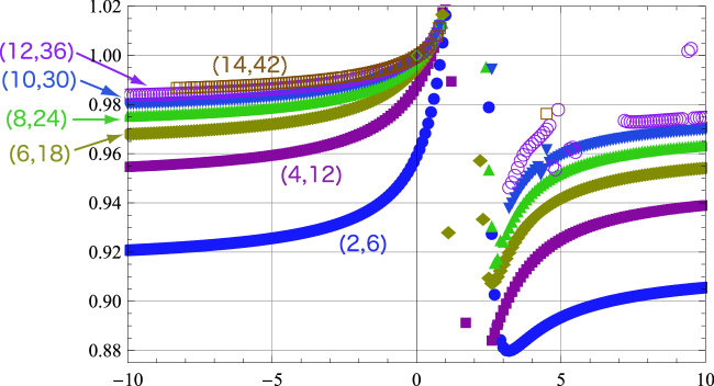
Figure 1: Plots of the action for various $a$-gauge solutions $\Psi_{a,L}$ in the $(L,3L)$ truncation. The horizontal axis denotes the value of $a$ and the vertical one denotes the normalized action $2\pi^{2}g^{2}S(\Psi_{a,L})/V_{26}$. The label $(L,3L)$ for each “curve” denotes the truncation level.

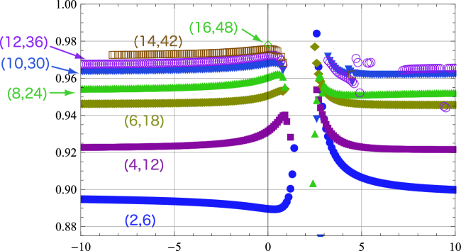
Figure 2: Plots of the gauge invariant overlap for various $a$-gauge solutions $\Psi_{a,L}$ in the $(L,3L)$ truncation. The horizontal axis denotes the value of $a$ and the vertical one denotes the normalized gauge invariant overlap $2\pi{\cal O}_{V}(\Psi_{a,L})/V_{26}$.

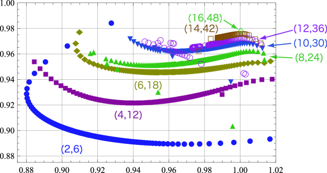
Figure 3: Plots of gauge invariants for various $a$-gauge solutions $\Psi_{a,L}$ in the $(L,3L)$ truncation. The horizontal axis denotes the normalized action and the vertical one denotes the normalized gauge invariant overlap. Each point denotes the value of $(2\pi^{2}g^{2}S(\Psi_{a,L})/V_{26},2\pi{\cal O}_{V}(\Psi_{a,L})/V_{26})$ for various $a$ values including $a=\infty$. The left part of the “curve” for each level corresponds to $4\lesssim a<+\infty$ and the right part corresponds to $-\infty<a\lesssim 1/2$. The plots for $a\to+\infty$ and $a\to-\infty$ are continuously connected at that of the Landau gauge ($a=\infty$).

For various $a$ in the region $a\lesssim 0$, $a\gg 1$, the normalized gauge invariants, action (Fig. 1) and gauge invariant overlap (Fig. 2), approach the value of one with increasing level. The speed of approach to one for the gauge invariant overlap is slower than that of the action as in the case of the Siegel gauge (Tables 1, 2). Although only $a=1$ gauge is ill-defined at the free level, interactions are included in the numerical calculations and hence the values in the region near $a\sim 1$ are unstable. In fact, the iterations do not converge in the dangerous region near $a\sim 1$.

Fig. 3 shows that both (normalized) gauge invariants for numerical solutions in the various $a$-gauges tend to converge to one with increasing truncation level. Namely, in the limit $L\to\infty$,

$$S(\Psi_{a,L})\to S(\Psi_{\rm Sch}),~{}~{}~{}~{}~{}~{}{\cal O}_{V}(\Psi_{a,L})\to{\cal O}_{V}(\Psi_{\rm Sch}),$$ (16)

are suggested for various $a$ ($-\infty\leqq a\lesssim 0$, $1\ll a\leqq\infty$). This seems to imply that not only the Siegel gauge ($a=0$) solution but also various $a$-gauge solutions constructed as in § 4 are all gauge equivalent to the Schnabl’s analytic solution.

6 Conclusion

We have evaluated gauge invariants (action and gauge invariant overlap) for numerical solutions in the $a$-gauge by level truncation. We have used an iterative method to construct these solutions and have checked consistency of the equation of motion for them. Except for the region at approximately $a=1$, where $a$-gauge condition becomes ill-defined at the free level, our various solutions in the $a$-gauge reproduce analytic values of Schnabl’s solution for tachyon condensation. The results are consistent with the expectation that various solutions in the $a$-gauge, including the Siegel gauge solution ($a=0$), are gauge equivalent to Schnabl’s solution. Therefore, they may represent a unique non-perturbative vacuum, where a D25-brane vanishes.

Acknowledgements

This work was supported in part by JSPS Grant-in-Aid for Scientific Research (C) (#21540269). The work of I. K. was supported in part by a Special Postdoctoral Researchers Program at RIKEN. The work of T. T. was supported in part by Nara Women’s University Intramural Grant for Project Research. Numerical computations in this work were partly carried out on the Computer Facility of the Yukawa Institute for Theoretical Physics in Kyoto University and the RIKEN Integrated Cluster of Clusters (RICC) facility.

References

- [1] M. Schnabl, Adv. Theor. Math. Phys. 10, 433 (2006) [arXiv:hep-th/0511286].
- [2] I. Ellwood, JHEP 0808, 063 (2008) [arXiv:0804.1131 [hep-th]].
- [3] T. Kawano, I. Kishimoto and T. Takahashi, Nucl. Phys. B 803, 135 (2008) [arXiv:0804.1541 [hep-th]].
- [4] T. Kawano, I. Kishimoto and T. Takahashi, Phys. Lett. B 669, 357 (2008) [arXiv:0804.4414 [hep-th]].
- [5] A. Sen and B. Zwiebach, JHEP 0003, 002 (2000) [arXiv:hep-th/9912249].
- [6] N. Moeller and W. Taylor, Nucl. Phys. B 583, 105 (2000) [arXiv:hep-th/0002237].
- [7] D. Gaiotto and L. Rastelli, JHEP 0308, 048 (2003) [arXiv:hep-th/0211012].
- [8] M. Asano and M. Kato, Prog. Theor. Phys. 117, 569 (2007) [arXiv:hep-th/0611189].
- [9] M. Asano and M. Kato, JHEP 0701, 028 (2007) [arXiv:hep-th/0611190].
- [10] I. Kishimoto and T. Takahashi, Prog. Theor. Phys. 121, 695 (2009) [arXiv:0902.0445 [hep-th]].
- [11] J. A. Shapiro and C. B. Thorn, Phys. Lett. B 194, 43 (1987).
- [12] M. Asano and M. Kato, Nucl. Phys. B 807, 348 (2009) [arXiv:0807.5010 [hep-th]].
- [13] H. Hata and S. Shinohara, JHEP 0009, 035 (2000) [arXiv:hep-th/0009105].