Today’s date:

Entanglement entropy and the complex plane of replicas

Ferdinando Gliozzi³ and Luca Tagliacozzo¹

³Dip. di Fisica Teorica and INFN, Università di Torino,

Via P. Giuria 1, 10125 Torino, Italy

¹School of Physical Sciences, the University of Queensland, QLD 4072, Australia

The entanglement entropy of a subsystem $A$ of a quantum system is expressed, in the replica method, through analytic continuation with respect to $n$ of the trace of the ${\rm n}^{th}$ power of the reduced density matrix ${\rm tr}\,\rho_{A}^{n}$. We study the analytic properties of this quantity as a function of $n$ in some quantum critical Ising-like models in 1+1 and 2+1 dimensions. Although we find no true singularities for $n>0$, there is a threshold value of $n$ close to 2 which separates two very different ‘phases’. The region with larger $n$ is characterised by rapidly convergent Taylor expansions and is very smooth. The region with smaller $n$ has a very rich and varied structure in the complex $n$ plane and is characterised by Taylor coefficients which instead of being monotone decreasing, have a maximum growing with the size of the subsystem. Finite truncations of the Taylor expansion in this region lead to increasingly poor approximations of ${\rm tr}\,\,\rho_{A}^{n}$. The computation of the entanglement entropy from the knowledge of ${\rm tr}\,\rho^{n}_{A}$ for positive integer $n$ becomes extremely difficult particularly in spatial dimensions larger than one, where one cannot use conformal field theory as a guidance in the extrapolations to $n=1$.

1 Introduction

The entanglement entropy has become a privileged measure of bipartite entanglement for pure states, that is of the entanglement between a subregion of the system and the rest of it. In order to compute it, one divides the system in the state $|\Psi\rangle$, into two complementary subsystems $A$ and $B$. The reduced density matrix of the region $A$ is obtained by tracing out the degrees of freedom inside the region $B$, $\rho_{A}={\rm tr}\,_{B}|\Psi\rangle\langle\Psi|$. The correlations between $A$ and $B$ give rise to a mixed state for $\rho_{A}$ whose von Neumann entropy $S_{A}\equiv-{\rm tr}\,\rho_{A}\log\rho_{A}$ is the entanglement entropy of the region $A$ (see e.g. [1] for reviews). Other quantities such as the Rényi ($R(\alpha)$) [2] and the Tsallis entropies ($T(\alpha)$) [3]

$$R(\alpha)=\frac{\log{\rm tr}\,\rho_{A}^{\alpha}}{1-\alpha}~{};~{}~{}~{}~{}T(\alpha)=\frac{{\rm tr}\,\rho^{\alpha}-1}{1-\alpha}~{},~{}~{}~{}\alpha>0~{},$$ (1.1)

are strictly related to the entanglement entropy of the block $A$. Indeed both of them coincide with it in the limit $\alpha\to 1$.

Studying directly the entanglement entropy in the ground state $|\Psi\rangle$ of a chosen Hamiltonian requires the ability to obtain such ground state. The complexity of this, in general, grows exponentially with the size of the system (recently new methods have been proposed to approximate the ground state of two dimensional systems that only scale polynomially with the system size [4, 5]).

However, when $\alpha$ in Eq. (1.1) is a positive integer $n$, the Tsallis and Rényi entropies can be computed in the context of quantum field theory (QFT), without the explicit knowledge of the ground state. The procedure is known as the “replica method” [6, 7] and is based on the fact that the expression $tr\rho_{A}^{n}$ can be written as a partition function of the model on a $n-$sheeted Riemann surface (or its generalization in $d+1$ dimensions), divided by $Z^{n}$, where $Z$ is the partition function of the original system . The entanglement entropy is obtained from it through an analytical continuation from positive integer $n$ to real $\alpha$ using $S_{A}=-\lim_{\alpha\to 1}\frac{\partial}{\partial\alpha}{\rm tr}\,\rho_{A}^{\alpha}$. Even if all values of ${\rm tr}\,\rho^{n}_{A}$ were provided for $n\in{\mathbb{N}}$, analytic continuation to real $\alpha$ might not be uniquely determined, as examples on disordered systems show [9]. It is therefore desirable to have some information on the analytical properties of ${\rm tr}\,\rho^{\alpha}_{A}$.

In the case of $1+1$ conformal field theories (CFT) the behaviour of the $T(n)$ when $A$ is composed by a single interval of length $\ell$ and is a part of an infinite gapless system is known to be [6, 7]

$${\rm tr}\,\rho_{\ell}^{n}=r_{n}\,\left(\frac{a}{\ell}\right)^{c(n-1/n)/6}~{}~{}.$$ (1.2)

Here $a$ is an ultraviolet (UV) cutoff, $c$ is the central charge of the associated CFT and $r_{n}$ is a non-universal function of $n$ which is known only in some special cases. In some cases even the full analytic continuation has been performed [8] allowing one to extract also the non universal additive corrections to the scaling of the entanglement entropy .

In $d>1$, however, CFT results are not available and one thus needs to carefully study the analytical properties of ${\rm tr}\,\rho^{\alpha}_{A}$ before trying to perform any analytic continuations of it.

The purpose of this work is to perform such a study by exploring the analytic properties of ${\rm tr}\,\rho_{A}^{\alpha}$ as a function of $\alpha$ in the whole complex plane for a class of quantum Ising-like critical models in both 1+1 and 2+1 dimensions. By doing this we uncover a highly non-trivial analytical behaviour of ${\rm tr}\,\rho_{A}^{\alpha}$ for $\alpha$ real in the interval $0<\alpha<2$. In all the models considered, we find a threshold value $n_{c}$ in the interval $1<n_{c}<2$ which divides ${\rm tr}\,\rho^{\alpha}_{A}$ into two ‘phases’. In the region with $\alpha\geq n_{c}$ the quantity ${\rm tr}\,\rho_{A}^{\alpha}$ behaves very smoothly as a function of $\alpha$; by expanding it in a Taylor series centred around any of the $\alpha_{o}>n_{c}$, we extract alternating series with monotone decreasing coefficients, then, any truncation $\sum_{k=0}^{n-1}c_{k}(\alpha-\alpha_{o})^{k}$ can be used to approximate ${\rm tr}\,\rho_{A}^{\alpha}$, the error of this approximation being less than $|c_{n}(\alpha-\alpha_{o})^{n}|$. For this reason we call the region $\alpha\geq n_{c}$ ‘perturbative’ region.

On the contrary, in the other ‘phase’, the Taylor expansions of ${\rm tr}\,\rho_{A}^{\alpha}$ with $0\leq\alpha_{o}<n_{c}$ has coefficients whose moduli are no longer monotone decreasing. They show a characteristic peak whose height increases with the size of $A$ (see for instance Fig.1). In this regime any truncation of the Taylor series becomes an increasingly poor approximation of $tr\,\rho_{A}^{n}$ as the size of $A$ grows. Thus we name the region $0\leq\alpha<n_{c}$ ‘non-perturbative’ region.

We shall see that the threshold value $n_{c}$ coincides with the point where the expression $\frac{{\rm d}^{2}{\rm tr}\,\rho_{A}^{\alpha}}{{\rm d}\alpha^{2}}+\frac{1}{3}\frac{{\rm d}^{3}{\rm tr}\,\rho_{A}^{\alpha}}{{\rm d}\alpha^{3}}$ changes sign, that is

$$\left(\frac{{\rm d}^{2}}{{\rm d}\alpha^{2}}+\frac{1}{3}\frac{{\rm d}^{3}}{{\rm d}\alpha^{3}}\right){\rm tr}\,\rho_{A}^{\alpha}|_{\alpha=n_{c}}=0~{}.$$ (1.3)

In the models we have considered it turns out that the two different ‘phases’ are separated by a smooth cross-over in both $d=1$ and $d=2$. However we cannot exclude that, in higher dimensions, this cross-over turns into a real phase transition. In fact it has been recently observed in Ref. [10] that the Rényi entropies in the $O(N)$ model undergo a phase transition as a function of $\alpha$ for $d$ close to 3. This happens in the same range of $\alpha$ in which the models we analyse develop the cross-over between the perturbative and the non-perturbative regions.

The above scenario has important consequences when trying to extract the entanglement entropy using the replica trick. On one side the absence of a real phase transition makes the analytic continuation (it involves) possible. On the other side, the different behaviour of the two ’phases’ implies that finding it can be really a non trivial task.

In fact, it is easy to find a simple function $f(n)$ which accurately reproduces ${\rm tr}\,\rho_{A}^{n}$ for integer $n$. However, if we make the ‘obvious’ extension to real $n$, by assuming that this functional form is also valid for real $n$, we obtain an incorrect value of the entanglement entropy.

By exemplifying this we also have the opportunity to compare two different methods. One is based on a recent algorithm proposed in Ref. [13] which allows us to accurately evaluate the reduced density matrix of a two-dimensional quantum system defined on a lattice of small size (in this paper we generally refer to this method as the Hamiltonian approach). The other one is based on the replica method and applies a simple technique described in Ref. [14] to directly measure ${\rm tr}\,\rho_{A}^{n}$ as the vacuum expectation value of a suitable observable in a Monte Carlo simulation, in any Euclidean lattice field theory.

The two methods agree on the Tsallis entropies $T(n)$ for a wide range of integer $n\geq 2$, once the UV cutoff of the two approaches are matched through a suitable conversion factor (this by itself is a non trivial result that provides a strong confirmation of the validity of both approaches). However there is a mismatch in the results for the entanglement entropy. Its value directly computed in the Hamiltonian approach (the correct one) is different from the one obtained in the Monte Carlo approach from the naive continuation of the behaviour of the Tsallis entropies for integer $n$ to real $\alpha$. This is a consequence of the intricate landscape of ${\rm tr}\,\rho_{A}^{n}$ close to $n=1$. The scenario we have outlined is common to all critical quantum systems in one and two dimensions we have analysed.

The contents of this paper are organised in several sections. In section 2 we describe the quantum models we want to study with different numerical methods and, where available, analytical results. In section 3 we describe both the Monte Carlo and the variational techniques we use to analyse quantum systems in 2+1 dimensions. Section 4 and 5 present the main results of this paper. In Section 4 we outline the presence of two ‘phases’ for ${\rm tr}\,\rho_{A}^{\alpha}$ by considering the features of its Taylor expansions. In section 5 we look for the Lee-Yang zeros and other possible singularities in the complex plane of $\alpha$ and we find no singularity related to the transition between these two regions. We unveil the presence of a smooth cross-over between the two regions. In Section 6 we discuss the effects of this scenario on entanglement entropy calculations. There we also present the comparison between the numerical results obtained with Monte Carlo and variational techniques. We conclude with a discussion of the results in Section 7.

2 The models

We analyzed the reduced density matrix ${\rm tr}\,\rho^{n}_{A}$ of the ground state near and at the quantum critical point in a series of one-dimensional spin $\frac{1}{2}$ chain systems and their two-dimensional generalizations. In particular, we considered the XY Hamiltonian

$$H_{\rm XY}=-\sum_{\langle i,j\rangle}\left[(1+\gamma)\sigma_{i}^{x}\sigma_{j}^{x}+(1-\gamma)\sigma_{i}^{y}\sigma_{j}^{y}\right]-2\,h\sum_{i}\sigma_{i}^{z}~{},$$ (2.1)

where $\langle i,j\rangle$ denote first neighbor sites, $\sigma_{i}^{\alpha}$ are Pauli matrices and $0\leq\gamma\leq 1$, $h\geq 0$. The subsystem $A$ is a block of neighboring nodes.

We applied mainly the numerical methods described in [11, 13], but we used also analytical results. Analytical calculations exist for the critical XX chain $(\gamma=0)$ [16], for the non-critical XY chain in a field [17] as well as for the Heisenberg chain [18].

Simplifications arise when mapping the quantum chains into classical two-dimensional classical spin systems [19]. The quantum XY chain can be mapped, at least for a part of the parameter range, into a classical Ising model on a triangular lattice [20]. In this way simple formulas can be easily obtained. For instance, if the subsystem $A$ is a block of spins of size $L$ much larger than the correlation length $\xi$, embedded into an infinite chain with periodic boundary conditions at zero temperature in the ordered phase ((i.e. $h<1$) the reduced matrix is independent of $L$ and can be written in the simple form [21]

$${\rm tr}\,\rho^{\alpha}_{L}=2\left(\frac{\prod_{n=1}^{\infty}(1+q^{n\,\alpha})}{\prod_{n=1}^{\infty}(1+q^{n})^{\alpha}}\right)^{2}~{},\,q=\exp(-2\epsilon)~{},$$ (2.2)

where the parameter $\epsilon$ which sets the scale is a known function of $\gamma$ and $h$ [20, 21]. The factor of two in front of (2.2) arises from the asymptotic degeneracy of the ground state in the broken ${\mathbb{Z}}_{2}$ symmetry for $h<1$. The exponent of two in (2.2) reflects instead the fact that the segment $L$ in a chain with periodic boundary conditions has two points of contact, i.e. two interfaces with the rest of the system.

We are interested in the critical limit $\epsilon\to 0$ where the infinite products (2.2) become slowly convergent, therefore we rewrite (2.2) in a more suitable form using the identity

$$\prod_{n=1}^{\infty}(1+q^{n\,\alpha})=\frac{\eta(2\alpha\tau)}{\eta(\alpha\tau)}\exp(-i\pi\alpha\tau/12)~{},\,\tau=i\frac{\epsilon}{\pi}~{},$$ (2.3)

thus

$${\rm tr}\,\rho^{\alpha}_{L}=2\left(\frac{\eta(2\alpha\tau)\,\,\eta(\tau)^{\alpha}}{\eta(\alpha\tau)\,\,\eta(2\tau)^{\alpha}}\right)^{2}~{}.$$ (2.4)

we introduced the Dedekind $\eta$ function

$$\eta(\tau)=q^{\frac{1}{24}}\prod_{n=1}^{\infty}(1-q^{n})$$ (2.5)

because it has a simple behaviour under the modular transformation $\tau\to-1/\tau$, namely

$$\eta(\tau)=\frac{1}{\sqrt{-i\tau}}\eta(-\frac{1}{\tau})~{},$$ (2.6)

and this leads to rapidly converging products. Precisely we have

$${\rm tr}\,\rho^{\alpha}_{L}=\exp\left(\frac{\pi^{2}}{12\epsilon}(\frac{1}{\alpha}-\alpha)\right)\,2^{\alpha}\,\left(\frac{\prod_{n=1}^{\infty}\left(1+\exp(-\frac{\pi^{2}}{\epsilon}n)\right)^{\alpha}}{\prod_{n=1}^{\infty}\left(1+\exp(-\frac{\pi^{2}}{\epsilon}\frac{n}{\alpha})\right)}\right)^{2}~{}.$$ (2.7)

Since $\frac{\pi^{2}}{\epsilon}\simeq\log\xi$, the first exponential tells us, according to [6, 7], that the associated CFT in the critical limit is the free fermion model with central charge $c=\frac{1}{2}$ as expected, however the exact expression (2.7) allows to discuss the analytical structure of the reduced density matrix in the whole complex replica plane. This discussion is postponed to Section 5.

For the other critical models, to our knowledge there are no analytical results available for the reduced density matrices, and we have to rely on a set of different numerical techniques. For the generic one dimensional critical XY chains we use the expression of the reduced density matrices of an interval in terms of the free fermionic modes described in Ref. [11] (for more recent results see e. g. Ref. [12]) and numerically diagonalise it. In the case of finite chains at the critical point we use the one dimensional version of the variational technique described in Ref. [13] that employs a Tree Tensor Network as an Ansatz for the ground state of the system.

In two dimensions we analyse the Ising model in a transverse field and the XX model on finite tori with both the Monte Carlo technique described in Ref. [14] and the variational technique of Ref. [13] that uses again a Tree Tensor Network. In 2D the subsystem $A$ is one half of a torus bounded by two parallel straight lines.

3 Monte Carlo simulations and variational algorithms

In QFT the quantity ${\rm tr}\,\rho^{n}_{A}$ can be written as the vacuum expectation value of a suitable observable ${\mathbb{O}}$ defined on a larger system composed of $n$ decoupled copies of the original system.

The canonical partition function $Z={\rm tr}\,e^{-\beta H}$ of a $d-$dimensional quantum system at inverse temperature $\beta$ can be computed in a standard way by doing the Euclidean functional integral in a $d+1$-dimensional hyper-cubic lattice $\Lambda=\{\vec{x},\tau\}$ $(x_{i},\tau\in{\mathbb{Z}})$ over fields $\phi(x)\equiv\phi(\vec{x},\tau)$ periodic under $\tau\to\tau+\beta$. Therefore the system composed of $n$ independent replicas of the original system is described by the $n-$th power of $Z$:

$$Z^{n}=\int\prod_{k=1}^{n}{\cal D}[\phi_{k}]e^{-\sum_{k=1}^{n}S[\phi_{k}]}~{},$$ (3.1)

where $\phi_{k}$ is a field configuration associated to the $k-$th copy and $S[\phi]$ is the Euclidean action.

In the replica approach to entanglement the subsystem $A$ establishes a process of transferring information among the $n$ replicas through a specific coupling: the lattice links coming out of nodes of $A$ and directed into the (Euclidean) time direction $\tau$ cyclically connect the copy $k$ with the copy $k+1$ [6, 7]. Let us denote with $S_{A}[\phi_{1},\phi_{2},\dots,\phi_{n}]$ the corresponding coupled action. It is easy to see that the quantity

$${\mathbb{O}}=e^{-\left(S_{A}^{(n)}[\phi_{1},\phi_{2},\dots,\phi_{n}]-\sum_{k=1}^{n}S[\phi_{k}]\right)}~{},$$ (3.2)

has the desired property. In fact its vacuum expectation value in the system of $n$ independent copies of the original system is

$$\langle{\mathbb{O}}\rangle_{n}=\frac{\int\prod_{k=1}^{n}{\cal D}\phi_{k}\,{\mathbb{O}}\,e^{-S[\phi_{k}]}}{Z^{n}}=\frac{\int\prod_{k=1}^{n}{\cal D}\phi_{k}\,e^{-S_{A}^{(n)}}}{Z^{n}}=\frac{Z_{n}(A)}{Z^{n}}={\rm tr}\,\rho_{A}^{n}~{}.$$ (3.3)

$Z_{n}(A)$ is the partition function of the system in the $n$ coupled replicas.

This method can be simply implemented in Monte Carlo simulations. Here we apply it to the case in which the system is a periodic lattices of size $L^{2}\times 8L$, where the longer direction is the Euclidean time. We verified that the Euclidean time is large enough to ensure the absence of measurable finite temperature effects. The Monte Carlo simulations were performed with a particularly efficient implementation for the Ising and $q-$ state Potts model described in [14] and with the standard action of the isotropic Ising model on a cubic lattice

$$S=-\sum_{\langle i,j\rangle}S_{i}\,S_{j}~{};~{}~{}S_{i}=\pm 1~{}.$$ (3.4)

All simulations were made at the critical coupling $\beta\simeq 0.221652$.

With this method we compute directly the Tsallis entropies for integer $n$. A discussion of the results we obtained is postponed to Section 6.

Using the techniques of Ref. [13] we also extract an accurate variational approximation to the ground state with a Tree Tensor Network of the corresponding quantum model. This is the quantum Ising model on a square torus at its critical point obtained by setting the parameters of the Hamiltonian in Eq. 2.1 to $\gamma$=0 and $2h=3.044$ [15]. This approach is limited by the exponential growth of the Hilbert space with the system size. The benchmark calculations presented in Ref. [13] show that, nevertheless, it can be used safely at least for tori of dimension up to $10\times 10$. It has the strong advantage that it allows us to extract the complete spectrum of the reduced density matrix $\rho_{A}$ for arbitrary blocks. It thus provides a way to directly compute ${\rm tr}\,\rho^{\alpha}$ for an arbitrary complex $\alpha$ and also to directly compute the entanglement entropy. A detailed explanation on how to compute the reduced density matrices in this approach is contained in Ref. [13]. We also postpone the discussion of the numerical results for both the Tsallis and entanglement entropy extracted with this method to Section 6.

4 The two regions of Tsallis entropies

As we discussed in the introduction the Taylor expansions of ${\rm tr}\,\rho_{A}^{\alpha}$ can be used to study the behaviour of the Tsallis and Rényi entropies as a function of $\alpha$ and identify two very different regions. In order to exemplify this idea we have to express the Taylor expansion of ${\rm tr}\,\rho_{A}^{\alpha}$ about $\alpha=1$ in a convenient form. Let $p_{i}$ be the non vanishing eigenvalues of $\rho_{A}$. At first the normalisation of $\rho_{A}$ implies

$${\rm tr}\,\rho_{A}=\sum_{i}p_{i}=1~{}.$$ (4.1)

Through the chain of identities

$${\rm tr}\,\rho_{A}^{\alpha}=\sum_{i}p_{i}p_{i}^{\alpha-1}=\sum_{i}p_{i}\sum_{k=0}^{\infty}(\log\,p_{i})^{k}\frac{(\alpha-1)^{k}}{k!}=\sum_{k=0}^{\infty}\frac{\langle\,(\log\,p)^{k}\rangle}{k!}(\alpha-1)^{k}$$

$$=\sum_{k=0}^{\infty}\frac{{\rm tr}\,\rho_{A}(\log\rho_{A})^{k}}{k!}\,(\alpha-1)^{k}\equiv\sum_{k=0}^{\infty}c_{k}\,(\alpha-1)^{k}~{},$$ (4.2)

we define the Taylor coefficient $c_{k}=\frac{{\rm tr}\,\rho_{A}(\log\rho_{A})^{k}}{k!}$. Since the eigenvalues of ${\rm tr}\,\rho_{A}$ are smaller than 1 the Taylor expansion is an alternating series, i.e. $c_{k+1}=-c_{k}$. This is an important feature when discussing the possible location of the singularities in the complex $\alpha$ plane or in estimating the error we make in truncations of the Taylor expansions, as we shall see later. From the spectrum of $\rho_{A}$ we can explicitly compute the above Taylor expansion.

As an example, the method described in Ref. [11] can be used to compute the reduced density matrix of a block of spins of an infinite critical Ising chain. From it, we compute the moduli of the first Taylor coefficients of ${\rm tr}\,\rho_{A}^{\alpha}$ and plot them in Fig.1 (a) for four different values of $L$. It is interesting to notice that the plot shows a peak at some value of $k>1$ and that its height increases with $L$.

Figure 1: Plot of the moduli of the coefficients of the Taylor expansion of of ${\rm tr}\,\rho_{A}^{\alpha}$ about $\alpha=1$ for (a) the 1D Ising model in transverse field at the critical point and (b) the 2D Ising model defined on a torus of $L\times L$. In (a) the block $A$ consists of $L$ adjacent spins of the infinite chain with $L=64,128,256,512$. The spectrum of the reduced matrix $\rho_{A}$ is obtained applying the method described in Ref.[11]. In (b) the subsystem $A$ is half a torus $L\times L$ with $L=4,6,8,10$. The spectrum is obtained by using the method described in Ref. [13]. In both dimensions the height of the peaks of the Taylor coefficients increases with L.

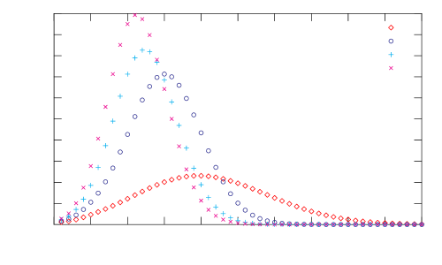
A similar behaviour can be observed in a quantum two-dimensional critical Ising model on a torus $L\times L$ as shown in Fig.1 (b). There we plot again the absolute value of the Taylor coefficients of the expansion of ${\rm tr}\,\rho_{A}^{\alpha}$ about $\alpha=1$ for four different values of $L$. The subsystem $A$ in this case is half a torus. The reduced density matrices $\rho_{A}$ are obtained with the techniques described in Ref. [13]. By comparing the same expansion for different systems sizes, $L=4,6,8,10$ we appreciate how the peaks move with $L$ and, more importantly, their height increases with $L$.

By varying the expansion centre of the Taylor expansions $\alpha_{o}$ we can check the behaviour of the coefficients in other regions of the $\alpha$ axis. The expression for the coefficients of the Taylor expansion about $\alpha=\alpha_{o}$ is

$$c_{k}[\alpha_{o}]=\frac{{\rm tr}\,\rho_{A}^{\alpha_{o}}(\log\rho_{A})^{k}}{k!}~{}.$$ (4.3)

We repeat the same study presented in Fig. 1 in the region $1\leq\alpha_{o}\leq 2$ and observe that the peaks of Fig. 1 (a) and (b) start moving to left as we increase the value of $\alpha_{o}$ to eventually disappear at a threshold value $\alpha_{o}=n_{c}\leq 2$. In the region where the peaks are present we cannot obtain a good approximation of ${\rm tr}\,\rho_{A}^{\alpha}$ by truncating the power series (4.2) down to only few terms. Also, the convergence of the series (4.2) deteriorates with the size of the system, preventing the possibility to find a good truncation scheme independent of the system’s size. For this reason we call the region $\alpha<n_{c}$ the non-perturbative region .

For $\alpha_{o}>n_{c}$ the coefficients $c_{k}[\alpha_{o}]$ become monotone decreasing in modulus. As a consequence, in this region, the partial sum $s_{k_{o}}=\sum_{k=0}^{k_{o}}c_{k}[\alpha_{o}](\alpha-\alpha_{o})^{k}$ can be used to approximate ${\rm tr}\,\rho_{A}^{\alpha}$ with an error smaller than $c_{k_{o}+1}[\alpha_{o}](\alpha-\alpha_{o})^{k_{o}+1}$. In this case thus, we call the region $\alpha>n_{c}$ the perturbative region.

(a) (b)

Figure 2: (a) Scaling behaviour of the threshold $n_{c}$ that separates the perturbative from the non-perturbative region, as a function of the size $L$ of the block. (a) 1D quantum critical Ising chain. The rhombi refer to blocks embedded into an infinite chain, while the circles refer to half of a finite chains of length $2L$. The threshold values located respectively at $n_{i}=1.414(5)$ and $n_{h}=1.391(1)$ are approached in both cases with a power law with the same exponent $1/8$ . Data for the infinite chain are obtained using the method of Ref. [11] while for finite chains with the one dimensional version of the method of Ref. [13]. (b) 2D quantum critical Ising models on several tori. The blocks are half tori. Here also the location of $n_{c}$ approaches its thermodynamic limit as a power law with exponent $1/2$ and the limit is located at $n_{t}=1.835(1)$. The data are obtained with the technique introduced in Ref. [13].

The threshold value $n_{c}$ is defined as the minimal value of $\alpha$ such that

$$|c_{k+1}[\alpha]|\leq\,|c_{k}[\alpha]|~{},~{}~{}k=0,1,\dots~{}.$$ (4.4)

that is, the Taylor coefficient $c_{k}$ are monotonically decreasing functions of $k$. In all the models we have considered, as soon as the criterion in Eq. 4.4 is fulfilled by the second and third coefficients, that is, $|\,c_{3}[\alpha]|\leq|\,c_{2}[\alpha]|$, it is also fulfilled by all the others pairs. Using this property we can define $n_{c}$ as the solution of Eq.(1.3) anticipated in the introduction. We can also use

$$s={\rm Sign}\left(\frac{{\rm d}^{2}{\rm tr}\,\rho_{A}^{\alpha}}{{\rm d}\alpha^{2}}+\frac{1}{3}\frac{{\rm d}^{3}{\rm tr}\,\rho_{A}^{\alpha}}{{\rm d}\alpha^{3}}\right)~{},$$ (4.5)

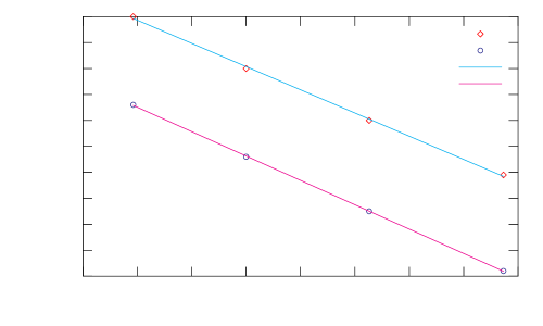
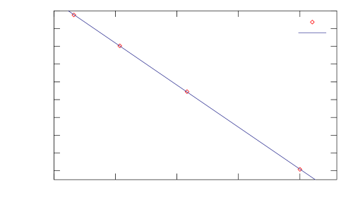
the sign of the expression (1.3) defining $n_{c}$, as a sort of order parameter distinguishing between the perturbative $(s>0)$ and non-perturbative $(s<0)$ ‘phases’. As expected, the value of the threshold depends on the size of the system, i.e. $n_{c}=n_{c}(L)$. By analysing this dependence we found that in our critical systems $n_{c}(L)$ obeys a simple power law

$$n_{c}(L)=n_{o}+b/L^{\epsilon}~{},$$ (4.6)

where $\epsilon=\frac{1}{8}$ in the 1D critical Ising model and $\epsilon=\frac{1}{2}$ in the 2D critical Ising model. It is also interesting to notice that $n_{o}\leq 2$ for all the models we have analysed (see Figs. 2 (a) and (b)).

5 The nature of the transition

Having uncovered the presence of two different regions for Tsallis (and Rényi) entropies as functions of $\alpha$, we now want to investigate whether these two regions are well separated phases divided by a transition point or if instead they are different regions of the same phase smoothly connected through a cross-over. Of course, these two scenarios have very different physical implications. In the case where the two regions are separated by a true phase transition for some real $n_{c}$ in the range $1<n_{c}<2$, there would be no possibility to analytically continue the Tsallis entropy from one phase to the other. This, for example, would imply that the entanglement entropy could not be obtained via the replica method. This is unlikely to happen in one dimensional critical systems since the entanglement entropy has been already successfully computed with the replica trick in some 1+1 CFT [8]. In two dimensions however, for the models we are considering, the entanglement entropy has not yet been obtained analytically and one can be concerned about if with the replica trick is a viable method to perform such a calculation.

In order to settle the nature of the transition between the perturbative and non perturbative regions we start by considering the radius of convergence of the Taylor expansion of ${\rm tr}\,\rho_{A}^{\alpha}$ around $\alpha_{o}=1$. It indeed measures the distance between the centre of the Taylor expansion and the nearest singularity in the complex $\alpha$ plane. As the expansions of ${\rm tr}\,\rho_{A}^{\alpha}$ is an alternating series its possible singularity belongs to the real axis at the left side of the expansion centre. We can also argue on general grounds that the singularity should be at $\alpha$ greater or equal to zero.

Indeed we expect at least a singularity of ${\rm tr}\,\rho_{A}^{\alpha}$ at $\alpha=0$, since ${\rm tr}\,\rho_{A}^{0}$ measures the number of degrees of freedom of the subsystem $A$. This number diverges exponentially with its size (Eq.(1.2), for example, presents an essential singularity at $\alpha=0$).

For the sake of completeness one should remember that, when the system is in a product state (situation that does not arise close to a critical point) there is no singularity at $\alpha=0$, even in the thermodynamic limit. This happens, i.e., in the XY model described in (2.1) as one approaches the disorder line $h^{2}+\gamma^{2}=1$ in the ordered phase $(h\leq 1)$ . There the ground state becomes the superposition of two product states [24] and ${\rm tr}\,\rho^{\alpha}=2^{1-\alpha}$. Similarly, there is a class of $z=2$ quantum critical points in two spatial dimensions where a very simple form for ${\rm tr}\,\rho^{\alpha}_{A}$ has been proposed [25], namely ${\rm tr}\,\rho^{\alpha}_{A}=(Z_{D}/Z_{F})^{\alpha-1}$, where $Z_{D}$ and $Z_{F}$ are the partition functions of the associated system with suitable boundary conditions which select the subsystem $A$.

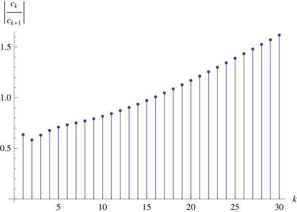
In the cases of highly entangled states we consider here, however, we do expect a singularity at $\alpha=0$ in the thermodynamic limit and therefore the radius of convergence of the expansion (4.2) of ${\rm tr}\,\rho_{A}^{\alpha}$ centred around $\alpha_{o}=1$ should not exceed 1. A precise value for it can be extracted using the ratio test. This states that if the limit $r=\lim_{k\to\infty}\left|\frac{c_{k}}{c_{k+1}}\right|$ exists, it coincides with the convergence radius $r$. In a finite system, there is no true singularity and the radius of convergence of the series is infinite. However we expect we are still able to identify what would turn into a true singularity in the thermodynamic limit, by studying the sequence $\left\{\left|\frac{c_{k}}{c_{k+1}}\right|\right\}$.

We anticipate that, notwithstanding there are clues to the presence of singularities in the thermodynamic limit, a careful analysis allows us to exclude it: the only possible singularities of ${\rm tr}\,\rho^{\alpha}$ lie on the imaginary axis of $\alpha$.

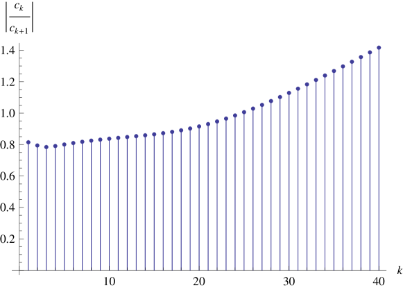
These ratio sequences show a sort of plateaux at a value $r$ in a certain range of $k$ before they eventually run away for $k>k_{o}$. The point $k_{o}$ moves to the right within the size of the system, revealing longer and longer plateaux. This has been observed in all the models we have analysed. For instance, we may compute the required ratios $\frac{c_{k}}{c_{k+1}}$ from the Taylor coefficients of a $L=512$ block of a critical one dimensional Ising model, by using the coefficients plotted in Fig. 1 (a). These ratios are plotted in Fig. 3.

(a)

(b)

Figure 3: (a) Ratio $\frac{c_{k}}{c_{k+1}}$ as a function of $k$ obtained from the Taylor coefficients of ${\rm tr}\,\rho_{A}^{\alpha}$ about $\alpha_{o}=1$ plotted in Fig. 1. The ratios oscillate for $k\leq 20$ around $0.8$ before they run away. This could be a hint of a finite radius of convergence for this Taylor series in the thermodynamic limit, generated by a conjectural singularity located somewhere around $1-0.8=0.2$. In (b) the ratio test shows a similar behaviour for the $d=2$ critical Ising model on a torus $L\times L$ with $L=6$.

There we can see that the ratios oscillate for a while around a value smaller than 1 before running away. This suggests that a new singularity on the right side of the one we already expect at $\alpha=0$ might exist in the thermodynamic limit.

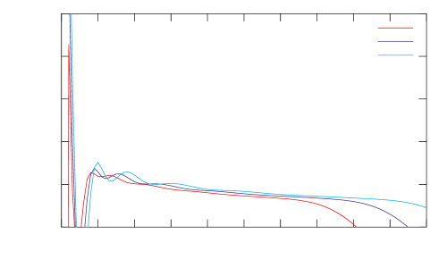
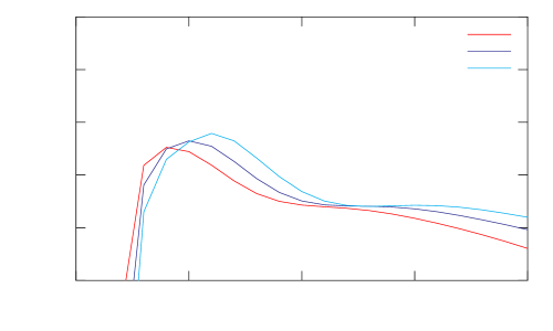
This scenario is further supported by studying the Taylor expansions around other positive values of $\alpha$. If there were a true singularity on the real axis, the function

$$A[\alpha,k]=\alpha-\left|\frac{c_{k}[\alpha]}{c_{k+1}[\alpha]}\right|~{},$$ (5.1)

would converge to the coordinate location of the singularity in the thermodynamic limit and would not dependent on the value of $\alpha$. In a finite system we expect that $A[\alpha,k]$ should approach to a constant value independent of $\alpha$ for a certain range of $k$, and this range should increase with the size of the system. This behaviour can be observed, for instance, in Fig. 4 (a) where we plot $A[\alpha,k]$ for the $L=512$ block of the critical quantum Ising chain (the same already considered in Fig. 1 (a)), and in Fig.4 (b) where we plot the same quantity for the two-dimensional Ising model on a torus of side $L=6$.

Still all the above signatures are not sufficient to conclude that there is a true singularity for real $\alpha$ in the thermodynamic limit in ${\rm tr}\,\rho^{\alpha}$.

Figure 4: Plot of the function $A[\alpha,k]$ defined in (5.1) for different values of $\alpha$. This quantity should converge in the thermodynamic limit to the location of the alleged singularity. The system in (a) is the same quantum Ising chain of Fig.1. The system in (b) is the critical Ising model on a torus $L\times L$ with $L=6$. Note that the position of the flexes on the $y$ axis is nearly independent of $\alpha$.

As shown by Eq. (3.3), ${\rm tr}\,\rho_{A}^{n}$ can be written as the ratio of two partition functions. This allows us to apply a Lee-Yang [26] analysis to it.

In discrete systems of finite size partition functions are analytic with respect to their parameters because they are finite summations of positive terms. For the same reason they do not have zeros on the real axis. However there can exist zeros on the complex plane of certain control parameter, $\alpha$ in our case, which are generally named Lee-Yang zeros [26]. In general, the Lee-Yang zeros are apart from the real axis as long as the system size $L$ is finite. However, if a phase transition occurs at a critical value $n_{o}\in{\mathbb{R}}$, the distribution of zeros becomes dense and accumulate on curves. The singularities of the free energy associated to this transition lie on the end points of these curves. As $L\to\infty$ these end points move towards the real axis, eventually touching it at the location of the critical point $n_{o}$.

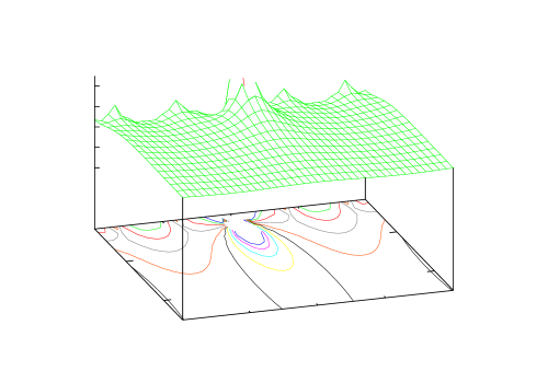
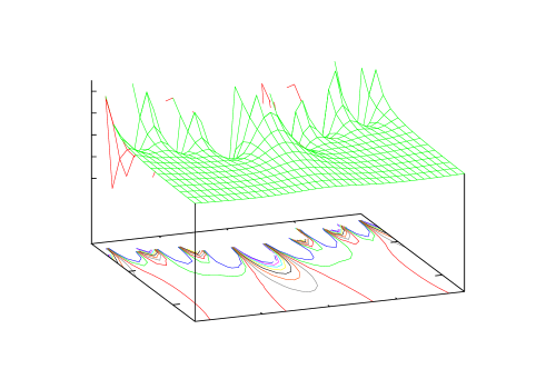
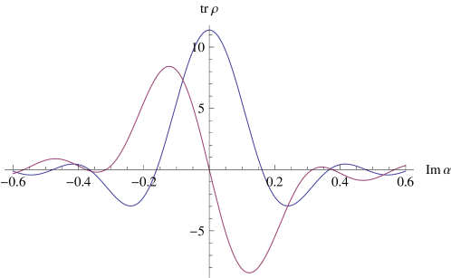
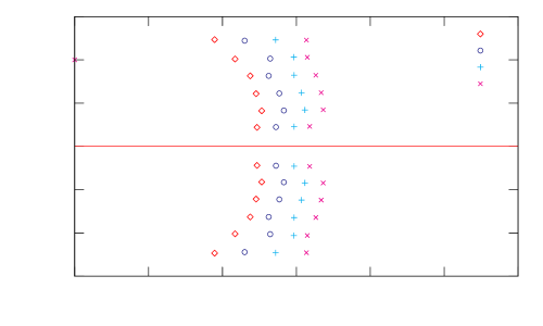
In the case of ${\rm tr}\,\rho_{A}^{n}=\frac{Z_{n}(A)}{Z^{n}}$ besides the surviving zeros of the numerator there could also be poles due to zeros of the denominator. As an example, the exact expression of the reduced density matrix in Eq. (2.7) for the non-critical XY chain, presents a singularity at $\alpha=0$ (the same as the singularity of (1.2)) but no zeros. It contains instead a huge number of double poles at $\alpha=\pm i\frac{n\,\pi}{(2k-1)\epsilon}$ for any pair of integers $k,n\in{\mathbb{N}}$. This set is dense on the imaginary $\alpha$ axis. The plot of $\Re e\,{\rm tr}\,\rho_{L}^{\alpha}$ is presented in Fig. 5 (a) and reflects this intricate structure. A similar landscape can be observed by considering the quantum two dimensional critical Ising model on a torus (see Fig. 5 (b)) where one can locate few zeros (see e. g. Figure 6) close to the region $\Re e\,\alpha=0.3$ where the ratio test give hints of a singularity.

The important outcome of this study is that in all the models we have analysed both in $d=1$ and in $d=2$, these Lee-Yang zeros, which are true singular points of the Rényi entropy (1.1) in the complex plane, do not become denser as the size of the system increases nor they approach the real axis (see Figure 7). In the thermodynamic limit then, the apparent singularity on the real axis identified by the ratio test of Taylor coefficients does not occur. The behaviour of flexes described by Eq.(5.1) is probably only a consequence of the presence of some structures in the complex $\alpha-$plane (zeros and/or peaks) which do not evolve into a true singularity in the thermodynamic limit.

The lesson we learn from this analysis is twofold. On the one hand there is no true phase transition between the two regions where the Tsallis entropies show very different behaviour. The transition is only a smooth cross-over. On the other hand the behaviour of ${\rm tr}\,\rho^{\alpha}$ shows an intricate landscape in the region $\Re e\,\alpha<n_{c}$ while it is very smooth in the complementary region $\Re e\,\alpha>n_{c}$. As a consequence a naive analytical continuation of the results obtained for the Tsallis entropies in the perturbative region is likely to fail to reproduce the correct entanglement entropy. We will provide an example of this fact in the following section.

(a)

(b)

Figure 5: Plot of $\Re e\,{\rm tr}\,\rho^{\alpha}_{L}$ for the non-critical XY chain in the complex replica plane (a) and in the 2D Ising model at at the critical point for half a $6\times 6$ torus (b). Both plots show a very rugged landscape with several dips and peaks.

Figure 6: Plot of the real and imaginary parts of ${\rm tr}\,\rho^{\alpha}$ along the imaginary axis $\Im\,m\,\alpha$ with $\Re e\,\alpha=0.3$ for the 2D Ising model on a $6\times 6$ torus at the critical point. The imaginary part is the curve intersecting the origin. The intersection of the two curves identifies a pair of zeros at $\Im\,m\,\alpha=\pm 0.3655$.

(a) (b)

Figure 7: Finite size scaling of the zeros of ${\rm tr}\,\rho^{\alpha}_{L}$ in the complex $\alpha$-plane. for (a) several blocks of different length in the one dimensional XY model and (b) several half tori of different size in the 2D quantum Ising model at the critical point. In both cases, the zeros do not approach the real axis nor their number grows with the size of the system. This fact demonstrates that they cannot originate a singularity for real $\alpha$ in thermodynamic limit.

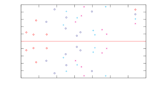
As an aside, it is interesting to observe the striking resemblance between the location and shape of the zeros distribution of Fig. 7 and those found in certain disordered systems [27]. In the latter case the replicas are coupled together no longer by the subsystem $A$, but by the quenched average, which restores the translational invariance of the system. As a consequence the latter system develops in thermodynamic limit a true singularity associated to replica symmetry breaking.

Figure 8: Fit of the Monte Carlo estimations of ${\rm tr}\,\rho_{L}^{n}$ (rhombi) to the function (6.1) in a 3D critical Ising model. The circles are the values calculated in the corresponding quantum system in 2+1 dimensions with the method of [13] with the length rescaled by a suitable conversion factor.

6 The entanglement entropy mismatch

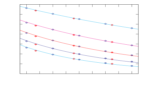
In order to test the consequences of the intricate structure of ${\rm tr}\,\rho^{\alpha}$ in the complex plane we have performed a numerical experiment. This consists in computing the entanglement entropy using the replica trick from the results obtained in a Monte Carlo simulation. For the 2D Ising model on a torus indeed there are still no analytical predictions on value of the parameter appearing in the proposed form of the scaling of the entanglement entropy. Some numerical results have been recently obtained in Ref. [13]. Here we have computed ${\rm tr}\,\rho_{A}^{n}$ for $n=2,3,4,5,6$ with the Monte Carlo technique described in Sect. 3 when $A$ is a half of the torus, the same geometry studied in Ref. [13]. The results we obtain agree with the ones computed from the data of Ref. [13] provided we introduce a suitable conversion factor between the lattice spacings of these two different regularisation schemes. A good agreement is indeed obtained by multiplying the lengths measured in the Hamiltonian approach by a conversion factor $f\simeq 1.45$ (see Fig.8). This agreement is a good check of the validity of both methods. To our knowledge it is also the first direct comparison between two different non-perturbative techniques on entanglement entropy, one involving quantum mechanical tensor network simulations and the other one using statistical mechanics Monte Carlo integration. This is what we expect from universality, indeed, these two methods deal with very different systems (in one case the model studied is the 3D classical Ising model while in the other case it is the 2D Quantum Ising model). They show the same behaviour close to the critical point because they belong to the same universality class.

We can now try to extract a function $f(L,n)$ from the data describing the behaviour of ${\rm tr}\,\rho^{n}$ in the whole range of $n$ and $L$ considered . The function should depend on only few parameters and is chosen in such a way to agree, in the $n\to 1$ limit, with the expected general form of the critical entanglement entropy in 2+1 dimensions [23, 10]. A sufficiently good fit (a reduced $\chi^{2}=1.75$ for 17 degrees of freedom) is given by the three-parameter function

$$f(n,L)=\exp[-a\,(n-\frac{1}{n^{3}})2\,L-(b+\frac{c}{2L})(n-\frac{1}{n})]$$ (6.1)

with

$$a=0.01177(92)\,,~{}b=0.0594(55)\,,~{}c=-0.378(73)~{}.$$ (6.2)

The ‘obvious’ extension to real $n$, is performed by assuming that this functional form should also be valid for real $n$. The entanglement entropy then is given by

$$S_{L}\equiv-{\rm tr}\,\rho_{A}\log\rho_{A}\,=^{\hskip-5.69046pt?}~{}-\lim_{n\to 1}\frac{{\rm d}}{{\rm d}n}f(n,L)=8\,a\,L+2b+c/L.$$ (6.3)

Due to our choice of the parametrisation (6.1) the entanglement entropy has the expected functional form $S_{L}=c_{1}\,2L+c_{0}+\frac{c_{-1}}{2L}.$ The numerical coefficients we extract however, apart from the ’area term’ $c_{1}$, do not coincide with the ones extracted from the direct study of the entanglement entropy computed in Ref. [13]. If we call the parameter extracted in Ref. [13] $S_{L}=c_{1}^{\prime}2L+c_{0}^{\prime}+\frac{c_{-1}^{\prime}}{2L}$, taking into account the conversion factor $f$, we would expect from the values reported in (6.2) that

$$c_{1}^{\prime}=c_{1}\,f=0.0682(5)~{},\,c_{0}^{\prime}=c_{0}=0.12(1)~{},\,c_{-1}^{\prime}=c_{-1}/f=-0.52(10).$$ (6.4)

On the other hand their direct numerical determination [13] provides different results

$$c_{1}^{\prime}=0.06722(18)~{},\,c_{0}^{\prime}=0.0250(21)~{},\,c_{-1}^{\prime}\simeq 0~{}.$$ (6.5)

Figure 9: Plot of the moduli of the coefficients of the Taylor expansion about $n=1$ of Eq.(1.2) with $r_{n}=1$. Although it fits perfecltly the behaviour of ${\rm tr}\,\rho^{n}_{L}$ of the same system of Fig. 1 (a) with $L=512$ in the range $n\geq 2$, its analytic continuation to $n\simeq 1$ region does not reproduce the true Taylor expansion plotted in Fig.1 (a).

We attribute the mismatch of the entanglement entropy to the the different behaviour of the the regions $\Re e\,\alpha<n_{c}$ and $\Re e\,\alpha>n_{c}$.

A further confirmation of this can be obtained by computing, in the Hamiltonian approach, ${\rm tr}\,\rho_{A}^{\alpha}$ for some real (or complex) $\alpha$ in the non-perturbative region. If we add to the fitted data some of these points the quality of the fit to (6.1) rapidly deteriorates.

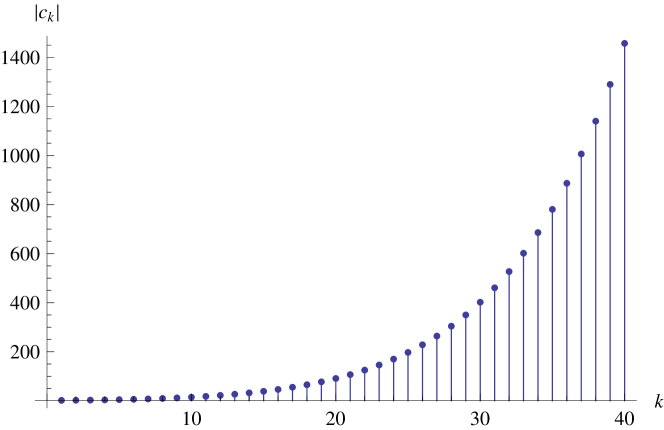
One can check that a similar phenomenon holds also for $d=1$ models. Indeed, considering again the critical XY system in which the subsystem $A$ is composed by a block of $L=512$ adjacent spins, ${\rm tr}\,\rho_{L}^{n}$ can be evaluated with the method of [11] and the data with $n\geq 2$ can accurately fitted with Eq.(1.2) ignoring the $n$ dependence of the non-universal coefficient $r_{n}$ which is known to be neglegible in such a range [22]. If now we assume that this functional form with $r_{n}=1$ is also valid for real $n$ and try to evaluate this quantity near $n=1$ we obtain incorrect results for the entanglement entropy. As an example the Taylor coefficients of this fitting function are plotted in Fig. 9 and should be compared with the same coefficients directly evaluated on ${\rm tr}\,\rho_{L}^{n}$ (see Fig.1 (a) ). They show a completely different shape. Again this mismatch has to be attributed to having applied to the fitting function (1.2) with $r_{n}=1$, which accurately describes the behaviour of ${\rm tr}\,\rho^{n}$ in the perturbative region (i.e. $n>n_{c}$), the ‘obvious’ extension to real $n$ close to $n=1$ which lies in the non-perturbative region.

7 Discussion

In this work we analysed the trace of the $n-$th power of the reduced density matrix ${\rm tr}\,\rho_{A}^{n}$ associated to a subsystem $A$ in some Ising-like quantum models in both one and two spatial dimensions near and at a quantum critical point at zero temperature. We unveiled that, depending on the value of $n$, ${\rm tr}\,\rho_{A}^{n}$ shows two very different behaviours. If $n$ is larger than a threshold value $n_{c}$ -located in the interval $1<n<2$- its behaviour is very smooth. In particular the alternating coefficients of its Taylor expansions, $c_{k}$ are monotone decreasing. In this regime the error involved in a truncation of the series does not exceed the first excluded term and can be always chosen to be very small. We label this region ‘perturbative’ region.

In the range $n<n_{c}$, on the other hand, the $|c_{k}|$’s are no longer monotone decreasing function of $k$ but they present a characteristic peak (see Fig.1 ) whose height increases with the size of the block considered. Any truncated Taylor expansion, in this region, provides an increasingly poor approximation of ${\rm tr}\,\rho_{A}^{n}$ as the size of $A$ increases. This is the region that we label ‘non-perturbative’.

The transition between these two regions turns out to be a smooth cross-over. The dependence of the threshold $n_{c}(L)$ on the size of the subsystem obeys a power law described in Eq. (4.6). We determined the critical exponents ruling this power law for the Ising model in both one and two dimensions. It would be interesting to investigate whether this cross-over is somehow related to the phase transition close to n=2 recently observed in [10] near $d=3$.

The above scenario has important consequences when considering the analytical continuation involved in the computation of the entanglement entropy with the replica trick. This continuation is possible in one and two dimensions, as there is no phase transition between the perturbative region (where both analytical results from QFT and numerical results from Monte Carlo algorithms are available) and the non-perturbative region (where the entanglement entropy is located). However its form is not the naive expression obtained by promoting the simple expression obtained in the perturbative region for integer $n$ to general $\alpha$, as we have explicitly shown in Section 6 .

From our analysis, the Rényi and Tsallis entropies seem to emerge as a privileged measures of entanglement in QFT. Although they lack the nice theoretical information properties of the entanglement entropy [28], their analytic properties as functions of the $\alpha$ parameter seem to contain some new information on the entanglement. This has been considered recently in the context of quantum criticality [29, 30, 10] and topological order [31].

LT acknowledges the financial support from the QuSim group of the University of Queensland, the stimulating discussions with P. Corboz and the enlightening comments on entanglement measures of Prof. G. Vidal.

References

- [1] L.Amico, R.Fazio, A. Osterloh and V. Vedral, Rev. Mod. Phys. 80, 517 (2008), arXiv quant-ph/0703044; J. Cardy, Eur. Phys. J. B 64 , 321 (2008), arXiv 0708.2978; J. Eisert, M. Cramer and M.B. Plenio, arXiv 0808.3773.
- [2] A. Rényi, “ Probability Teory”, North-Holland, Amsterdam,1970.
- [3] C. Tsallis, J. Stat. Phys.52 (1988) 479.
- [4] G. Evenbly, G. Vidal Phys. Rev. Lett. 102, 180406 (2009) arXiv:0811.0879.
- [5] F. Verstraete, J.I. Cirac, V. Murg Adv. Phys. 57,143 (2008) arXiv:0907.2796.
- [6] C. Holzhey, F. Larsen, F. Wilczek, Nucl.Phys. B424 (1994) 443 arXiv:hep-th/9403108
- [7] P. Calabrese, J. Cardy J.Stat.Mech. 0406 (2004) P002 arXiv:hep-th/0405152. P. Calabrese, J. Cardy arXiv:0905.4013
- [8] J. L. Cardy, O. A. Castro-Alvaredo, and B. Doyon J. Stat. Phys. 130 1 (2008) arXiv:0706.3384.
- [9] JJ.L. van Hemmen and R.G. Palmer, J. Phys. A: Math. Gen. 12, 563 (1979).
- [10] M.A. Metlitski, C.A. Fuertes and S. Sachdev, arXiv:0904.4477.
- [11] G. Vidal, J. I. Latorre, E. Rico, A. Kitaev, Phys. Rev. Lett. 90, (2003) 227902 arXiv:quant-ph/0211074.
- [12] A. R. Its, V. E. Korepin arXiv:0906.4511.
- [13] L. Tagliacozzo, G. Evenbly and G. Vidal, arXiv:0903.5017.
- [14] M. Caraglio and F. Gliozzi, JHEP 11,076 (2008) arXiv:0808.4094.
- [15] H. Rieger, N. Kawashima, Europ. Phys. J. B 9, 233 (1999) arXiv:cond-mat/9802104 . H.W.J. Blöte and Y. Deng, Phys. Rev. E 66, 066110 (2002).
- [16] B.-Q.Jin and V.E. Korepin, J. Stat. Phys. 116,79 (2004) arXiv:quant-ph/0304108.
- [17] A.R. Its, B.-Q.Jin and V.E. Korepin, Journal Phys. A 38, 2975 (2005) arXiv:quant-ph/0409027.
- [18] V. Popkov and M. Salerno, Phys. Rev. A 71, 012301 (2005) arXiv:quant-ph/0404026.
- [19] T. Nishino, J. Physs. Soc. Jpn. 74, 3598 (1995) arXiv:cond-mat/9508111.
- [20] I. Peschel, J. Stat. Mech. P12005 (2004) ArXiv:cond-mat/041041.
- [21] F. Franchini, A.R. Its and V.E. Korepin, J. Phys. A 41 025302 (2008) arXiv:quant-ph/0707.2534.
- [22] P. Calabrese and A. Lefevre, Phys. Rev. A 78, 032329 (2008) arXiv:0806.3059.
- [23] H. Casini and M. Huerta, Nucl.Phys.B 764 183 (2007) arXiv:hep-th/0606256.
- [24] I. Peschel and V.J.Emery, Z. Physik B 43 241 (1981).
- [25] E. Fradkin and J.E. Moore, Phys. Rev. Lett.97,050404 (2006), arXiv:cond-mat/0605683.
- [26] C.N. Yang and T.D. Lee, Phys. Rev. 87, 404 (1952); T.T. Lee and C.N. Yang, Phys. Rev. 87, 410 (1952).
- [27] K. Ogure and K. Kabashima, J. Stat. Mech. P05011 (2009), arXiv:0812.4655.
- [28] C. H. Bennett, H. J. Bernstein, S. Popescu, and B. Schumacher Phys. Rev. A 53, 2046 - 2052 (1996) arXiv:quant-ph/9511030.
- [29] J.-M. Stéphan, S. Furukawa, G. Misguich, V. Pasquier arXiv:0906.1153.
- [30] E. Fradkin arXiv:0906.1569.
- [31] S. T. Flammia, A. Hamma, T. L. Hughes, X.-G. Wen arXiv:0909.3305.