Numerical simulations of a non-conservative hyperbolic system with geometric constraints describing swarming behavior

Abstract

The Vicsek model is a very popular individual based model which describes collective behavior among animal societies. A macroscopic version of the Vicsek model has been derived from a large scale limit of this individual based model [13]. In this work, we want to numerically validate this Macroscopic Vicsek model (MV). To this aim, we compare the simulations of the macroscopic and microscopic models one with each other. The MV model is a non-conservative hyperbolic equation with a geometric constraint. Due to the lack of theory for this kind of equations, we derive several equivalents for this system leading to specific numerical schemes. The numerical simulations reveal that the microscopic and macroscopic models are in good agreement provided that we choose one of the proposed formulations based on a relaxation of the geometric constraint. This confirms the relevance of the macroscopic equation but it also calls for a better theoretical understanding of this type of equations.

Key words: Individual based model, Hyperbolic systems, Non-conservative equation, Geometric constraint, Relaxation, Splitting scheme

AMS subject classifications: 35Q80, 35L60, 35L65, 35L67, 65M60, 82C22, 82C70, 82C80, 92D50

Acknowledgments: The authors wish to thank Pierre Degond for his support and his fruitful suggestions. They also would like to thank Guy Theraulaz, Jacques Gautrais and Richard Bon for helpful discussions. This work was supported by the French ’Agence Nationale pour la Recherche (ANR)’ in the frame of the contract ANR-07-BLAN-0208-03 entitled ’PANURGE’.

1 Introduction

This paper is devoted to the numerical study of a macroscopic version of the Vicsek model which describes swarming behavior. This macroscopic model has been derived in [13] from the microscopic Vicsek model [29]. The goal of this work is to provide a numerical validation of the macroscopic model by comparing it with simulations of the microscopic model.

The Vicsek model [29] is widely used to describe swarming behavior such as flock of birds [3], schools of fish [2, 26, 20, 10] (in this case the model is combined with an attractive-repulsive force) or recently the motion of locusts [6]. In this model, individuals have a constant velocity and they tend to align with their neighbors. Despite the simplicity of the model, a lot of questions remain open about it. A first field of research concerns phase transitions within the model depending on the level of noise [29, 17, 25, 7]. Another question arises from the long time dynamics of the model [12, 11, 18]: is there convergence to a stationary state of the system? From another perspective, since collective displacements in natural environment can concern up to several million individuals, it is natural to look for a macroscopic version of the Vicsek model. On the one hand, macroscopic models constitute powerful analytical tools to study the dynamics at large scales [24, 9, 14]. On the other hand, the related numerical schemes are computationally much more efficient compared with particle simulations of a large number of interacting agents. In [13], a Macroscopic Vicsek model (MV) has been derived from a large scale limit of the microscopic Vicsek model. The macroscopic model is obtained from a rigorous perturbation theory of the original Vicsek model. Another macroscopic model is obtained in [4] based on more phenomenological closure assumptions.

The MV model presents several specificities which make the model interesting. First, it is a non-conservative hyperbolic system and secondly it involves a geometric constraint. These are the consequences at the macroscopic level of two specificities of the microscopic model: the total momentum is not conserved by the particle dynamics and the speed of the particles is constant. The first property is an intrinsic property of self-propelled particles and the second property is a usual assumption in the models of collective displacements [29, 10, 16]. Up to our knowledge the theory of such systems is almost empty. Non-conservative systems have been studied in the literature [5, 21, 8] but none of them involve geometric constraints.

In this work, since a theoretical framework for such systems is not available, we adopt several approaches. First, we introduce a conservative formulation for the 1D formulation of the MV model which is equivalent to the initial one for smooth solutions only. With this conservative formulation, we can use standard hyperbolic theory to build Riemann problem solution and shock capturing schemes [22]. The numerical scheme based on the conservative formulation is called conservative method. But since the equivalence with the original formulation is only valid for smooth solutions [23], there is no guarantee that the conservative formulation gives the right answer at shocks. For this reason, we introduce another formulation of the MV model where the constraint is treated through the relaxation limit of an unconstrained conservative system. This formulation leads to a natural numerical scheme based on a splitting between the conservative part of the equation and the relaxation. This scheme will be referred to as the splitting method. For comparison purposes, two other numerical schemes are also used, an upwind scheme and a semi-conservative one (where only the mass conservation equation is treated in a conservative way).

The numerical simulations of the MV model reveal that the numerical schemes all agree on rarefaction waves but disagree on shock waves. To determine the correct solution, we use the microscopic model in a regime where its solution is close to that of the macroscopic model. In practice, this corresponds to regimes where the number of particles per domain of interaction is high. The splitting method turns out to be in good agreement with particle simulations of the microscopic model, by contrast with the other schemes. In particular, for an initial condition with a contact discontinuity, the solution given by the conservative form is simply a convection of the initial condition whereas the splitting method and the particle simulations agree on a different and more complex solution.

These results show first that the MV model well describes the microscopic model in the dense regime. Secondly, that the correct formulation of the MV model is given by the limit of a conservative equation with a stiff relaxation term.

The theoretical and numerical studies of the MV model highlight the specificity of non-conservative hyperbolic models with geometric constraints. More theoretical work is necessary in order to understand why the splitting method matches the microscopic model whereas the other methods do not. In particular, an extension of the theory developed in [8] to non-conservative relaxed models would be highly desirable.

The outline of the paper is as follows: first, we present the Vicsek and MV models in section 2. Then, we analyze the MV model and give two different formulations of the model in section 3. We develop different numerical schemes based on these formulations and we use them to numerically solve different Riemann problems in section 4. Finally, we compare simulations of the microscopic model with those of the macroscopic system in the same situations in section 5. Finally, we draw a conclusion.

2 Presentation of the Vicsek and Macroscopic
Vicsek models

At the particle level, the Vicsek model describes the motion of particles which tend to align with their neighbors. We denote by $x_{k}$ the position vector of the $k^{th}$ particle and by $\omega_{k}$ its velocity with a constant speed ($|\omega_{k}|=1$). To simplify, we suppose that the particles move in a plane. Therefore $x_{k}\in\mathbb{R}^{2}$ and $\omega_{k}\in S^{1}$. The Vicsek model at the microscopic level is given by the following equations (in dimensionless variables):

$$\frac{dx_{k}}{dt}=\omega_{k},$$ (2.1)

$$d\omega_{k}=(\mbox{Id}-\omega_{k}\otimes\omega_{k})(\bar{\omega}_{k}\,dt+\sqrt{2d}\,d\!B_{t}),$$ (2.2)

where Id is the identity matrix and the symbol $\otimes$ denotes the tensor product of vectors. $d$ is the intensity of noise, $B_{t}$ is the Brownian motion and $\bar{\omega}_{k}$ is the direction of mean velocity around the $\text{k}^{\text{th}}$ particle defined by:

$$\bar{\omega}_{k}=\frac{J_{k}}{|J_{k}|}\;,\qquad J_{k}=\!\!\sum_{j,\,|x_{j}-x_{k}|\leq R}\!\!\omega_{j},$$ (2.3)

where $R$ defines the radius of the interaction region. Equation (2.2) expresses the tendency of particles to move in the same direction as their neighbors. The operator $(\mbox{Id}-\omega_{k}\otimes\omega_{k})$ is the orthogonal projector onto the plane perpendicular to $\omega_{k}$. It ensures that the speed of particles remains constant. This model is already a modification of the original Vicsek model [29], which is a time-discrete algorithm.

The Macroscopic Vicsek model (MV) describes the evolution of two macroscopic quantities: the density of particles $\rho$ and the direction of the flow $\Omega$. The evolution of $\rho$ and $\Omega$ is governed by the following equations:

$$\partial_{t}\rho+\nabla_{x}\cdot(c_{1}\rho\Omega)=0,$$ (2.4)

$$\rho\,\left(\partial_{t}\Omega+c_{2}(\Omega\cdot\nabla_{x})\Omega\right)+\lambda\,(\mbox{Id}-\Omega\otimes\Omega)\nabla_{x}\rho=0,$$ (2.5)

$$|\Omega|=1,$$ (2.6)

where $c_{1}$, $c_{2}$ and $\lambda$ are some constants depending on the noise parameter $d$. The expressions of $c_{1}$, $c_{2}$ and $\lambda$ are given in appendix A. By contrast with the standard Euler system, the two convection coefficients $c_{1}$ and $c_{2}$ are different. The other specificity of this model is the constraint $|\Omega|=1$. The operator $(\mbox{Id}-\Omega\otimes\Omega)$ ensures that this constraint is propagated provided that it is true at the initial time. The passage from (2.1)-(2.2) to (2.4)-(2.5)-(2.6) is detailed in [13]. We note that vortex configurations are special stationary solutions of this model in two dimensions (see appendix B). Up to our knowledge, this is the first swarming model which have such analytical solutions.

3 The Macroscopic Vicsek model

3.1 Theoretical analysis of the macroscopic model

To study model (2.4)-(2.5)-(2.6), we first use the rescaling $x^{\prime}=x/c_{1}$. Then equations (2.4)-(2.5)-(2.6) are written:

$$\displaystyle\partial_{t}\rho+\nabla_{x^{\prime}}\cdot(\rho\Omega)=0,$$ (3.1)

$$\displaystyle\rho\,\left(\partial_{t}\Omega+c^{\prime}(\Omega\cdot\nabla_{x^{\prime}})\Omega\right)+\lambda^{\prime}\,(\mbox{Id}-\Omega\otimes\Omega)\nabla_{x^{\prime}}\rho=0,$$ (3.2)

$$|\Omega|=1,$$ (3.3)

with $c^{\prime}=c_{2}/c_{1}$ and $\lambda^{\prime}=\lambda/c_{1}$. In the sequel, we drop the primes for clarity. We refer to the appendix A for the computation of $c$ and $\lambda$ and we just mention that we have (see figure 17):

$$\frac{1}{2}<c<1\quad\text{ and }\quad\lambda>0,\quad\mbox{for all }d>0.$$ (3.4)

In two dimensions, we can use a parameterization of $\Omega$ in polar coordinates: $\Omega=(\cos\theta,\sin\theta)^{T}$. Therefore, equations (3.1)-(3.2) can be rewritten as:

$$\displaystyle\partial_{t}\rho+\partial_{x}\,(\rho\cos\theta)+\partial_{y}\,(\rho\sin\theta)\;\;=\;\;0,$$ (3.5)

$$\displaystyle\partial_{t}\theta+c\cos\theta\partial_{x}\theta+c\sin\theta\partial_{y}\theta+\lambda\left(-\frac{\sin\theta}{\rho}\partial_{x}\rho+\frac{\cos\theta}{\rho}\partial_{y}\rho\right)\;\;=\;\;0.$$ (3.6)

In this section, we suppose that $\rho$ and $\theta$ are independent of $y$ meaning that we are looking at waves which propagate in the x-direction. Under this assumption, the system reads:

$$\partial_{t}\left(\begin{array}[]{c}\rho\\ \theta\end{array}\right)+A(\rho,\theta)\,\partial_{x}\left(\begin{array}[]{c}\rho\\ \theta\end{array}\right)=0,$$ (3.7)

with

$$A(\rho,\theta)=\left[\begin{array}[]{cc}\cos\theta&-\rho\sin\theta\\ -\frac{\lambda\sin\theta}{\rho}&c\cos\theta\end{array}\right].$$ (3.8)

The characteristic velocities of this system are given by

$$\gamma_{1,2}=\frac{1}{2}\left[(c+1)\cos\theta\pm\sqrt{(c-1)^{2}\cos^{2}\theta+4\lambda\sin^{2}\theta}\right]$$ (3.9)

with $\gamma_{1}<\gamma_{2}$. Therefore, the system is strictly hyperbolic. A possible choice of right eigenvectors is

$$\vec{r}_{1}=\left(\begin{array}[]{c}\rho\sin\theta\\ \cos\theta-\gamma_{1}\end{array}\right)\qquad,\qquad\vec{r}_{2}=\left(\begin{array}[]{c}c\cos\theta-\gamma_{2}\\ \frac{\lambda\sin\theta}{\rho}\end{array}\right).$$ (3.10)

The two fields are genuinely nonlinear except at $\theta=0$, $\theta=\pi$ and at the extrema values of $\gamma_{p}$ which satisfy:

$$\tan^{2}\theta=\frac{1}{4\lambda}\,\left[\frac{((c-1)^{2}-4\lambda)^{2}}{(c+1)^{2}}-(c-1)^{2}\right].$$

Figure 1: The two eigenvalues $\gamma_{1}$ and $\gamma_{2}$ depending on $\theta$ ($d=1$ in this graph). For each curve, there exists a unique extremum ($\theta_{1}$ and $\theta_{2}$) which corresponds to a degeneracy of the system.

The Riemann invariants of the system (3.7) are given by:

$$I_{1}(\rho,\theta) = \log\rho-\int_{\theta_{0}}^{\theta}\frac{\sin s}{\cos s-\gamma_{1}(s)}\,ds,$$ (3.11)

$$I_{2}(\rho,\theta) = \log\rho-\int_{\theta_{0}}^{\theta}\frac{c\cos s-\gamma_{2}(s)}{\lambda\sin s}\,ds.$$ (3.12)

The integral curve $w_{1}$ and $w_{2}$ starting from $(\rho_{l},\theta_{l})$ are given by:

$$\rho_{1}(\theta) = \rho_{l}\,\exp\left(\int_{\theta_{0}}^{\xi}\frac{\sin s}{\cos s-\gamma_{1}(s)}\,ds\right),$$ (3.13)

$$\rho_{2}(\theta) = \rho_{l}\,\exp\left(\int_{\theta_{0}}^{\xi}\frac{c\cos s-\gamma_{2}(s)}{\lambda\sin s}\,ds\right).$$ (3.14)

These are the rarefaction curves. To select the physically admissible rarefaction curve, we remark that $\gamma_{p}$ must grow from the left to right states. The proofs of these elementary facts are omitted. The quantities $\gamma_{1,2}$ as functions of $\theta$ are depicted in figure 1.

3.2 A conservative form of the MV model in dimension 1

For non-conservative systems, shock waves are not uniquely defined [23, 21]. However, in the present case, a conservative formulation of the system can be found in dimension 1. Indeed, it is an easy matter to see that, if $\sin\theta\neq 0$, system (3.7) can be rewritten in conservative form:

$$\partial_{t}\left(\begin{array}[]{c}\rho\\ f_{1}(\theta)\end{array}\right)+\partial_{x}\left(\begin{array}[]{c}\rho\cos\theta\\ cf_{2}(\theta)-\lambda\log(\rho)\end{array}\right)\;\;=\;\;0,$$ (3.15)

with:

$$f_{1}(\theta) = \log\left|\tan\frac{\theta}{2}\right|=\log\left|\frac{\sin\theta}{\cos\theta+1}\right|,$$ (3.16)

$$f_{2}(\theta) = \log\left|\sin\theta\right|.$$ (3.17)

However, the functions $f_{1}$ and $f_{2}$ are singular when $\sin\theta=0$ which means that the conservative form is only valid as long as $\theta$ stays away from $\theta=0$.

The conservative form (3.15) leads to the following Rankine-Hugoniot conditions for shock waves: two states $(\rho_{l},\theta_{l})$ and $(\rho_{r},\theta_{r})$ are connected by a shock wave traveling at a constant speed $s$ if they satisfy:

$$s\left(\begin{array}[]{c}\rho_{r}-\rho_{l}\\ f_{1}(\theta_{r})-f_{1}(\theta_{l})\end{array}\right)=\left(\begin{array}[]{c}\rho_{r}\cos\theta_{r}-\rho_{l}\cos\theta_{l}\\ cf_{2}(\theta_{r})-cf_{2}(\theta_{l})-\lambda\log\rho_{r}+\lambda\log\rho_{l}\end{array}\right).$$ (3.18)

We can combine the two equations of the system (3.18) to eliminate the constant $s$ and this leads to the following expression of the shock curve:

$$(\rho_{r}\ -\rho_{l})(cf_{2}(\theta_{r})-cf_{2}(\theta_{l})-\lambda\log\rho_{r}+\lambda\log\rho_{l})\qquad\qquad\qquad\qquad\qquad\qquad$$

$$\qquad\qquad\qquad\qquad\qquad=(\rho_{r}\cos\theta_{r}-\rho_{l}\cos\theta_{l})(f_{1}(\theta_{r})-f_{1}(\theta_{l})).$$ (3.19)

This equation must be numerically solved. The entropic part of the shock curve is determined by the requirement that $\gamma_{p}$ must satisfy the Lax entropy condition. In figure 2, we give an example of a solution of a Riemann problem obtained by computing the intersection of the shock and rarefaction curves.

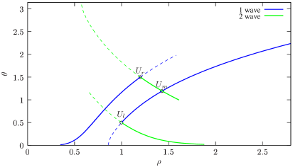
Figure 2: A solution of the Riemann problem with left and right states $U_{l}$ and $U_{r}$ (solid line for shock waves and dotted line for rarefaction waves). In this example, the solution is given by two shock waves.

3.3 The MV model as the relaxation limit of a conservative system

We are going to prove that the MV model (3.1)-(3.2)-(3.3) can be seen as the relaxation limit of a conservative hyperbolic model with a relaxation term. This link will be used later to build a new numerical scheme. More precisely, we introduce the relaxation model:

$$\displaystyle\partial_{t}\rho^{\varepsilon}+\nabla_{x}\cdot(\rho^{\varepsilon}\Omega^{\varepsilon})=0,$$ (3.20)

$$\displaystyle\partial_{t}\left(\rho^{\varepsilon}\Omega^{\varepsilon}\right)+c\nabla_{x}\cdot\left(\rho^{\varepsilon}\Omega^{\varepsilon}\otimes\Omega^{\varepsilon}\right)+\lambda\,\nabla_{x}\rho^{\varepsilon}=\frac{\rho^{\varepsilon}}{\varepsilon}(1-|\Omega^{\varepsilon}|^{2})\Omega^{\varepsilon}.$$ (3.21)

In this model, the constraint $|\Omega|=1$ is replaced by a relaxation operator. Formally, in the limit $\varepsilon\rightarrow 0$, we recover the constraint $|\Omega|=1$.

Proposition 3.1

The relaxation model (3.20)-(3.20) converges to the MV model (3.1)-(3.2)-(3.3) as $\varepsilon$ goes to zero.

Proof (formal). We define $R^{\varepsilon}=\rho^{\varepsilon}(1-|\Omega^{\varepsilon}|^{2})\Omega^{\varepsilon}$. Suppose that as $\varepsilon$ goes to zero:

$$\rho^{\varepsilon}\stackrel{{\scriptstyle\varepsilon\rightarrow 0}}{{\longrightarrow}}\rho^{0}\quad,\quad\Omega^{\varepsilon}\stackrel{{\scriptstyle\varepsilon\rightarrow 0}}{{\longrightarrow}}\Omega^{0}.$$ (3.22)

Then $R^{\varepsilon}\stackrel{{\scriptstyle\varepsilon\rightarrow 0}}{{\longrightarrow}}0$, which generically implies that $|\Omega^{0}|^{2}=1$ (except where $\rho^{0}\Omega^{0}=1$ which one assumes to be a negligible set). Therefore, we have:

$$\partial_{t}\Omega^{0}\cdot\Omega^{0}=0\quad,\quad(\Omega^{0}\cdot\nabla_{x})\Omega^{0}\,\cdot\Omega^{0}=0.$$ (3.23)

Then since $R^{\varepsilon}\times\Omega^{\varepsilon}=0$, we have:

$$(\partial_{t}\left(\rho^{\varepsilon}\Omega^{\varepsilon}\right)+c\nabla_{x}\cdot\left(\rho^{\varepsilon}\Omega^{\varepsilon}\otimes\Omega^{\varepsilon}\right)+\lambda\,\nabla_{x}\rho^{\varepsilon})\times\Omega^{\varepsilon}=0.$$

and consequently when $\varepsilon\rightarrow 0$:

$$\partial_{t}\left(\rho^{0}\Omega^{0}\right)+c\nabla_{x}\cdot\left(\rho^{0}\Omega^{0}\otimes\Omega^{0}\right)+\lambda\,\nabla_{x}\rho^{0}=\alpha\Omega^{0},$$ (3.24)

for a real number $\alpha$ to be determined. Taking the scalar product of (3.24) with $\Omega^{0}$ and using (3.23), we find:

$$\alpha=\partial_{t}\rho^{0}+c\nabla_{x}\cdot(\rho^{0}\Omega^{0})+\lambda\nabla_{x}\rho^{0}\cdot\Omega^{0}.$$

Using the conservation of mass ($\partial_{t}\rho^{0}=-\nabla_{x}\cdot(\rho^{0}\Omega^{0})$), we finally have:

$$\alpha=(c-1)\nabla_{x}\cdot(\rho^{0}\Omega^{0})+\lambda\nabla_{x}\rho^{0}\cdot\Omega^{0}.$$

Therefore, the relaxation term satisfies:

$$\frac{1}{\varepsilon}R^{\varepsilon}=[(c-1)\nabla_{x}\cdot(\rho^{0}\Omega^{0})+\lambda\nabla_{x}\rho^{0}\cdot\Omega^{0}]\Omega^{0}+O(\varepsilon).$$

Inserting in (3.20)-(3.21) and taking the limit $\varepsilon\rightarrow 0$, we recover the MV model (3.1)-(3.2) at the first order in $\varepsilon$.

$\Box$

Remark. As for the MV model, we can also analyze the hyperbolicity of the left hand side of (3.20)-(3.21). The eigenvalues are given by:

$$\gamma_{1}=cu-\sqrt{\Delta}\quad,\quad\gamma_{2}=cu\quad,\quad\gamma_{3}=cu+\sqrt{\Delta},$$

where $u$ denotes the $x$-coordinate of $\Omega$ and $\Delta=\lambda-(c-c^{2})u^{2}$. The system is hyperbolic if and only if $|u|<\sqrt{\frac{\lambda}{c-c^{2}}}$. As we can see in figure 3, for $u^{2}=1$, $\Delta$ is positive for any values of the noise parameter $d$. In particular, this implies that the relaxation model is hyperbolic for every $|u|\leq 1$.

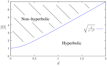
Figure 3: The quantity $\sqrt{\lambda/(c-c^{2})}$ depending on $d$. The relaxation model (3.20)-(3.20) is hyperbolic when the speed $|\Omega|$ is below this curve. At the limit $\varepsilon\rightarrow 0$, $|\Omega^{\varepsilon}|\rightarrow 1$ and therefore the relaxation model is hyperbolic for any $d$ in this limit.

4 Numerical simulations of the MV model

4.1 Numerical schemes

We propose four different numerical schemes to solve the MV model. The first two schemes originate from the discussions of the previous section, the two other one are based on the non-conservative form of the MV model.
We use the following notations: we fix a uniform stencil $(x_{i})_{i}$ (with $|x_{i+1}-x_{i}|=\Delta x$) and a time step $\Delta t$. We denote by $U_{i}^{n}=(\rho_{i}^{n},\,\theta_{i}^{n})$ the value of the mass and flux direction at the position $x_{i}$ and at time $n\Delta t$.

4.1.1 The conservative scheme

Here we use the conservative form of the MV model (3.15):

$$\partial_{t}V+\partial_{x}F(V)=0,$$ (4.25)

with $V=(\rho,f_{1}(\theta))^{T}$ and $F(V)=(\rho\cos\theta,\,cf_{2}(\theta)-\lambda\log(\rho))^{T}$. We use a Roe method to discretize this equation:

$$\frac{V_{i}^{n+1}-V_{i}^{n}}{\Delta t}+\frac{\widehat{F}_{i+}-\widehat{F}_{i-}}{\Delta x}=0,$$ (4.26)

where the intermediate flux $\widehat{F}_{i+}$ is given by:

$$\widehat{F}_{i+}=\frac{F(V_{i})+F(V_{i+1})}{2}\,-\left|\mathcal{A}(\overline{V}_{i+})\right|\frac{V_{i+1}-V_{i}}{2},$$ (4.27)

and $\mathcal{A}$ is the Jacobian of the flux $F$:

$$\mathcal{A}(V)=DF(V)=\left[\begin{array}[]{cc}\cos\theta&-\rho\sin^{2}\theta\\ -\frac{\lambda}{\rho}&c\cos\theta\end{array}\right]$$ (4.28)

calculated at the mean value $\overline{V}_{i+}=\frac{V_{i}+V_{i+1}}{2}.$

As mentioned earlier, the conservative form is only valid when $\theta$ does not cross a singularity $\theta=0$ or $\theta=\pi$ (i.e. $\sin\theta=0$). Nevertheless, numerically we can still use the formulation (4.26) when $\theta$ changes sign. Moreover, since $f_{1}$ is an even function, this only gives $|\theta^{n+1}|$. To determine the sign of $\theta^{n+1}$, we use an auxiliary value $\widehat{\theta}$ which we update with the upwind scheme (4.32). The sign of $\theta$ is then determined using the sign of $\widehat{\theta}$.

4.1.2 The splitting method

The next scheme uses the relaxation model (3.20)-(3.21). The idea is to split the relaxation model in two parts, first the conservative part:

$$\begin{array}[]{ll}&\displaystyle\partial_{t}\rho+\nabla_{x}\cdot(\rho\Omega)=0,\\ &\displaystyle\partial_{t}\left(\rho\Omega\right)+c\nabla_{x}\cdot\left(\rho\Omega\otimes\Omega\right)+\lambda\,\nabla_{x}\rho=0.\end{array}$$ (4.29)

and then the relaxation part:

$$\begin{array}[]{ccl}\displaystyle\partial_{t}\rho&=&0,\\ \displaystyle\partial_{t}\left(\rho\Omega\right)&=&\displaystyle\frac{\rho}{\varepsilon}(1-|\Omega|^{2})\Omega.\end{array}$$ (4.30)

This system reduces to: $\partial_{t}\Omega=\frac{1}{\varepsilon}(1-|\Omega|^{2})\Omega.$ Since this equation only changes the vector field $\Omega$ in norm (i.e. $\partial_{t}\Omega\cdot\Omega^{\perp}=0$), we can once again reduce this equation to:

$$\frac{1}{2}\partial_{t}|\Omega|^{2}=\frac{1}{\varepsilon}(1-|\Omega|^{2})|\Omega|^{2}.$$ (4.31)

Equation (4.31) can be explicitly solved: $|\Omega|^{2}\!=\!(1+C_{0}\,\mathrm{e}^{-2/\varepsilon\,t})^{-1}$ with $C_{0}\!=\!\left(\frac{1}{|\Omega_{0}|^{2}}-1\right)$. We indeed take the limit $\varepsilon\rightarrow 0$ of this expression and replace the relation term by a mere normalization: $\Omega\rightarrow\Omega/|\Omega|$ .

The conservative part is solved by a Roe method with a Roe matrix computed following [23] page 156.

4.1.3 Non-conservative schemes

We present two other numerical schemes based on the non-conservative formulation of the MV model.

(i) Upwind scheme

The method consists to update the value of $U_{i}^{n}$ with the formula:

$$\frac{U_{i}^{n+1}-U_{i}^{n}}{\Delta t}+A^{+}\left(\frac{U_{i}^{n}-U_{i-1}^{n}}{\Delta t}\right)+A^{-}\left(\frac{U_{i+1}^{n}-U_{i}^{n}}{\Delta t}\right)=0,$$ (4.32)

where $A^{+}$ and $A^{-}$ are (respectively) the positive and negative part of $A$, defined such that $A=A^{+}-A^{-}$ and $|A|=A^{+}+A^{-}$ and $A^{+},\,A^{-}$ are computed using an explicit diagonalization of $A$.

(ii) Semi-conservative scheme

One of the problem with the upwind scheme is that it does not conserve the total mass ($\int_{x}\rho(x)\,dx$). In order to keep this quantity constant in time, we use the equation of conservation of mass (3.1) in a conservative form:

$$\partial_{t}\rho+\partial_{x}H(\rho,\theta)=0,$$ (4.33)

with $H(\rho,\theta)=\rho\cos\theta$. Therefore, a conservative numerical scheme associated with this equation would be:

$$\frac{\rho_{i}^{n+1}-\rho_{i}^{n}}{\Delta t}+\frac{\widehat{H}_{i+1/2}-\widehat{H}_{i-1/2}}{\Delta x}=0,$$ (4.34)

where $\widehat{H}_{i+}$ is the numerical estimation of the flux $H$ at the interface between $x_{i}$ and $x_{i+1}$. To estimate numerically this flux, we use the following formula with $U_{i}=(\rho_{i},\theta_{i})$:

$$\widehat{H}_{i+1/2}=H(U_{i+1/2})-\left|A\right|_{\rho}\left(\frac{U_{i+1}^{n}-U_{i}^{n}}{2}\right),$$ (4.35)

where the intermediate value is given by $U_{i+1/2}=\frac{U_{i}^{n}+U_{i+1}^{n}}{2}$ and $\left|A\right|_{\rho}$ is the first line of the absolute value of $A$.

For the estimation of the angle $\theta$, we keep the same scheme as for the upwind scheme. This numerical scheme uses one conservative equation (for the mass $\rho$) and a non-conservative equation (for the angle $\theta$). It is thus referred to as the semi-conservative scheme.

4.2 Numerical simulations

To compare the various numerical schemes, we use a Riemann problem as initial condition. We choose solutions which consist of a rarefaction wave (figure 4) or a single shock wave (figures 5-6).

We take the following parameters: $d=1$, the length of the domain is $10$ units and the discontinuity for the Riemann problem is at $x=5$ (the middle of the domain). The simulations are run during two time units with a time step $\Delta t=2.10^{-2}$ and a space step $\Delta x=5.10^{-2}$. For these values, the Courant number ($C_{n}$) is $0.778$. We use homogeneous Neumann conditions as boundary conditions.

For the rarefaction wave, we take:

$$(\rho_{l},\theta_{l})=(2,1.7)\quad,\quad(\rho_{r},\theta_{r})=(1.12,0.60).$$ (4.36)

All the numerical schemes capture well the theoretical solution (see figure 4).

For the shock wave, we choose:

$$(\rho_{l},\theta_{l})=(1,1.05)\quad,\quad(\rho_{r},\theta_{r})=(1.432\,,\,1.7).$$ (4.37)

For these values, the shock speed computed with (3.2) is $s=-1.585$. The results of the numerical simulations using the four schemes are given in figure 5. The numerical solutions are in accordance with the theoretical solution given by the conservative formulation for all the numerical schemes. Nevertheless, the conservative scheme is in better accordance with this solution. For the other schemes, the shock speed differs slightly.
A second example of a shock wave is computed using the following initial condition:

$$(\rho_{l},\theta_{l})=(1,0.314)\quad,\quad(\rho_{r},\theta_{r})=(2,1.54).$$ (4.38)

The solutions given by the $4$ numerical schemes are very different. Only the conservative method is in agreement with the solution given by the conservative formulation. But the conservative formulation is not necessary the right one. Indeed, in the next section, particle simulations show that the right solution is not given by the conservative formulation but rather by the splitting method.

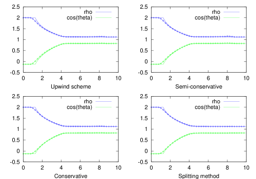
Figure 4: The theoretical solution of the Riemann problem (4.36) given by a rarefaction curve (solid line) and the numerical solutions (points), $\rho$ (blue) and $\cos\theta$ (green) as functions of space. The simulations are run during 2 time units, with a time step $\Delta t=2.10^{-2}$ and a space step $\Delta x=5.10^{-2}$ (CFL=$.778$).

Figure 5: Theoretical and numerical solutions of the Riemann problem (4.37)

Figure 6: Theoretical and numerical solutions of the Riemann problem (4.38)

5 The microscopic versus macroscopic Vicsek
models

5.1 Local equilibrium

In this part, we would like to validate the macroscopic Vicsek model by the simulation of the microscopic Vicsek. The macroscopic model relies on the fact that the particle distribution function is at local equilibrium given by a Von Mises distribution $M_{\Omega}$ (see [13]):

$$M_{\Omega}(\omega)=C\exp\left(\frac{\omega\cdot\Omega}{d}\right)$$ (5.1)

where $C$ is set by the normalization condition. The goal of this section is to show numerically that the particle distribution of the microscopic Vicsek model is close in certain regimes to this Von Mises distribution.

To this aim, in appendix C we propose a numerical scheme to solve system (2.2). The setting for our particle simulations is as follows: we consider a square box with periodic boundary conditions. As initial condition for the position $x_{i}$, we choose a uniform random distribution in space. The velocity is initially distributed according to a uniform distribution on the unit circle.

During the simulation, we compute the empirical distribution of the velocity direction $\theta$ and of the mean velocity $\Omega$ of particles. We then compare this empirical distribution with its theoretical distribution $M_{\Omega}(\theta)$ given by (5.1). In figure 7, we give an example of a comparison between the distribution of the velocity direction $\theta$ and the theoretical distribution $M_{\Omega}$ predicted by the theory.

Figure 7: Left figure: the distribution of velocity direction $\theta$ (with $\omega=(\cos\theta,\,\sin\theta)$) compared with its theoretical distribution after $6$ time units of simulation. Right figure: the corresponding particle simulation. Parameters of the simulation: $Lx=1$, $Ly=1$ (domain size), number of particles $N=500$, $\varepsilon=1/4$, $R=.5$, $d=.2$, $\Delta t=2.10^{-3}$.

Figure 8: The mean velocity $\varphi$ (5.2) for different values of $d$. Parameters of the simulation: $Lx=1$, $Ly=1$ (domain size), number of particles $N=200$, radius of interaction $R=.5$, $\Delta t=.02$ unit time, the simulations are run during $180$ unit time.

Since the distribution of velocity converges, we have a theoretical value for the mean velocity. We denote by $\varphi_{N}$ the mean velocity of particles and $\varphi$ the theoretical value given by the stationary distribution:

$$\varphi_{N}=\frac{1}{N}\left|\sum_{k=1}^{N}\omega_{k}\right|\quad,\quad\varphi=\left|\int_{\omega}\omega\,M_{\Omega}(\omega)\,d\omega\right|.$$ (5.2)

At least locally in $x$, we have that $\varphi_{N}\stackrel{{\scriptstyle\epsilon\rightarrow 0}}{{\longrightarrow}}\varphi$. In figure 8, we compare the two distributions for different values of the noise $d$ and we can see that the two distributions are in good agreement. We also observe a smooth transition from order ($\varphi\approx 1$) to disorder ($\varphi<<1$) as it has been measured in the original Vicsek model [29].

The situation is different when we look at a larger system. We still have convergence of the velocity distribution of particles to a local equilibrium $\rho(x)\,M_{\Omega(x)}(\omega)$, but the mean direction $\Omega(x)$ now depends on $x$. Therefore the mean velocity of the particles in all the domain differs from the expected theoretical value (5.1)-(5.2). We illustrate this phenomena in figure 9: we fix the density of particles and we increase the size of the box. As we can observe, the mean velocity $\varphi_{N}$ (5.2) has a smaller value when the size of the box increases. This phenomena has been previously observed in [7]. The mean velocity $\varphi_{N}$ can also differ from the expected theoretical value $\varphi$ (5.1)-(5.2) when the density of particles is low. In figure 10, we fix the size of the box ($L=10$) and we increase the density of particles (the density is given by the number of particles inside the circle of interaction). At low density, the mean velocity $\varphi_{N}$ is much more smaller than the theoretical prediction $\varphi$. But as the density of particles increases, the mean velocity $\varphi_{N}$ grows (see also [29]) and moreover $\varphi_{N}$ converges to $\varphi$. Because of that, a dense regime of particles has to be used in the following in order to numerically compare the microscopic model with the MV model.

Figure 9: The mean velocity $\varphi$ (5.2) for different values of $d$. We use different domain sizes and we keep the same density of particles. As the domain size increases, the total flux $\varphi$ decreases which means that particles are less aligned globally. Parameters of the simulations: $L=1,\,2,\,5,\,10$ (domain size), number of particles $N=200,\,800,\,5000,\,20000$, radius of interaction $R=.5$, $\Delta t=.02$ time units, the simulations are run during $180$ time units.

Figure 10: The mean velocity $\varphi$ (5.2) for different values of $d$. We change the density of particles (given by the mean number of neighbors in unit of radius of interaction). When we increase the mean number of neighbors, particles are more aligned. Parameters of the simulations: $L=10$ (domain size), number of particles $N=254,\,1273,\,6366,\,12732,$ and $25464$, radius of interaction $R=.5$, $\Delta t=.02$ time units, the simulations are run during $180$ time units.

5.2 Microscopic versus Macroscopic dynamics

We now compare the evolution of the two macroscopic quantities $\rho$ and $\Omega$ for the two models. We have seen that the different schemes applied to the macroscopic equation can give different solutions (see figure 6). Therefore, we expect that particle simulations will indicate what is the physically relevant solution of the macroscopic equation.

We first briefly explain how we proceed to run the particle simulations of a Riemann problem (see also appendix C). First, we have to choose a left state $(\rho_{l},\theta_{l})$, a right state $(\rho_{r},\theta_{r})$ and the noise parameter $d$. Then we distribute a proportion $\frac{\rho_{l}}{\rho_{l}+\rho_{r}}$ of particles uniformly in the interval $[0,5]$ and the remaining particles uniformly in the interval $[5,10]$. Then, we generate velocity distribution $\theta$ for the particles according to the distribution $M_{\Omega}$ (5.1) with $\Omega_{l}=(\cos\theta_{l},\sin\theta_{l})^{T}$ on the left side and $\Omega_{r}=(\cos\theta_{r},\sin\theta_{r})^{T}$ on the right side. We use the numerical scheme given in appendix C to generate particle trajectories. To make the computation simpler, we choose periodic boundary conditions. Therefore the number of particles is conserved. As a consequence, there are two Riemann problems corresponding to discontinuities at $x=5$ and at $x=0$ or $10$ (which is the same by periodicity). We use a particle-in-cell method [15, 19] to estimate the two macroscopic quantities: the density $\rho$ and the direction of the flux $\Omega$ (which gives $\theta$). In order to reduce the noise due to the finite number of particles, we take a mean over several simulations to estimate the density $\rho$ and $\theta$ ($10$ simulations in our examples).

In figure 11, we show a numerical solution for the following Riemann problem:

$$(\rho_{l},\,\theta_{l})=(1,\,1.5)\quad,\quad(\rho_{r},\,\theta_{r})=(2,\,1.83)\quad,\quad d=0.2$$ (5.3)

using particle simulations and the macroscopic equation. We represent the solutions in a 2D representation. Since the initial condition is such that the density $\rho$ and the direction $\theta$ are independent of the $y$-direction, we only represent $\rho$ and $\theta$ along the $x$-axis in the following figures.

In figure 12, we represent the two solutions (the particle and the macroscopic one) with only a dependence in the $x$-direction. Three quantities are represented: the density (blue), the flux direction $\theta$ (green) and the variance of the angle distribution (red). The macroscopic model supposes that the variance of $\theta$ should be constant everywhere. Nevertheless, we can see that the variance is larger in regions where the density is lower. For $\rho$ and $\theta$, we see clearly the propagation of a shock in the middle of the domain and a rarefaction at the boundary. The CPU time for one numerical solution at the particle level is about $140$ seconds with the parameters given in figure 12. For the macroscopic equation, the CPU time is about $0.1$ second which represents a cost reduction of three orders of magnitude compared with the particle simulations. Since we have to take a mean over many particle simulations, the cost reduction is even larger.

In figure 13, we use the same Riemann problem to set the initial position as in figure 6 both with $d=1$ (4.38). We use a larger domain in $x$ ($L=20$ space units) in order to avoid the effect of the periodic boundary condition. The upwind scheme and the semi-conservative method are clearly not in accordance with the particle simulations. Moreover, the splitting method is in better agreement with the particle simulation since the shock speed is closer to the values given by the particle simulations than that predicted by the conservative scheme.

Finally, our last simulations concern a contact discontinuity. We simply initialize with:

$$(\rho_{l},\theta_{l})=(1,1)\quad,\quad(\rho_{r},\theta_{r})=(1,-1)\quad,\quad d=0.2,$$ (5.4)

i.e. we reflect the angle with respect to the x-axis across the middle point $x=5$. A natural solution for this problem is the contact discontinuity propagating at speed $c\,cos(1)$:

$$\rho(t,x)=1\quad,\quad\theta(t,x)=\theta_{0}(x-c\cos(1)t),$$ (5.5)

with $\theta_{0}(x)=-1$ when $x<5$ and $\theta_{0}(x)=1$ when $x>5$. This is the solution provided by the conservative scheme (figure 14). But surprisingly, the splitting method and the particle simulation agree on a different solution. Indeed, the solutions given by the particles and the splitting method are in fairly good agreement with each other, which seems to indicate that the “physical solution” to the contact problem (5.4) is not given by the conservative formulation (5.5) but by a much more complex profile. The constraint of unit speed drastically changes the profile of the solution compared with what would be found for a standard system of conservative laws.

Figure 11: The particle density in space $\rho$ computed with particle simulations (left) and the macroscopic equations (right). We initialize with a Riemann problem (5.3). Numerical parameters for the particle simulations: $N=2.10^{6}$ particles, $\Delta t=.01$, $\varepsilon=1/10$, $R=.5$, $Lx=Ly=10$, we take a mean over $10$ computations. Numerical parameters for the macroscopic model: $\Delta t=.01,\,\Delta x=.025$ (CFL=0.416), we use the splitting method. The simulations are run during 2 time units.

Figure 12: The solution of the Riemann problem (5.3) with $d=.2$ computed with the splitting method (solid line) and with particle simulations (dots). In blue, we represent the density $\rho$, in green the flux direction $\theta$ and in red the variance of the velocity direction. The parameters are the same as in figure 11. We only change the representation of the solution (1D-representation).

Figure 13: The solutions of the Riemann problem (4.38) with $d=1$ computed using the macroscopic model and particle simulations of the microscopic model (see figure 12). Numerical parameters for the macroscopic model: $\Delta t=.01,\,\Delta x=.025$ (CFL=0.778). Numerical parameters for the particle simulation: $N=2.10^{6}$ particles, $\Delta t=.02$, $\varepsilon=.1$, $R=.5$, $Lx=20$ and $Ly=1$. We take a mean over $50$ simulations. The simulations are run during 6 time units. Since $d=1$, fluctuations are higher (see figure 9), we have to increase the density of particles to reduce this effect.

Conservative method

Splitting method

Figure 14: The solution of the Riemann problem (5.4) computed with the conservative method (top), the splitting method (down) and with particle simulations (dots). Numerical parameters for the macroscopic model: $\Delta t=.01,\,\Delta x=.025$ (CFL=0.416). Numerical parameters for the particle simulations: $N=10^{6}$ particles, $\Delta t=.01$, $\varepsilon=1/10$, $R=.5$, $Lx=10$, $Ly=1$. We take a mean over $100$ simulations. The simulations are run during 2 time units.

6 Conclusion

In this work, we have numerically studied both the microscopic Vicsek model and its macroscopic version [13]. Due to the geometric constraint that the velocity should be of norm one, the standard theory of hyperbolic systems is not applicable. Therefore, we have proposed several numerical schemes to solve it. By comparing the numerical simulations of the microscopic and macroscopic equations, it appears that the scheme based on a relaxation formulation of the macroscopic model, used in conjunction with a splitting method is in good agreement with particle simulations. The other schemes do not show a similar good agreement. In particular, with an initial condition given by a contact discontinuity, the splitting method and the microscopic model provide a similar solution which turn to be much more complex than what we could be expected.

These results confirm the relevance of the macroscopic Vicsek model. Since the CPU time is much lower with the macroscopic equation, the macroscopic Vicsek model is an effective tool to simulate the Vicsek dynamics in a dense regime of particles.

Many problems are still open concerning the macroscopic Vicsek model. We have seen that the splitting method gives results which are in accordance with particle simulations. But, we have to understand why this particular scheme captures well the particle dynamics better than the other schemes. Since the macroscopic equation has original characteristics, this question is challenging. Another point concerns the particle simulations. We have seen that the particles density has a strong effect on the variance of the velocity distribution. When the density is low, the variance is larger. The macroscopic equation does not capture this effect since the variance of the distribution is constant. Works in progress aims at taking into account this density effect.

Appendix A The coefficients $c_{1}$, $c_{2}$ and $\lambda$

The analytical expression of the coefficient $c_{1}$ involved the distribution of the local equilibrium $M_{\Omega}$ (5.1). The two other coefficients ($c_{2}$ and $\lambda$) involve also the solution $g$ of the following elliptic equation [13]:

$$-(1-x^{2})\,\partial_{x}[\mathrm{e}^{x/d}(1-x^{2})\partial_{x}g]+\mathrm{e}^{x/d}g=-(1-x^{2})^{3/2}\mathrm{e}^{x/d},$$ (A.1)

on the interval $x\in(-1,1)$.

If we define the function $h=\frac{g}{\sqrt{1-x^{2}}}$ and $M(x)=\mathrm{e}^{\frac{x}{d}}$, these macroscopic coefficients can be written as:

$$c_{1} = <\cos\theta>|_{M}=\frac{\int_{0}^{\pi}\cos\theta\,M(\cos\theta)\sin\theta\,d\theta}{\int_{0}^{\pi}M(\cos\theta)\sin\theta\,d\theta},$$ (A.2)

$$c_{2} = <\cos\theta>|_{\sin^{2}\theta\,hM}=\frac{\int_{0}^{\pi}\cos\theta\,\sin^{2}\theta\,h(\cos\theta)M(\cos\theta)\sin\theta\,d\theta}{\int_{0}^{\pi}\sin^{2}\theta\,h(\cos\theta)M(\cos\theta)\sin\theta\,d\theta},$$ (A.3)

$$\lambda = d.$$ (A.4)

In the above expressions, we can see that $0\leq c_{1},c_{2}\leq 1$.

Now we are going to explore two asymptotics of $g$ when the parameter $d$ is small or large.

Lemma A.1

Let $g$ be the solution of equation (A.1). We have the asymptotics:

$$g \stackrel{{\scriptstyle d\rightarrow 0}}{{\sim}} d\left[\text{asin}(x)-\frac{\pi}{2}\right]+o(d),$$ (A.5)

$$g \stackrel{{\scriptstyle d\rightarrow\infty}}{{\sim}} -\frac{1}{2}\,\sqrt{1-x^{2}}+\frac{1}{12\,d}x\sqrt{1-x^{2}}+o\left(\frac{1}{d}\right).$$ (A.6)

Proof (formal). Introducing the Hilbert space:

$$V=\{g\,|\,(1-\mu^{2})^{-1/2}g\in L^{2}(-1,1),\quad(1-\mu^{2})^{1/2}\partial_{\mu}g\in L^{2}(-1,1)\}$$

we have already seen in [13] that there exists a unique solution $g$ of (A.1). Moreover this solution is negative.

To derive the asymptotic behavior of $g$ depending on $d$, we first develop (A.1):

$$\partial_{x}[(1-x^{2})\partial_{x}g]+(1-x^{2})\,\frac{1}{d}\partial_{x}g-\frac{g}{1-x^{2}}=(1-x^{2})^{1/2}.$$ (A.7)

When $d\rightarrow 0$, we have:

$$\partial_{x}g=0$$

on the interval $[-1+\varepsilon,1-\varepsilon]$ for all $\varepsilon>0$. Since $g$ belongs to $V$, we also have the boundary condition $g(-1)=g(1)=0$, so $g$ converges to $0$ when $d\rightarrow 0$.
To derive the next order of convergence in the limit $d\rightarrow 0$, we normalize $g$ with $g=d\widetilde{g}$, which gives:

$$d\,\partial_{x}[(1-x^{2})\partial_{x}\widetilde{g}]+(1-x^{2})\partial_{x}\widetilde{g}-d\,\frac{\widetilde{g}}{1-x^{2}}=(1-x^{2})^{1/2}.$$ (A.8)

In the limit $d\rightarrow 0$, we deduce that:

$$(1-x^{2})\partial_{x}\widetilde{g}=(1-x^{2})^{1/2},$$ (A.9)

which has an explicit solution: $\widetilde{g}=\text{asin}(x)+c$. Since $\widetilde{g}\leq 0$, we have $c\leq-\frac{\pi}{2}$. Numerically, we find that $c=-\frac{\pi}{2}$ but the proof is still open. This formally proves (A.5).

When $d\rightarrow+\infty$, (A.7) gives:

$$\partial_{x}[(1-x^{2})\partial_{x}g_{0}]-\frac{g_{0}}{1-x^{2}}=(1-x^{2})^{1/2}.$$ (A.10)

A simple calculation shows that $g_{0}=-\frac{1}{2}\,\sqrt{1-x^{2}}$ is a solution of (A.10).
To derive the next order of convergence, we look at the difference $v=d(g-g_{0})$, which satisfies (see (A.7) and (A.10)):

$$\partial_{x}[(1-x^{2})\partial_{x}v]+(1-x^{2})\,\frac{1}{d}\partial_{x}v-\frac{v}{1-x^{2}}=-(1-x^{2})\,\partial_{x}g_{0}.$$

In the limit $d\rightarrow+\infty$, $v$ satisfies:

$$\partial_{x}[(1-x^{2})\partial_{x}v]-\frac{v}{1-x^{2}}=-\frac{1}{2}x\sqrt{1-x^{2}}.$$ (A.11)

A simple calculation shows that $v=\frac{1}{12}x\sqrt{1-x^{2}}$ is solution of (A.11). Therefore we formally have the expression (A.6) in the proposition.

$\Box$

In figure 15, we compute numerically the function $g$ (A.1). We use a finite element method with a space step $\Delta x=10^{-3}$. The two asymptotics of $g$ when $d\rightarrow 0$ and $d\rightarrow+\infty$ are computed in figure 16.

Proposition A.2

The two coefficients $c_{1}$ and $c_{2}$ defined (resp.) by the equations (A.2) and (A.3) satisfy the following asymptotics:

$$c_{1} \stackrel{{\scriptstyle d\rightarrow 0}}{{\sim}} 1-d+O(d^{2}),$$ (A.12)

$$c_{1} \stackrel{{\scriptstyle d\rightarrow+\infty}}{{\sim}} \frac{1}{3d}+O\left(\frac{1}{d^{2}}\right),$$ (A.13)

$$c_{2} \stackrel{{\scriptstyle d\rightarrow\infty}}{{\sim}} \frac{1}{6d}+o\left(\frac{1}{d}\right).$$ (A.14)

Proof.

We have an explicit expression for the coefficient $c_{1}$ using the change of unknowns $x=\cos(\theta)$:

$$c_{1} = \text{coth}\left(\frac{1}{d}\right)-d,$$ (A.15)

where $\text{coth}(s)=\frac{\mathrm{e}^{s}+\mathrm{e}^{-s}}{\mathrm{e}^{s}-\mathrm{e}^{-s}}$. The expressions of (A.12) and (A.13) are simply deduced by a Taylor expansion of the last expression.

For the coefficient $c_{2}$, we insert the development of $g$ (A.6) in expression (A.3). ∎

Remark. The behavior of $c_{2}$ when $d\rightarrow 0$ is more difficult to analyze. The density probability $\sin\theta\,h\,M$ used in formula (A.3) becomes singular in this limit. Nevertheless, due to the expression of $M_{\Omega}$, the density converges to a Dirac delta at $0$ which explains why $c_{2}\stackrel{{\scriptstyle d\rightarrow 0}}{{\sim}}1$. To capture the next order of convergence, we need to find the second order correction of $g$ in the limit $d\rightarrow 0$ which is not available. However, numerically we find that:

$$c_{2}\stackrel{{\scriptstyle d\rightarrow 0}}{{\sim}}1-2d+o(d).$$

In figure 17, we numerically compute the coefficients $c_{2}/c_{1}$, $\lambda/c_{1}$ and their asymptotics.

Figure 15: The numerical solution $g$ of (A.1) for different values of the parameter $d$. We have the following asymptotics (see lemma A.1): $g\stackrel{{\scriptstyle d\rightarrow 0}}{{\longrightarrow}}0$ and $g\stackrel{{\scriptstyle d\rightarrow\infty}}{{\longrightarrow}}-\frac{1}{2}\sqrt{1-x^{2}}$.

Figure 16: Left figure: the first correction $g_{1}$ of $g$ when $d\rightarrow 0$. The red curve is the theoretical asymptotic limit: $g_{1}=g/d\stackrel{{\scriptstyle d\rightarrow 0}}{{\longrightarrow}}\text{asin}(x)-\frac{\pi}{2}$ (see lemma A.1). Right figure: the first correction $g_{1}$ of $g$ when $d\rightarrow+\infty$. The red curve is the theoretical asymptotic: $g_{1}=d(g+\frac{1}{2}\,\sqrt{1-x^{2}})\stackrel{{\scriptstyle d\rightarrow 0}}{{\longrightarrow}}\frac{1}{12}x\sqrt{1-x^{2}}$ (see lemma A.1).

Figure 17: The ratio $c_{2}/c_{1}$ and $\lambda/c_{1}$ (solid lines) and their two asymptotics (dashed lines) (see proposition A.2) computed with $\Delta x=10^{-3}$.

Appendix B Special solution of the MV model

In this appendix, a vortex configuration is exhibited as a stationary solution of the MV model (2.4)-(2.5)-(2.6) in dimension 2. A stationary state of the MV model has to satisfy:

$$\begin{array}[]{ll}&\nabla_{x}\cdot(\rho\Omega)=0,\\ &c(\Omega\cdot\nabla_{x})\Omega+\lambda\,(\mbox{Id}-\Omega\otimes\Omega)\frac{\nabla_{x}\rho}{\rho}=0.\end{array}$$ (B.1)

Introducing the polar coordinates, $\rho(r,\theta)$, $\Omega(r,\theta)=f_{r}(r,\theta)\vec{e}_{r}+f_{\theta}(r,\theta)\vec{e}_{\theta}$, where $\vec{e}_{r}=\left(\cos\theta,\sin\theta\right)^{T}$ and $\vec{e}_{\theta}=\left(-\sin\theta,\cos\theta\right)^{T}$, we are able to formulate the proposition:

Proposition B.1

The following initial condition is a stationary state of the MV model (B.1):

$$\rho(r)=C\,r^{c/\lambda}\qquad,\qquad\Omega=\vec{e}_{\theta},$$ (B.2)

where $C$ is a constant.

Proof.

With the expression of $\rho$ and $\Omega$ given by (B.2), the divergence of the mass is zero and the gradient of $\rho$ is orthogonal to $\Omega$, therefore the system (B.1) reduces to:

$$c(\Omega\cdot\nabla_{x})\Omega+\lambda\frac{\nabla_{x}\rho}{\rho}=0,$$ (B.3)

or in polar coordinates:

$$c\frac{1}{r}\partial_{\theta}\,\vec{e}_{\theta}\,+\,\lambda\frac{\rho^{\prime}(r)}{\rho(r)}\vec{e}_{r}=0.$$

Since $\partial_{\theta}\vec{e}_{\theta}=-\vec{e}_{r}$, we can easily check that the solution of this equation is given by $\rho(r)=C\,r^{c/\lambda}$. ∎

Appendix C Numerical schemes for particle simulations

In the limit $\varepsilon\rightarrow 0$, an explicit Euler method for the differential system (2.1)-(2.2) imposes a restriction time step condition of $\frac{1}{\varepsilon}\Delta t<1$. Therefore, we develop an implicit scheme for this system. The idea is to go back to the original Vicsek model (see [13]). We use the formulation:

$$\frac{\omega^{n+1}-\omega^{n}}{\Delta t}=(\mbox{Id}-\omega^{n+1/2}\otimes\omega^{n+1/2})(\bar{\omega}^{n}-\omega^{n})$$ (C.1)

where $\omega^{n+1/2}=\frac{\omega^{n}+\omega^{n+1}}{|\omega^{n}+\omega^{n+1}|}$ and $\bar{\omega}^{n}$ is the average velocity (2.3). When $\Delta t=1$, we recover exactly the original Vicsek model [29]. (C.1) can in fact be solved explicitly. First, we have to remember that $\omega^{n+1}$ belongs to the unit circle (i.e. $|\omega^{n+1}|=1$). Then we use that $\omega^{n+1}-\omega^{n}$ is the orthogonal projection of $(\bar{\omega}^{n}-\omega^{n})\Delta t$ on the orthogonal plan of $\omega^{n+1/2}$. Therefore $\omega^{n+1}$ and $\omega_{n}$ are on the circle $\mathcal{C}$ with center $B=\omega_{n}+\frac{(\bar{\omega}^{n}-\omega^{n})\Delta t}{2}$ and radius $\left|\frac{(\bar{\omega}^{n}-\omega^{n})\Delta t}{2}\right|$ (see figure 18). This fully defines $\omega^{n+1}$ since $\omega^{n}$ and $\omega^{n+1}$ are the two intersection points of the unit circle and the circle $\mathcal{C}$. Denoting $\theta$ the angle of the unit vector $\omega$, we easily check that we have in terms of angles:

$$\theta^{n+1}=\theta^{n}+2\widehat{(\omega^{n},B)}.$$

To take into account the effect of the noise, we simply add a random variable:

$$\theta^{n+1}=\theta^{n}+2\widehat{(\omega^{n},B)}+\sqrt{2d\,\Delta t}\,\epsilon_{n}$$ (C.2)

where $\epsilon_{n}$ is a standard normal distribution independent of $\theta^{n}$.

Figure 18: Illustration of the geometric method to solve explicitly equation (C.1).

Algorithm used to solve a Riemann problem with particles.

1. Choose a Riemann problem $(\rho_{l},\,\theta_{l})$ and $(\rho_{r},\,\theta_{r})$.

2. Initiate $N$ particles $(x_{k},\omega_{k})_{k=1..N}$ according to the distributions $\rho_{l}M_{\Omega_{l}}$ and $\rho_{r}M_{\Omega_{r}}$.

3. Let evolve the particles in time using the time-discretization (C.2) of equation (2.2).

4. Compute the mass $\rho$ and the direction of the flux $\Omega$ using Particle-In-Cell method [19] in order to compare the simulation with the one of the MV model.

References

- [1] M. Aldana and C. Huepe. Phase Transitions in Self-Driven Many-Particle Systems and Related Non-Equilibrium Models: A Network Approach. Journal of Statistical Physics, 112(1):135–153, 2003.
- [2] I. Aoki. A simulation study on the schooling mechanism in fish. Bulletin of the Japanese Society of Scientific Fisheries (Japan), 1982.
- [3] M. Ballerini, N. Cabibbo, R. Candelier, A. Cavagna, E. Cisbani, I. Giardina, V. Lecomte, A. Orlandi, G. Parisi, A. Procaccini, et al. Interaction ruling animal collective behavior depends on topological rather than metric distance: Evidence from a field study. Proceedings of the National Academy of Sciences, 105(4):1232, 2008.
- [4] E. Bertin, M. Droz, and G. Grégoire. Boltzmann and hydrodynamic description for self-propelled particles. Physical Review E, 74(2):22101, 2006.
- [5] F. Bouchut. Nonlinear stability of finite volume methods for hyperbolic conservation laws and well-balanced schemes for sources. Birkhauser, 2004.
- [6] J. Buhl, DJT Sumpter, ID Couzin, JJ Hale, E. Despland, ER Miller, and SJ Simpson. From disorder to order in marching locusts, 2006.
- [7] H. Chaté, F. Ginelli, G. Grégoire, and F. Raynaud. Collective motion of self-propelled particles interacting without cohesion. Physical Review E, 77(4):46113, 2008.
- [8] GQ Chen, CD Levermore, and TP Liu. Hyperbolic conservation laws with sti relaxation and entropy. Comm. Pure Appl. Math, 47:787, 1994.
- [9] Y. Chuang, M.R. D’Orsogna, D. Marthaler, A.L. Bertozzi, and L.S. Chayes. State transitions and the continuum limit for a 2d interacting, self-propelled particle system. Physica D: Nonlinear Phenomena, 232(1):33–47, 2007.
- [10] I.D. Couzin, J. Krause, R. James, G.D. Ruxton, and N.R. Franks. Collective memory and spatial sorting in animal groups. Journal of Theoretical Biology, 218(1):1–11, 2002.
- [11] F. Cucker and E. Mordecki. Flocking in noisy environments. Journal de mathématiques pures et appliquées, 2007.
- [12] F. Cucker and S. Smale. Emergent behavior in flocks. IEEE Transactions on automatic control, 52(5):852, 2007.
- [13] P. Degond and S. Motsch. Macroscopic limit of self-driven particles with orientation interaction. Comptes rendus-Mathématique, 345(10):555–560, 2007.
- [14] P. Degond and S. Motsch. Large scale dynamics of the persistent turning walker model of fish behavior. Journal of Statistical Physics, 131(6):989–1021, 2008.
- [15] H. Fehske, R. Schneider, and A. Weisse. Computational Many-Particle Physics. Springer Verlag, 2007.
- [16] J. Gautrais, C. Jost, M. Soria, A. Campo, S. Motsch, R. Fournier, S. Blanco, and G. Theraulaz. Analyzing fish movement as a persistent turning walker. Journal of Mathematical Biology, 58(3):429–445, 2009.
- [17] G. Grégoire and H. Chaté. Onset of collective and cohesive motion. Physical Review Letters, 92(2):25702, 2004.
- [18] S. Y Ha and E. Tadmor. From particle to kinetic and hydrodynamic descriptions of flocking. Kinetic and Related Models, 3(1):415–435, 2008.
- [19] R.W. Hockney and J.W. Eastwood. Computer Simulation Using Particles. Institute of Physics Publishing, 1988.
- [20] A. Huth and C. Wissel. The simulation of the movement of fish schools. Journal of theoretical biology, 156(3):365–385, 1992.
- [21] P.L. LeFloch. Entropy weak solutions to nonlinear hyperbolic systems under nonconservative form. Communications in Partial Differential Equations, 13(6):669–727, 1988.
- [22] R.J. LeVeque. Numerical Methods for Conservation Laws. Birkhäuser, 1992.
- [23] R.J. LeVeque and MyiLibrary. Finite volume methods for hyperbolic problems. Cambridge University Press, 2002.
- [24] A. Mogilner and L. Edelstein-Keshet. A non-local model for a swarm. Journal of Mathematical Biology, 38(6):534–570, 1999.
- [25] M. Nagy, I. Daruka, and T. Vicsek. New aspects of the continuous phase transition in the scalar noise model (SNM) of collective motion. Physica A: Statistical Mechanics and its Applications, 373:445–454, 2007.
- [26] C.W. Reynolds. Flocks, herds and schools: A distributed behavioral model. pages 25–34, 1987.
- [27] AS Sznitman. Topics in propagation of chaos. Ecole d’été de probabilités de Saint-Flour XIX-1989. Lecture Notes in Math, 1464:165–251, 1989.
- [28] E.F. Toro. Riemann solvers and numerical methods for fluid dynamics. Springer New York, 1997.
- [29] T. Vicsek, A. Czirók, E. Ben-Jacob, I. Cohen, and O. Shochet. Novel type of phase transition in a system of self-driven particles. Physical Review Letters, 75(6):1226–1229, 1995.