Structure of even-even nuclei using a mapped collective Hamiltonian and the D1S Gogny interaction

Abstract

A systematic study of low energy nuclear structure at normal deformation is carried out using the Hartree-Fock-Bogoliubov theory extended by the Generator Coordinate Method and mapped onto a 5-dimensional collective quadrupole Hamiltonian. Results obtained with the Gogny D1S interaction are presented from dripline to dripline for even-even nuclei with proton numbers $Z=10$ to $Z=110$ and neutron numbers N $\leq$ 200. The properties calculated for the ground states are their charge radii, 2-particle separation energies, correlation energies, and the intrinsic quadrupole shape parameters. For the excited spectroscopy, the observables calculated are the excitation energies and quadrupole as well as monopole transition matrix elements. We examine in this work the yrast levels up to $J=6$, the lowest excited $0^{+}$ states, and the two next yrare $2^{+}$ states. The theory is applicable to more than 90% of the nuclei which have tabulated measurements. We assess its accuracy by comparison with experiments on all applicable nuclei where the systematic tabulations of the data are available. We find that the predicted radii have an accuracy of 0.6%, much better than can be achieved with a smooth phenomenological description. The correlation energy obtained from the collective Hamiltonian gives a significant improvement to the accuracy of the 2-particle separation energies and to their differences, the 2-particle gaps. Many of the properties depend strongly on the intrinsic deformation and we find that the theory is especially reliable for strongly deformed nuclei. The distribution of values of the collective structure indicator $R_{42}={E(4^{+}_{1})}/{E(2^{+}_{1})}$ has a very sharp peak at the value 10/3, in agreement with the existing data. On average, the predicted excitation energy and transition strength of the first $2^{+}$ excitation are 12 % and 22% higher than experiment, respectively, with variances of the order of 40-50 %. The theory gives a good qualitative account of the range of variation of the excitation energy of the first excited $0^{+}$ state, but the predicted energies are systematically 50 % high. The calculated yrare $2^{+}$ states show a clear separation between $\gamma$ and $\beta$ excitations, and the energies of the $2^{+}$ $\gamma$-vibrations accord well with experiment. The character of the $0^{+}_{2}$ state is interpreted as shape coexistence or $\beta$-vibrational excitations on the basis of relative quadrupole transition strengths. Bands are predicted with the properties of $\beta$-vibrations for many nuclei having $R_{42}$ values corresponding to axial rotors, but the shape coexistence phenomenon is more prevalent. The data set of the calculated properties of 1712 even-even nuclei, including spectroscopic properties for 1693 of them, are provided in CEA website and EPAPS repository with this article epaps .

I Introduction

A present-day goal in nuclear theory is to develop a universal theory of nuclear structure, in the sense that it is well-founded in its methodology and is applicable across the chart of nuclides. The most promising starting point is self-consistent mean-field, but the theory must be extended in some way to treat excitations and nuclear spectroscopy. For any candidate theory or methodology, one needs to know its performance on known observables to be confident about predictions to unknown nuclei or regions of the nuclear chart. It is our purpose to provide and document this information for one particular theory, the constrained-Hartree-Fock-Bogoliubov (CHFB) theory together with a mapping to the five-dimensional collective Hamiltonian (5DCH), using the Gogny D1S interaction in the nuclear Hamiltonian De80 ; Be91 . The results presented here are a major extension of the our study of one particular observable in the CHFB+5DCH theory, the low-lying quadrupole excitation be07 . Since that work and during the course of the present calculations two new parameterizations of the Gogny force have been published hilaire . These are aimed at removing systematic deviations of calculated binding energies from measurements using the D1S force. However, for our purposes, the global assessment of spectroscopy properties, it is more important at this stage to benchmark the predictions of a stable and widely tested Hamiltonian. The present results will therefore serve as a baseline for comparisons with the next generation of similar structure calculations based on the new parameterizations. We mention that the present era of global calculations within self-consistent mean field theory using a fixed interaction started with the calculations of Tajima et al. ta96 and Lalazissis et al. La96 . Also, the mapping to 5DCH has recently been adapted and applied to the Skyrme and the relativistic mean-field Hamiltonians kl08 ,ni09 .

The CHFB+5DCH theory is one of several paths that could be taken to extend mean-field theory to describe spectroscopic properties such as excitation energies. Rather than constructing a collective Hamiltonian from the CHFB solutions, the constrained wave functions may be projected on good angular momentum and then used directly to construct a discrete basis Hamiltonian. This technology in now fairly well developed Bonche ; Robledo and has recently been applied to the global study of correlation energies Ben06 and the lowest $2^{+}$ excitations sa07 . In principle, it should give similar results to the CHFB+5DCH theory applying the same Hamiltonian. However, in the present implementations the discrete-basis wave functions do not include triaxial deformations and the effective rotational inertias arising from the Hamiltonian matrix element are not self-consistent. On the other hand, discrete basis methods do not rely on the Gaussian Overlap Approximation which we require for our Hamiltonian mapping. There is a third path to introduce dynamics into mean field theory, the quasi-particle random-phase approximation (QRPA). That has also been applied to many nuclei, but so far global surveys have been restricted to spherical nuclei te08 .

The methodology in the present work has two stages, the CHFB calculations to set up the 5DCH input, and the solution of the 5DCH equations. For the first part, we perform CHFB calculations on a large triaxial grid of quadrupole deformations. These provide a potential energy surface and the inertial masses needed for the 5DCH. Positive parity solutions are extracted for about 1700 even-even nuclei with proton numbers Z = 10 to Z = 110 and neutron numbers N $\leq$ 200. These calculations span most of the periodic table from drip-line to drip-line. One purpose of our work is to establish benchmarks for the accuracy and reliability of the theory for energies and properties of the low excitations. We therefore make systematic comparisons with experimental data, especially when it is available as a tabulation from a published critical review or data repository. The quantities that we can easily compare are two-nucleon separation energies and gaps, excitation energies of the lowest excited states including yrast spectra up to $J=6$, and transition rates of the lowest $2^{+}$ and excited $0^{+}$ states. Since no effective charge is involved, our predictions are free of parameters beyond those contained in the Gogny D1S interaction. We hope these calculations will be helpful to understand the limitations of the theory and ultimately find improved methodologies and Hamiltonians. One important question deals with shell gaps and magic numbers. Far from stability, dedicated experiments have shown that the N = 20, 28 shell gaps experience erosion and that N = 16 may become magic number at the oxygen neutron drip-line st04 . Other experiments are underway to investigate whether shell quenching takes place too in the vicinity of the N = 50 gap, a critical issue for the path followed by the r-process of the nucleosynthesis. The predictions for the shell gaps and associated observables coming from the Gogny interaction have previously been reported Pe00 ; Ob05 .

Another purpose of this work is to provide a set of predictions for nuclei to be studied in future. The advent of unstable nuclear beam facilities has opened up a new and exciting area in exploring the structure of exotic nuclei. Of particular interest are the nuclei near or at the border lines of stability, the proton and neutron drip-lines. These nuclei often display properties which are not present in nuclei located in the vicinity of the $\beta$-stability line, and questions are raised as to whether the nuclear structure models and effective forces tailored over the past seventy years remain valid in the present context. Thus, strong deviations of the experimental findings with respect to the benchmarked predicted accuracy would signal new phenomena in nuclear structure.

Several caveats should be mentioned that limit the domain of validity of the theory. A basic approximation made here is to require the HFB fields to conserve parity and signature. There is no strong evidence that these symmetries are violated in the HFB ground states, but there may be some nuclei for which it happens. Another limitation arises from the neglect of two- and higher-order- quasiparticle (qp) excitations. The GCM theory (with or without the Gaussian overlap approximation) does not include these degrees of freedom which will inevitably affect the spectrum at higher excitation energies. Also, the Hamiltonian is an adiabatic one, with parameters calculated in the vicinity of zero rotational frequency. This affects the reliability of the calculated excitations with high angular momentum. Finally, the application of the 5DCH requires further that the overlaps be semilocalized in the $(\beta,\gamma)$ quadrupole deformation plane (coherence length be small compared to dimensions of the arena in $(\beta,\gamma)$ in which the wave function has significant amplitude). Indeed, the mapping of the HFB to the collective Hamiltonian is problematic for very rigid nuclei, such as the doubly magic ones. For these reasons, we concentrate on the lowest excited states in this work in non-doubly magic nuclei, and restricting angular momentum to $J\leq 6$.

II Reminder of Formalism and Computational Implementation

For completeness, we recall here the equations to be solved. The derivation and some aspects of the implementation are presented in more detail in Ref. Li99 . The potential energy surface that goes into the 5DCH is obtained from constrained Hartree-Fock-Bogoliubov calculations (CHFB) based on the Gogny D1S interaction. The CHFB equations to solve are

$$\delta\langle\Phi(q_{0},q_{2})|\hat{H}-\lambda_{0}\hat{Q}_{0}-\lambda_{2}\hat{Q}_{2}-\lambda_{Z}\hat{Z}-\lambda_{N}\hat{N}|\Phi(q_{0},q_{2})\rangle=0.$$ (1)

$\hat{H}$ is the Hamiltonian, and the other terms are linear constraints to obtain particle numbers $N,Z$ and quadrupole moments $q_{0},q_{2}$ according to

$$\langle\Phi(q_{0},q_{2})|\hat{Q}_{i}|\Phi(q_{0},q_{2})\rangle=q_{i},$$ (2)

$$\langle\Phi(q_{0},q_{2})|\hat{Z}(\hat{N})|\Phi(q_{0},q_{2})\rangle=Z(N).$$

Here we define the quadrupole operators as $\hat{Q_{0}}=2z^{2}-x^{2}-y^{2}$ and $\hat{Q_{2}}=x^{2}-y^{2}$. The CHFB equations are solved for each set of deformations by expanding the single particle states in a triaxial harmonic oscillator (HO) basis.

The triaxial oscillator basis is subject to truncation according to

$$(n_{x}+1/2)\hbar\omega_{x}+(n_{y}+1/2)\hbar\omega_{y}+(n_{z}+1/2)\hbar\omega_{z}\leq(N_{0}+2)\hbar\omega_{0},$$

where $(\hbar\omega_{0})^{3}=\hbar\omega_{x}\hbar\omega_{y}\hbar\omega_{z}$, with $\hbar\omega_{i}(i=x,y,z)$ as oscillator basis parameters, and $n_{i}(i=x,y,z)$ as quantum numbers. The basis is determined as follows. For a nucleus with Z protons and N neutrons, the number $N_{0}$ is such that $\mathcal{N}$, the number of single particle states in the Hartree-Fock scheme, is eight times the number of levels occupied by the larger among the Z or N values. $\cal{N}$ is a function of $N_{0}$, fulfilling the empirically established equation

$$\mathcal{N}=2.1N_{0}^{2}+0.0072N_{0}^{4},$$

from which $N_{0}$ is deduced. In general $N_{0}$ is not an integer.

Instead of using the $\hbar\omega_{i}$ parameters, we adopt in the HFB calculations the parameters $\hbar\omega_{0}$, P and Q, with P= $\hbar\omega_{x}/\hbar\omega_{y}$ and Q=$\hbar\omega_{x}/\hbar\omega_{z}$. These parameters need be determined to define the oscillator basis at each point of the grid. The parameters P and Q are determined using formulas based on a liquid drop parametrization of nuclear shape. These formulas depend upon $\beta$ and $\gamma$ deformations in the constrained HFB calculations, and write as

$$P=\exp[-x\sqrt{3}\sin\gamma],$$ (3)

$$Q=\exp(x[\frac{3}{2}\cos\gamma-\frac{\sqrt{3}}{2}\sin\gamma]),$$

where $x=\beta/(2\beta+1)$.

$\hbar\omega_{0}$ is obtained through minimization of the HFB energy. This is made for $\gamma$= 0^o and 60^o at a fixed $\beta$ to take advantage of our axially symmetric HFB code which is running much faster than the triaxial code. To get $\hbar\omega_{0}$ values over the triaxial plane, we use the interpolation formula

$$\omega_{0}(\beta,\gamma)=\frac{1}{2}[\omega_{0}(\beta,\gamma=0^{o})+\omega_{0}(\beta,\gamma=60^{o})]+\frac{1}{2}[\omega_{0}(\beta,\gamma=0^{o})-\omega_{0}(\beta,\gamma=60^{o})]\cos(3\gamma).$$

For the basis truncation, a fine tuning of P and Q values is performed so as to maximize the number of particle states without altering the numbers of oscillator shells in each of the three directions as obtained with Eq.(3). Typically, the number of major shells $\cal{N}$ ranges from 6 to 16 in the present study.

The Bogoliubov space is restricted by imposing the self-consistent symmetry $\hat{T}\pi_{2}$, with $\pi_{2}$ the reflection with respect to the x0z plane, and $\hat{T}$ the time-reversal symmetry. The HFB nuclear states have also been taken invariant under the left-right symmetry  Gi83 . One technical point should be mentioned. Since there are many points to calculate, it is important to have an efficient algorithm to perform iterative solution of the CHFB equations. From the early days, we found it very helpful in this respect to use first order perturbation theory to update the linear constraints. During the iterative procedure the obtained mean value $q_{j}$ differs from the imposed value $q^{(0)}_{j}$, the corrections applied to the Lagrange parameters are Be85

$$\delta\lambda_{i}=\sum_{j=0,2}({\cal M}_{-1}^{ij})^{-1}(q_{j}^{(0)}-q_{j}).$$ (4)

The moments $\cal M$ of the off-diagonal quadrupole operators in the constrained HFB configurations are defined as

$${\cal M}^{ij}_{k}(q)=\sum_{\mu\nu}\frac{\langle\Phi_{q}|\eta_{\mu}\eta_{\nu}\hat{Q}_{i}|\Phi_{q}\rangle\langle\Phi_{q}|\eta_{\mu}\eta_{\nu}\hat{Q}_{j}|\Phi_{q}\rangle}{(E_{\nu}+E_{\mu})^{k}},$$ (5)

where $\mu,\nu$ label quasiparticles with destruction operators $\eta$ and energies $E_{\mu}$ and $E_{\nu}$, respectively.

The potential energy surface is then determined from the expectation value of the Hamiltonian, corrected for the one- and two-body center-of-mass energy

$$V(q_{0},q_{2})=\langle\Phi(q_{0},q_{2})|\hat{H}-\frac{\hat{P}^{2}}{2mA}|\Phi(q_{0},q_{2})\rangle.$$ (6)

It is convenient to use the dimensionless deformation parameters $(\beta,\gamma)$ which are defined through $\displaystyle\beta=\sqrt{5\pi}\frac{\sqrt{q_{0}^{2}+3q_{2}^{2}}}{3A^{5/3}r_{0}^{2}}$ and $\displaystyle\gamma=\arctan\sqrt{3}\frac{q_{2}}{q_{0}}$, with $r_{0}=1.2$  fm. Typically, the constrained HFB equations are solved on the domain ($0<\beta<0.9$ ; $0<\gamma<\pi/3$) with mesh spacings $\Delta\beta=0.05$ and $\Delta\gamma=10^{\circ}$.

The final 5DCH is expressed Li99

$$\hat{H}_{coll}=\frac{1}{2}\sum_{k=1}^{3}\frac{\hat{J}^{2}_{k}}{\mathcal{J}_{k}}-\frac{1}{2}\sum_{m,n=0\,and\,2}D^{-1/2}\frac{\partial}{\partial a_{m}}D^{1/2}(B_{mn})^{-1}\frac{\partial}{\partial a_{n}}+V(a_{0},a_{2})-\Delta V(a_{0},a_{2}),$$ (7)

where we have made another change of deformation parameters from $(\beta,\gamma)$ to $a_{0}=\beta\cos\gamma$ and $a_{2}=\beta\sin\gamma$, and where $D$ is the metric Ku67 . There are 3 rotational inertia and 3 quadrupole mass parameters in the 5DCH. These are all computed from the local properties of the CHFB solutions at the grid points. To calculate the rotational inertia we implement additional constraining fields $\omega\hat{J}_{k}$ to Eq. (1), where $\hat{J}_{k}$ is the angular momentum operator about the $k$ axis. Calling the new self-consistent solution $\Phi^{\omega}_{q}$, we calculate the inertias $\mathcal{J}_{k}$ as

$$\mathcal{J}_{k}=\frac{\langle\Phi^{\omega}_{q}|\hat{J}_{k}|\Phi^{\omega}_{q}\rangle}{\omega}.$$ (8)

In the limit $\omega\rightarrow 0$, this expression is equivalent to the Thouless-Valatin inertia. In practice we take $\omega=0.002$ MeV to approximate the limit. The quadrupole mass parameters $B_{ij}$ are calculated in the cranking approximation Li99 ,

$$B_{ij}(q)=\frac{1}{2}\frac{{\cal M}^{ij}_{-3}(q)}{({\cal M}^{ij}_{-1}(q))^{2}},$$ (9)

with ${\cal M}^{ij}_{k}(q)$ the moment defined in Eq.(5).
It is important to mention that the cranking approximation is not self-consistent in the sense that the dynamical rearrangement is not taken into account and we should expect some deficiencies in the theory as a result.

The zero-point energy (ZPE) correction to the potential, Eq.(6), is associated with the nonlocality in the quadrupole coordinates. It is calculated according to the formulas given in Refs. Gi79 ; Li99 ,

$$\Delta V(q)=\frac{1}{4}\sum_{i,j}\frac{{\cal M}^{ij}_{-2}(q)}{{\cal M}^{ij}_{-3}(q)}.$$

Here the sum runs over the sets $(i,j)=(0,0),(2,2),(0,2)$ for the vibrational ZPE and $(i,j)=(1,1),(-1,-1),(-2,-2)$ for the rotational ZPE, following the notation of Li99 . This includes only the part of the ZPE arising from the kinetic energy operator. There is also a part due to the potential, which we neglect. This is expected to be small in typical situations with shallow minima in the potential energy surface; it might be significant near magic numbers where the curvature of the surface is higher.

Eigenstates and eigenenergies are obtained as numerical solutions of

$$\hat{H}_{coll}|JM\rangle=E(J)|JM\rangle.$$ (10)

The orthonormalized eigenstates $|JM\rangle$ with angular momentum J and projections M on the third axis in the laboratory frame are expanded as

$$|JM\rangle=\sum_{K}g_{K}^{J}(a_{0},a_{2})|JMK\rangle,$$ (11)

with $|JMK\rangle$ a superposition of Wigner rotation matrices. The probability $P(K)$ of the different $K$ components of the wave function gives a useful indicator of its character. This is defined as

$$P(K)=\int da_{0}da_{2}|g^{J}_{K}(a_{0},a_{2})|^{2}.$$ (12)

We refer to Ref. Li99 for further numerical details on solving the 5DCH equations. Here we use the value $m_{max}$ = 28 for the order parameter in the power expansion of vibrational amplitude. This secure a 2% precision on relative energies in collective spectra. We calculate radii and quadrupole matrix elements assuming that the coordinate operators are local in the collective coordinates Ku67 . For example, the matrix element of the quadrupole operator ${\cal M}_{m}=\sum_{i}^{Z}r_{i}^{2}Y^{2}_{m}(\hat{r})$ is calculated as

$$\langle J^{\prime}M^{\prime}|{\cal M}_{m}|JM\rangle=\left((2J+1)(2J^{\prime}+1)\right)^{1/2}\times$$ (13)

$$\sum_{K,K^{\prime},k}\left(\begin{matrix}J^{\prime}&2&J\cr-M^{\prime}&m&M\end{matrix}\right)\left(\begin{matrix}J^{\prime}&2&J\cr-K^{\prime}&k&K\end{matrix}\right)\int da_{0}da_{2}g^{J^{\prime}}_{K^{\prime}}(a_{0},a_{2})g^{J}_{K}(a_{0},a_{2})\langle\Phi(a_{0},a_{2})|{\cal M}_{k}|\Phi^{\prime}(a_{0},a_{2})\rangle.$$ (14)

This is an approximation, but we have no reason to doubt its reasonableness.

The correlation energy is defined as

$$E_{corr}=E^{min}_{HFB}-E_{5DCH},$$ (15)

where $E^{min}_{HFB}$ is the minimum of the energy at the HFB level, and $E_{5DCH}$ is the energy of the collective ground state obtained from the 5DCH calculations. For nuclei near magic numbers, the calculated correlation energy may come out negative, which is unphysical. We have kept these nuclei in the accompanying table, but we exclude them when we compare the calculated properties with experiment.

Also, the accuracy of the calculations will not be as high at the extremes of the nuclear chart, due to the incipient shape instability associated with fission, as well as the limitations of the harmonic oscillator basis for dripline orbitals. In the accompanying tables, we include the ground state properties when the calculated deformation is consistent with a non vanishing fission barrier in the $(\beta,\gamma)$ plane. This will include some nuclei that would have vanishing fission barrier when more shape degrees of freedom are permitted.

III Examples

To show the scope of the theory, we begin with two examples of nuclei that illustrate the complexity of nuclear structure that can be addressed with the 5DCH. The first is ⁷⁶Kr , which is considered as an example of a soft nucleus. The second is ¹⁵²Sm, which has a near rotational spectrum but is also considered to be a transitional nucleus.

III.1 ⁷⁶Kr 

We begin with ⁷⁶Kr , a nucleus with a complex spectrum of low-lying excitations providing evidence for shape coexistence phenomena. A few calculated spectroscopic properties of this nucleus were already reported in Ref. cl07 . The ground state of ⁷⁶Kr is spherical in the HFB approximation, but becomes highly deformed in the CHFB+5DCH wave function, with mean deformation values of $\langle\beta\rangle=0.33$ and $\langle\gamma\rangle=24^{\circ}$. The variances of the deformations are also of interest, namely

$$\delta\beta=\sqrt{\langle\beta^{2}\rangle-\langle\beta\rangle^{2}};\,\,\,\delta\gamma=\sqrt{\langle\gamma^{2}\rangle-\langle\gamma\rangle^{2}},$$ (16)

where $<\gamma^{2}>$ and $<\gamma>$ are calculated over the sextant $0<\gamma<\pi/3$. The values of these quantities in the ⁷⁶Kr  ground state are $\delta\beta=0.10$ and $\delta\gamma=13^{\circ}$, suggesting that the nucleus is fairly rigid in $\beta$ but with some soft triaxiality. Due to the triaxiality, one does not expect to see a rigid rotor spectrum, despite the large deformation.

In this work, we will examine systematically the $0^{+}_{1},2^{+}_{1},0^{+}_{2},2^{+}_{2},4^{+}_{1},2^{+}_{3},3^{+}_{1}$, and $6^{+}_{1}$ excitations. These are shown for the ⁷⁶Kr  nucleus together with the additional states that could form a $\gamma$-vibrational structure in Fig. 1 cl07 ; brookhaven .

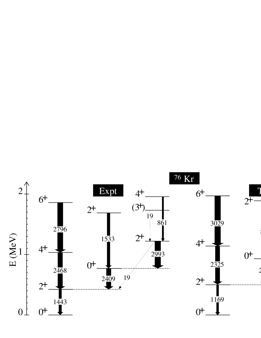
Figure 1: Experimental and theoretical spectra (MeV) and transition strengths ($e^{2}fm^{4}$) of ⁷⁶Kr showing the excitations that we examine in the present global study. The experimental spectrum, on the left, is from Ref. cl07 as well as from data repository for the $3^{+}$ and $4^{+}$ members of the $\gamma$ band brookhaven . Calculated values are those from Ref. cl07 .

The experimental spectrum is also shown in the figure, and one sees that excitation energies are reproduced very well. The calculated excitation energy of the first excited state, the $2^{+}_{1}$, is only 21% higher than experiment. The other states are proportionally even closer: the energies of the yrast $4^{+}_{1}$ and $6^{+}_{1}$ states are within 10% of the experimental values. Even the non-yrast excited state energies come out well. We shall later examine systematically the $0^{+}_{2},2^{+}_{2}$ and $2^{+}_{3}$ excitations; in ⁷⁶Kr  their predicted energies are all within 20% of experiment. For the transition strengths, the predicted $B(E2;2^{+}_{1}\rightarrow 0^{+}_{1})$ is within 20% of the experimental value and the higher transitions along the yrast ladder are within 10%.

The second excited state in the ⁷⁶Kr system is the $0^{+}_{2}$ level at 0.77 MeV. The calculated energy is 0.92 MeV, close enough to make a correspondence between the two states. Its mean deformation parameters are close to those of the ground state, suggesting a $\beta$-vibrational interpretation. The transition rate to the $2^{+}_{1}$ state is large and in very good agreement with experiment. The $2^{+}_{3}$ excitation corresponds in excitation energy fairly well to experimentally measured state. The $2^{+}_{3}$ wave function has a large probability $P(K=0)$, suggesting that it be placed with the $0^{+}_{2}$ level as member of the K = 0 excited structure. Its transition strength to the $0^{+}_{2}$ is large and in qualitative accord with experiment. Experiment and calculation for the spectroscopic quadrupole moment Q$(2^{+}_{3})$ are also in accord for both magnitude and sign. The sign is opposite to that for Q$(2^{+}_{1})$, nullifying any interpretation of the K = 0 excited structure as $\beta$-vibrational band and giving weight to the interpretation of shape coexistence between prolate and oblate band structures.

From the energetics, the $2^{+}_{2}$ level might be assigned at a two-phonon excitation of the ground state. The calculated $2^{+}_{2}$ wave function has a large probability for $K=2$ ($P(2)=0.77$), suggesting that this level instead is the bandhead of a $\gamma$-structure. However, the experimental data on the transition strengths between the $2^{+}_{2}$ and the $0^{+}_{2},2^{+}_{1}$ and $3^{+}_{1}$ states are very far from the theoretical predictions. Since transition strengths of $\gamma$-vibrations are very sensitive to $K$-band mixing, the disagreement of transition strengths does not rule out the $\gamma$-vibrational interpretation. For more discussions, see cl07 .

We finally mention the highest excitations, some of which will be beyond the scope of our global survey. There is good accord between theory and experiment for the energetics of the $6^{+}_{1}$ state as well as for those for the $3^{+}_{1}$ and $4^{+}_{2}$ levels which both form a quasi-$\gamma$ band structure on top of the $2^{+}_{2}$ state. The $6^{+}_{1}$ and $4^{+}_{2}$ states have strong transitions to the $4^{+}_{1}$ and $2^{+}_{2}$ states, respectively, in both theory and experiment.

To summarize, the CHFB+5DCH theory provides a very good description of low-lying excited states ⁷⁶Kr spectrum. While not all aspects are reproduced, many of the energies and relative transition strengths are given to good accuracy. The complex spectra of the Kr isotopes have often been discussed as a shape coexistence phenomenon, and the theory does rather well in describing these features as well as shape transitions in this region gi09 .

III.2 ¹⁵²Sm

The nucleus ¹⁵²Sm lies at the start of the deformed lanthanide region of the nuclear chart and is considered as landmark in the identification of first-order quantum phase transition between spherical and axially deformed nuclei ia98 ; li09 . Its experimental level scheme is shown in the left-hand panel of Fig. 2, taken from Ref. brookhaven and our calculated level scheme is in the right-hand panel. We first note that the yrast band is well reproduced. The $2^{+}_{1}$ excitation energy is within 2% of the experimental one, and the experimental ratio of the $4^{+}_{1}$ to the $2^{+}_{1}$ energies is $R_{42}=3.0$, slightly lower than the rigid axial rotor value 10/3. The 5DCH ratio is 3.0, reproducing the slight deviation from rigidity. The yrast spectrum is intermediate between that for harmonic vibrators and axial rotors, consistent with predictions from the X(5) model designed as analytic description of critical point structures in N $\simeq$ 90 isotones ia01 ; ca01 . For a review see ca07 .

Figure 2: Experimental and theoretical spectra (MeV) of ¹⁵²Sm. The experimental spectrum is based on Ref. brookhaven .

Table 1: Experimental and theoretical E2 transition strengths $B(E2;J_{i}\rightarrow J_{f})$ ($e^{2}fm^{4}$) of ¹⁵²Sm. From left to right : exp1 and exp2 are for $B(E2)$ experimental data from Ref.ku07 and za99 ; kl00 ; ca01 ; bi03 ; ca07 , respectively, and th are for 5DCH calculations.

$J^{\pi}_{i}$	$\rightarrow$	$J^{\pi}_{f}$	exp1	exp2	th
$6^{+}_{1}$		$4^{+}_{1}$	11795(347)	11805(241)	12042
$4^{+}_{1}$		$2^{+}_{1}$	10061(277)	10071(144)	10171
$2^{+}_{1}$		$0^{+}_{1}$	6938(144)	6938(144)	6671
$0^{+}_{2}$		$2^{+}_{1}$	1589(194)	1590(110)	2539
$2^{+}_{2}$		$0^{+}_{2}$	8048(763)	5156(1300)	4732
		$4^{+}_{1}$	867(97)	915(96)	768
		$2^{+}_{1}$	277(28)	265(24)	1066
		$0^{+}_{1}$	46(4)	43(5)	1.2
$4^{+}_{2}$		$2^{+}_{2}$	12488(2081)	9830(1831)	7505
		$6^{+}_{1}$	763(208)	193(96)	655
		$4^{+}_{1}$	291(55)	260(63)	977
		$2^{+}_{1}$	36(6)	48(9)	27
$2^{+}_{3}$		$0^{+}_{1}$	179(12)	174(8)	430
		$2^{+}_{1}$	451(28)	448(24)	77
		$4^{+}_{1}$	34(3)	38(2)	686
		$0^{+}_{2}$	2(0.2)	$<$2.4	1376
		$2^{+}_{2}$	604(42)	1301(193)	7382
$3^{+}_{1}$		$2^{+}_{1}$		337-819	479
		$4^{+}_{1}$		337-867	389
		$2^{+}_{2}$		$<$25	1974
		$2^{+}_{3}$		2987-38451	6627
$4^{+}_{3}$		$2^{+}_{1}$		28(8)	228
		$4^{+}_{1}$		265(77)	4384
		$6^{+}_{1}$		58(19)	663
		$2^{+}_{2}$		9(3)	140
		$4^{+}_{2}$		$<$1686	1209
		$2^{+}_{3}$		2409(723)	5045
		$3^{+}_{1}$		$<$12046	4384

We now come to the predictions for the $0^{+}_{2}$ excitation and the collective structure built upon it. The calculated deformation of that state is $\langle\beta\rangle=0.29$, almost the same as the ground state deformation, $\langle\beta\rangle=0.30$. This suggests an interpretation as a $\beta$-vibration. One expects that the fluctuation in $\beta$ would be larger in the vibrational excitation than in the ground state; in the harmonic limit, $<n|\beta^{2}|n>=(n+1/2)/B_{00}\,\omega$, giving a ratio of $\sqrt{3}$. In fact, the fluctuation in the calculated wave functions is larger for the excited state, by a factor 1.58. Thus, the theoretical wave function has the main characteristics to be a $\beta$-vibration.

Comparing experimental and calculated spectra, we first note that the calculated excitation energy of the $0^{+}_{2}$ state is quite a bit higher than observed experimentally, by nearly 40%. As we will see later, this is a common feature of the CHFB+5DCH theory as presently implemented. The experimental energy splitting between the $2^{+}_{2}$ and $0^{+}_{2}$ states is nearly identical to that of the ground state band, while the theoretical splitting is larger by 40%. This discrepancy is in keeping with that of the X(5) model ca07 . We conclude that the theory confirms in an approximate manner the existence of a band structure based on the $0^{+}_{2}$ excitation, but in detail deviates from the $\beta$-vibrational limit in the in-band energetics.

The CHFB+5DCH theory also predicts a $2^{+}_{3}$ excitation and collective structure upon it. This sequence is interpreted as a quasi $\gamma$-vibrational band, with head level energy slightly higher than that observed in this nucleus. Our calculated third $2^{+}$ state has the same average $\langle\beta\rangle$ deformation as the ground state, supporting a vibrational interpretation. If it were a true $\gamma$-vibration, it should have high probability for the $K=2$ component of the wave function. This probability is 0.64 compared with 0.002 and 0.35 for the $2^{+}_{1}$ and $2^{+}_{2}$ levels, respectively. Thus, the $2^{+}_{3}$ state has a qualitative character as a $\gamma$-vibration but this is diluted by other components. This is to be expected for a transitional nucleus such as ¹⁵²Sm.

Important indicators for structure properties are the strengths for intra- and inter-band E2 reduced transition probabilities. $B(E2;I_{i}\rightarrow I_{f})$’s measured by the Georgia Tech. and Yale collaborations are shown in Table 1 together with CHFB+5DCH calculations. As the two sets of experimental data display differences, comparison between B(E2) predictions and measurements necessarily has a global character. The figure of merit of our theory for ¹⁵²Sm is as follows : i) the intraband transition strengths have right order of magnitude, especially for the ground state band, ii) the transition between $\gamma$ and ground state as well as between the $\gamma$ and $\beta$ bands are too collective, and iii) the $\beta$ to ground state band transitions display a mixed character. The theory for the $0^{+}_{2}\rightarrow 2^{+}_{1}$ transition strength is about 60% too high. Nevertheless we conclude that the $0^{+}_{2}$ excitation is a $\beta$-vibration in ¹⁵²Sm.

Our present conclusion is that the structure of the ground state, $\beta$-, and quasi-$\gamma$ bands is globally as the 5DCH theory predicts, but there are probably other components in the wave functions, such as 2qp excitations and pairing isomerism Kulp05 that may have an important large effect on the out-of-band transitions. More accurate B(E2) measurements that are underway ca09 will be a valuable asset for making definite statements on the predictive character of present 5DCH calculations and for disclosing which degrees of freedom might be missing in the structure models including the 5DCH one.

IV Ground state properties

IV.1 Nuclear shapes

We begin by displaying in Fig.3 the set of nuclei that we have calculated and included in our tables. This comprised all even-even nuclei that are stable with respect to two-particle emission, and that have positive correlation energies in the CHFB+5DCH theory. Among the $Z>96$ nuclei, some ones close to the proton drip line have been removed from the chart as their inner potential barriers are too low for inhibiting fission decay. For now, we remark that the two-particle stability is almost completely determined by the HFB energies. The correlation energy $E_{corr}$ contribution (see Eq.(15)) only changes it for a few nuclei on the borders. The next general remark is that the criterion of positive correlation energy affects only nuclei at magic numbers. These are visible as the absence of colored circles along some of the magic number dotted lines.

In the figure, the color coding shows the deformation $\beta$ of the ground state, with a $\pm$ sign according to the value of $\gamma$. For the HFB ground states, shown in the left-hand panel, one sees the familiar landscape of nuclear shapes, with nuclei near magic numbers having small or vanishing deformation (dark and medium green), and two large deformed regions located at the lanthanides and actinides. Additional regions of deformation are centered at nuclei with $(Z,N)=(12,12),(38,40),(40,60)$, and $(60,80)$, the heavy nuclei with $N\sim 150$, and the superheavy nuclei with $N>190$. It is also apparent that single magic numbers do not enforce sphericity. For example, the Sn isotopes are spherical in the region below $N\sim 82$, become deformed for neutron numbers in the range $N\sim 100-112$, and get back to spherical shapes beyond $N\sim 114$ up to the neutron drip-line.

The right-hand panel shows the expectation value $\langle\beta\rangle$ for the CHFB+5DCH calculation, with the sign determined by the expectation value of $cos(3\langle\gamma\rangle)$.

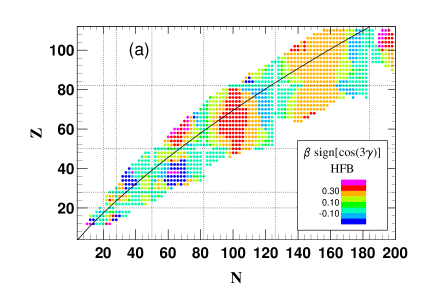
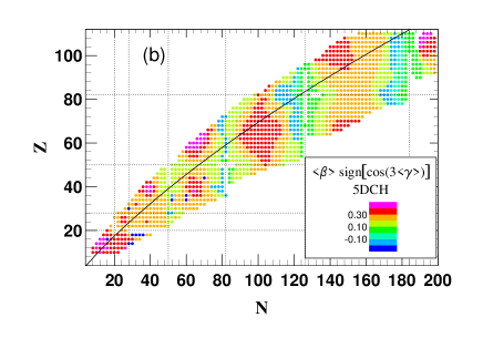
Figure 3: (Color online) Chart of nuclides showing ground state deformations. Panel (a): HFB minimum; panel (b): expectation value in the 5DCH ground state. The black curve shows the beta-stability line.

The 5DCH wave functions have larger deformations on average with fewer nuclei near sphericity. To better see how the 5DCH changes the deformation properties, we show in Fig. 4 histograms of the distributions of $\beta$ and $\gamma$. The result for the distribution of $\beta$ in the HFB theory is shown on the upper left-hand panel. Among the 1712  nuclei in the calculated data set, roughly 30% are spherical. The rest has a broad distribution of deformations peaking at $\beta\approx 0.25$. Except for the very heaviest nuclei, the largest deformation of the survey was found for the nucleus ²⁴Mg, with $\beta=0.54$. The lower left-hand panel shows the corresponding distribution of $\gamma$. For this plot, we restricted the nuclei to those with $\beta>0.1$, because $\gamma$ is ill-defined in spherical nuclei. One sees that the great majority of the nuclei are prolate and axially symmetric, i.e. $\gamma\simeq 0$. There is also a small peak for oblate shapes, $\gamma=60^{\circ}$, comprising about 15% of the deformed nuclei. The paucity of oblate deformations compared to prolate is well-known in mean-field calculations ta96 ; st09 . However, it should be mentioned again that our calculated nuclei include only those having positive correlation energies. The others are all near magic numbers and are likely to be spherical. Turning to the 5DCH $\langle\beta\rangle$ distributions shown in the upper right-hand panel of Fig. 4, we see essentially all the nuclei become deformed, with deformation broadly distributed in the range $0.05\leq\langle\beta\rangle\leq 0.4$. The corresponding distribution of axial asymmetries $\langle\gamma\rangle$ in the lower left-hand panel shows that axial symmetry disappears in the 5DCH wave functions, with average asymmetries going up to $30^{\circ}$.

Additional information about shape fluctuations is provided by the variances in the deformation parameters, Eq. (16). In principle, the value $\gamma=30^{\circ}$ could arise from a potential energy surface that is very soft in the $\gamma$ coordinate or from one that has a strong triaxial minimum. Fig. 5 shows the distribution of rigidity measures $\langle\beta\rangle/\delta\beta$ and $\langle\gamma\rangle/\delta\gamma$ for $\beta$ and $\gamma$, respectively. The $\beta$-rigidity goes to very high values, $\langle\beta\rangle/\delta\beta\sim 10$ in the deformed actinides. We will find that such high values are present when the nucleus has a well-developed rotational spectrum. On the other hand, the $\gamma$-rigidity is much smaller and is never more than $\sim 3$. Without a clear peaking at very large values, it will be problematic to characterize the nuclei in terms of the simple models for triaxial shapes.

Figure 4: Distributions of $\beta$ and $\gamma$ in ground states. Panels a) and c): distribution of the HFB minima. Several nuclei at $Z\sim 108$ have minima at $\beta\sim 0.75$ and are not shown. Panels b) and d): distributions of $\langle\beta\rangle$ and $\langle\gamma\rangle$ in the CHFB+5DCH ground state. The distribution of $\gamma$ in the lower left-hand figure includes only nuclei with nonspherical minima. The histogram on lower right-hand includes nuclei having spherical HFB minima as well. Units for $\gamma$ and $\langle\gamma\rangle$ are degrees.

Figure 5: Distribution of rigidity parameters, namely $\langle\beta\rangle/\delta\beta$ in panel a) and $\langle\gamma\rangle/\delta\gamma$ in panel b).

IV.2 Radii

We now examine the predicted charge radii, which we compare with the tabulated experimental data from Refs. an04 ; fix . The mean square charge radii $r_{c}^{2}$ are calculated as ne70

$$r_{c}^{2}={1\over Z}\int r^{2}d^{3}r\,n_{p}(r)+r_{p}^{2}+{N\over Z}r_{n}^{2}-r_{cm}^{2},$$ (17)

where $n_{p}(r)$ is the point-proton density, and $r_{p}^{2}=0.63$ fm² and $r_{n}^{2}=-0.12$ fm² are the rms proton and neutron charge radii, respectively. The center-of-mass correction is computed as $r_{cm}^{2}=3\hbar^{2}/2m\omega A$ fm² (see Eq.(4.3) in Ref.ne70 ), with $\omega=1.85+35.5/A^{1/3}$ MeV. We show in Fig. 6 the comparison of calculated and experimental charge radii, plotted as the relative error

$$\epsilon=r_{c}^{th}/r_{c}^{exp}-1.$$ (18)

The upper and lower panels show the HFB and the CHFB+5DCH results, respectively, with lines connecting nuclei in isotopic chains. We see that the theory is remarkably accurate at the HFB level, and the CHFB+5DCH hardly changes the predictions. Among the heaviest nuclei, we find that the U isotopes are reproduced very well. The theory seems to be high for the Cm isotopes, but it should be noted that these radii were based on systematics in the absence of any direct measurement angeli .

Nucleus-to-nucleus variations in radii can be attributed to deformation changesotten as well as other nuclear structure effects ta93 ; re95 ; sh95 . The effects of deformation can be easily seen in individual isotopic chains. An example is the Sr isotopic chain, shown in Fig. 7. Experimentally, one sees a slight decrease in the radius from $N=40$ to the $N=50$ magic number, followed by a much steeper increase in radii as more neutrons are added. The HFB minima are spherical below $N=50$ and deformations increase to very large values at the heaviest isotopes in the figure. That results in almost monotone increase in radius from the lightest to the heaviest isotopes.

Turning to the CHFB+5DCH results, we find that the main effect is in the lighter nuclei, and it is to increase the charge radius. This is to be expected, since deformations increase the radius and the average deformations are systematically larger in the CHFB+5DCH. The largest increase, by 4%, is in the nucleus ³⁰Si. Here the HFB minimum is spherical, while the CHFB+5DCH ground state has a mean deformation $\langle\beta\rangle$ = 0.48. Returning to the Sr isotopic chain, the correlations associated with the CHFB+5DCH bring the theory in very good overall agreement with data. This comes about from two effects. In the very light isotopes, the CHFB+5DCH predicts large deformations instead of the spherical shape of the HFB minimum, increasing the radii. On the other end of the isotopic chain the nuclei are also deformed, but the average deformation in the CHFB+5DCH wave functions ($\langle\beta\rangle\sim 0.3-0.35$) is less than in the HFB minima ($\beta\sim 0.45)$.

Table 2 shows the performance of the theory, using as a quantitative measure the rms dispersion $\sigma$ about the mean $\bar{\epsilon}$, $\sigma=\langle(\epsilon-\bar{\epsilon})^{2}\rangle^{1/2}$. Both HFB and the CHFB+5DCH treatments, suitably renormalized, are accurate to 0.6%. For a comparison, the 2-parameter “Finite surface” model an04 taking $r_{c}=r_{0}A^{1/3}+r_{1}A^{-1/3}$ fm is shown in the third row of the Table. Here the error is about twice as large.

Figure 6: Charge radii. Plotted are the relative errors, Eq. (18), with isotopic chains connected by lines. Panels a) and b) show the results of the HFB and the CHFB+5DCH theories, respectively. Experimental data is from Refs. an04 ; bu00 ; ca02 (see fix ) and includes 313 nuclei.

Figure 7: Charge radii $r_{c}$ of Sr isotopes. Experimental: circles joined by solid line; HFB: triangles joined by dot-dashed line; CHFB+5DCH: squares joined by dotted line.

Table 2: Comparison of calculated charge radii with experiment: $\bar{\epsilon}$ is the mean of $\epsilon$ (see Eq. (18)); $\sigma$ is its rms dispersion about the average. 313 nuclear radii were included in the comparison as in Fig. 6. In the column “HFB (new)” we use the modern value $r_{p}=0.875$ fm for the proton charge radius PDG .

Theory	$\bar{\epsilon}$	$\sigma$
HFB	0.001	0.006
HFB (new)	0.005	0.007
CHFB+5DCH	0.006	0.007
Finite Surface	0.0000	0.012

IV.3 Correlation energies

A key observable that theory should describe is nuclear masses or equivalently their binding energies. We shall consider the binding energy to be composed of two terms, the binding energy of the mean-field minimum calculated in an unconstrained (with respect to shape) HFB calculation, and the correlation energy associated with the spread of the wave function over the quadrupole shape degrees of freedom. For an orientation, we show in Fig. 8 these two contributions and their sum, displayed as difference between experimental Au03 and theoretical energies (i.e. residuals). One can see that the shell effects at $N=82$ and 126 are too large in the HFB theory, and the correlation energies vary in a way to reduce the shell effects to a level closer to that needed.

Figure 8: Panel a): residuals of the HFB binding energies with respect to experiment, plotted as a function of neutron number with nuclei of the same $Z$ connected by lines. Panel b): Correlation energy, Eq. (15). Panel c): residuals including correlation energies. Experimental data is from Ref. Au03 .

The overall performance of the theory with respect to masses depends extremely sensitively on the parameters of the functional, and any useful theoretical mass table requires that the force parameters be refitted. This has been recently carried out for the Gogny D1N and D1M parametrizations hilaire . However, in the present study we will keep the original D1S interaction and evaluate the performance with respect to differential quantities, which are much less sensitive to the precise parameters of the interaction. The first quantity we examine is the two-nucleon separation energy defined as

$$\begin{array}[]{lr}S_{2n}(N,Z)=E(N-2,Z)-E(N,Z),&{\rm 2\-n~{}separation~{}energy},\\ S_{2p}(N,Z)=E(N,Z-2)-E(N,Z),&{\rm 2\-p~{}separation~{}energy.}\\ \end{array}$$ (19)

In the left- and right-hand panels of Fig.9 we show the two-nucleon separation energies $S_{2n}$ and $S_{2p}$ for the HFB and the CHFB+5DCH calculations, presenting the calculations in a similar way as was done in Ref. be08 . The shell gaps are quite obvious, and one can see that they are reduced in the CHFB+5DCH theory. The available experimental data is shown on the bottom panels. One can see that the shell gap varies with the number of nucleons of opposite isospin. In particular, it is observed in the right-hand panel for the proton separation energies that the $Z=50$ and $Z=82$ shell gaps disappear at high neutron excess. As mentioned earlier, the ground states become deformed in these neutron-rich nuclei.

In the left-hand panel for $S_{2n}$ one also sees a gradual opening of the $N=162$ spherical shell gap for proton numbers $Z>96$. This gap 2.5 MeV wide for Z = 110 should increase stability of superheavy elements (SHEs). Our predictions are consistent with those based on calculated shell correction energies smol95 , and with the observation of a minimum in alpha-decay energies of SHEs at $N=162$ (for a review see oga07 ). Impact of this neutron gap on calculated $S_{2p}$ values is also seen for $N\simeq 162$ in the right-hand panel. Finally we note that Interacting Boson Model calculations are also supporting evidence for a neutron spherical gap in close vicinity of $N=162$ bre94 .

Another phenomenon is the enhancement of the gap near doubly magic nuclei. This phenomenon, called “mutually enhanced magicity” Lu03 , is reproduced much better by the CHFB+5DCH theory than by the HFB. The best example is the $Z=82$ gap of the $S_{2p}$ systematics in the bottom right-hand panel, which becomes larger near $N=126$. Unfortunately, the Gaussian Overlap Approximation does not permit us to calculate the doubly magic nuclei.

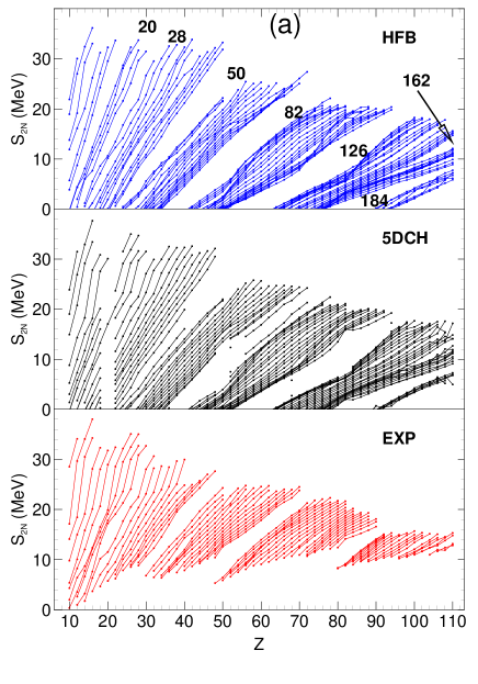
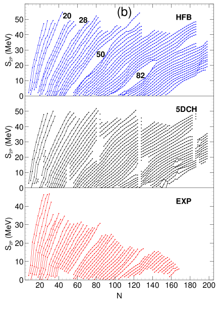
Figure 9: (Color online) Panel (a) : two-neutron separation energies; panel (b): two-proton separation energies. The three rows show the HFB theory, the CHFB+5DCH theory, and experiment, respectively. Experimental data is from Ref. Au03 .

In Table 3 we show the rms residuals of the calculated separation energies with respect to experiment. The experimental data is from Ref. Au03 , including only nuclei whose binding energies are given with experimental error of less than 200 keV. As already mentioned, our theory only includes nuclei whose correlation energy is positive. This excludes only about 10% of the nuclei in the experimental data set. The number of nuclei in the comparison is given on the first line of the table. The first comparison, with the HFB energies, shows rms residuals of slightly less than 1 MeV for both separation energies and gaps. The performance here is slightly better than was found in the survey based on the Skyrme energy functional Sly4, reported in Ref.Ben06 . The bottom line of the table shows the energies of the full CHFB+5DCH theory, i.e. with the correlation energy included. The improvement is about 25%. This is surprisingly comparable to the results found in Ref. Ben06 , despite that correlation energy was calculated in a completely different way.

Table 3: 2-nucleon separation energies and gaps. Sizes of the compared data sets are given on the first line. Rms residuals with respect to experiment are given on the third and fourth lines, for the HFB and CHFB+5DCH theories, respectively. Energies are in MeV.

		$S_{2n}$	$S_{2p}$	$\delta_{2n}$	$\delta_{2p}$
Size	theory	455	433	396	358
	exp.	492	467	444	392
Theory	HFB	1.00	0.91	1.06	0.98
	CHFB+5DCH	0.72	0.71	0.68	0.61

We also carried out the statistics on the two-nucleon gaps. This quantity is defined by the next higher order difference,

$$\begin{array}[]{lr}\delta_{2n}(N,Z)=S_{2n}(N+2,Z)-S_{2n}(N,Z),&{\rm 2\-n~{}gap},\\ \delta_{2p}(N,Z)=S_{2p}(N,Z+2)-S_{2p}(N,Z),&{\rm 2\-p~{}gap}.\\ \end{array}$$ (20)

As a particular example, there has been much discussion of evolution of the $Z=28$ gap for high neutron numbers. We find that the CHFB+5DCH energies are below the HFB values, thus weakening any shell effect at $Z=28$. There is a peaking at $N=28$ that could be attributed to “mutually enhanced magicity” or to an $Z=N$ symmetry effect, the “Wigner energy”. Experimentally, there is a slight peaking in the gap at $N=40$, but we find that it is smooth in the CHFB+5DCH theory.

The overall statistics for the performance of the theories with respect to two-nucleon gaps are also shown in Table 3. The results are somewhat better than those for the separation energies.

V Yrast spectrum

In this section we report the predictions for the lowest excitations of angular momentum $J=2,4$ and $6$. For the quantitative measure of the global performance of the theory, we will use the same figures of merit as in Ref. be07 . Because the quantities span a large range values, we examine the statistics of the logarithmic ratio of theory to experiment, namely

$$R_{x}=\log(x_{th}/x_{exp}),$$ (21)

for a quantity $x$. We present its average over the data set $\bar{R}_{x}$ as well as the dispersion about the average,

$$\sigma_{x}\equiv\langle(R_{x}-\bar{R}_{x})^{2}\rangle^{1/2}.$$ (22)

The results for the properties we can compare with tabulated experimental data are discussed individually below and in Sec. VI, and are summarized in Table 4 in Sec. VII.

V.1 The first $2^{+}$ excitation

The first physical property we examine is the fraction of the energy-weighted sum rule (EWSR) contained in the $2^{+}_{1}$ excitation. That quantity is governed more by the inertial and mass properties of the CHFB+5DCH than by the topology of the potential energy surface. The sum rule fraction is often expressed with respect to Lane’s isoscalar sum rule  Lane

$$S(I)=\sum_{i}E(2^{+}_{i})B(E2;0^{+}_{1}\rightarrow 2^{+}_{i})={25\over 4\pi}(\frac{\hbar^{2}}{m})A\langle r^{2}\rangle,$$ (23)

where $m$ is the nucleon mass and $\langle r^{2}\rangle$ is the mean square mass radius. It is also common to make the approximation $\langle r^{2}\rangle=1.2^{2}A^{2/3}$ fm² ra01 but we shall rather use our calculated mass radius. The charged part of the isoscalar sum rule is derived from $S(I)$ assuming that the charge current and mass current are proportional ra01

$$S(II)=S(I)(\frac{Z}{A})^{2}.$$ (24)

The fraction s(X) of the sum rules carried by the $2^{+}_{1}$ excitations is calculated as

$$s(X)=E(2^{+}_{1})B(E2;0^{+}_{1}\rightarrow 2^{+}_{1})/e^{2}S(X),\,\,\,{\rm with}\,\,\,X=I,II.$$ (25)

Histograms of s(I) and s(II) are shown on the left-hand panel of Fig. 10. Individually, the excitation energies and transition strengths vary over several orders of magnitude. But their product scaled by $s(X)$ compresses the rms variation down to about a factor of 2. This may be seen in the histograms of $s(I)$ and $s(II)$ shown in the left-hand panel of Fig. 10. The fraction of strength in each sum rule is about 1.5$\%$ for $S(I)$ and 10% for $S(II)$. As well known, most of the strength is carried by the giant quadrupole resonance. One can also see from the histograms that the scaling with $S(II)$ produces more compressed distribution than scaling with $S(I)$. A scatter plot of the theory versus the experimental values of $S\equiv E(2^{+}_{1})B(E2;0^{+}_{1}\rightarrow 2^{+}_{1})$ is shown on the right-hand panel of Fig. 10. There is a concentration of points on the diagonal that show very good agreement; these mostly correspond to strongly deformed nuclei. Overall, the theory somewhat overestimates the fraction of the EWSR carried by the $2^{+}_{1}$ state.

Figure 10: Panel a): distribution of sum rule fraction $s(X)$, Eq. (25), in the CHFB+5DCH theory, for the 1609 calculated nuclei. Solid and dashed lines show the fraction of the S(I) and S(II) sum rules, respectively. Panel b): calculated $S\equiv E(2^{+}_{1})B(E2;0^{+}_{1}\rightarrow 2^{+}_{1})$ versus experimental, for 311 nuclei. Experimental data are from Refs. ra01 ; sh94 . S values are in MeV-$e^{2}b^{2}$ units.

We now turn to the comparison of excitation energies and transition strengths with experiment. The results were reported already in Ref. be07 , but we since discovered that the code we had been using to solve the 5DCH did not have the desired precision for smallest excitation energies. In the present work we report recalculated energies using a more accurate code described in Refs. li82 ; Li99 . The comparison of experiment ra01 ; sh94 and the calculation is shown in the left-hand panel of Fig. 11. The points at the lower left correspond to the deformed lanthanides and actinides, and one sees that the theory does very well there.

Figure 11: Panel a): theoretical $2^{+}_{1}$ excitation energies of 537 even-even nuclei as a function of their experimental values. Panel b): theoretical $B(E2;0^{+}_{1}\rightarrow 2^{+}_{1})$ transition strengths of 320 even-even nuclei as a function of their experimental values. Several cases showing deviations are labeled by the nucleus. Experimental data is from Refs. ra01 ; sh94 .

Right-hand panel of Fig. 11 shows a similar comparison for the $B(E2;0^{+}_{1}\rightarrow 2^{+}_{1})$ transition strength. The points on the upper right side of the figure correspond to the very deformed actinide nuclei. Again, the theory is seen to be remarkably accurate under the conditions of a large static deformation. The global performance figures of merit for the $2^{+}_{1}$ energy and the $B(E2;0^{+}_{1}\rightarrow 2^{+}_{1})$ strength are given on the first two lines of Table 4 posted in Sec. VII.

V.2 The first $4^{+}$ excitation and $R_{42}$

An important signature of the character of the excitation spectrum is the relationship of the lowest $4^{+}$ excitation and the $2^{+}_{1}$ below it. A very useful indicator is the ratio of the two excitation energies $E(J^{\pi}_{n})$,

$$R_{42}={E(4^{+}_{1})\over E(2^{+}_{1})}.$$ (26)

The $R_{42}$ indicator has been much used, particularly in discussing complex spectra. The value $R_{42}=10/3$ is characteristic of an axial rotor, $R_{42}=2$ of a vibrator, and $R_{42}=5/2$ of a $\gamma$-unstable rotor or the $O(6)$ algebraic model ca00 . In Fig. 12 we display histograms of the experimental and theoretical ratios side by side. One sees a very narrow peak at 10/3, showing that one can make a nearly unambiguous assignment of axial rotors. In the algebraic models the three simple limits mentioned above represent extremes in the parameter space of the models, and it is interesting to see which ones are favored in the global systematics. While the axial rotor is clearly special, neither the harmonic vibrator nor the $\gamma$-unstable rotor shows a corresponding accumulation in the experimental data. The CHFB+5DCH theory, on the other hand, does show a second peak just below the $\gamma$-unstable value, $R_{42}=5/2$.

Figure 12: Panel a): histogram of experimental $R_{42}$ ratios, Eq. (26), for 501 even-even nuclei, with data from Ref. brookhaven . Panel b): histogram of calculated $R_{42}$ ratios for 1609 even-even nuclei calculated in the CHFB+5DCH theory.

It is interesting to see how well the physical structure indicator $R_{42}$ correlates with the intrinsic shape properties of the CHFB+5DCH wave functions. Let us first examine the relationship between $R_{42}$ and mean deformation $\langle\beta\rangle$. This is shown in the left-hand panel of Fig.13. One can see that the value of $\langle\beta\rangle$ by itself does not determine whether the yrast spectrum has a rotational character. The $R_{42}$ has the rotational value for $\langle\beta\rangle$ in the range $0.2-0.45$, but nuclei with nonrotational spectra are common with $\langle\beta\rangle$ values up to 0.3. In fact the highest value of $\langle\beta\rangle$ in our calculations is found for a nucleus (²⁶Mg) for which $R_{42}=2.4$, both theoretically and experimentally. Evidently, what is needed as well to determine the rotational properties is a measure of the rigidity of the shape. For that purpose, we use the $\beta$-softness parameter, $r_{\beta}=\delta\beta/\langle\beta\rangle$. The $R_{42}$ values are plotted with respect to $r_{\beta}$ in the right-hand panel of Fig. 13. As may be seen from the figure, this provides a much better separation between the rotational and nonrotational spectra. Effectively, the $\beta$-softness parameter should be less than 0.2 for a rotational spectrum.

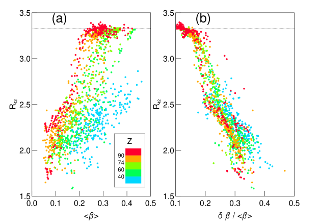
Figure 13: (Color online) The ratio $R_{42}$ as a function of the mean deformation $\langle\beta\rangle$ (panel (a)) and the $\beta$-softness parameter $\delta\beta/\langle\beta\rangle$ (panel (b)) for the calculated nuclei in their ground states. Dotted lines show the rigid rotor value $R_{42}=10/3$.

We turn to the performance of the theory of the $4^{+}_{1}$ level, comparing energies to experimental data. Of the 484 nuclei with tabulated experimental energies brookhaven , 480 meet the criteria to be included in our theoretical data base. Left-hand panel of Fig. 14 shows the comparison of the theory to experiment as a scatter plot for $R_{42}$. For most nuclei the $R_{42}$ values in both measurements and calculations fall between $R_{42}$ = 2 and $R_{42}$ = 10/3 limits of the vibrational and rotational models, respectively. Values of $R_{42}$ less than one are certainly possible when the spectrum is dominated by two-quasiparticle excitations, which is common near magic numbers.

Figure 14: Panel a): $R_{42}$ comparison of theory and experiment for 480 nuclei. Arrows indicate the rigid rotor value $R_{42}=10/3$. Experimental data is from Ref. brookhaven . Panel b): distribution of $R_{42}(B)$ for CHFB+5DCH wave functions of 1693 nuclei.

Statistical performance for the data set is given in Table 4. The average value of the ratio $R_{42}$ comes out very well, only 3% higher than the measured average. The dispersion about the mean is also quite good, better than the predictions for the absolute energies of the $2^{+}_{1}$ excitations.

In the subsections below, we will analyze the properties of other excitations with respect to the rotational character of the ground state. Since the $R_{42}$ measure is very clear, we shall make much use of it to examine the connections.

It is of interest to examine the transition strengths $B(E2;4^{+}_{1}\rightarrow 2^{+}_{1})$, even in the absence of a critical review and evaluated tabulation of the experimental data. To interpret this quantity we take the ratio to the $2^{+}_{1}\rightarrow 0^{+}_{1}$ transition, defining $R_{42}(B)$ as

$$R_{42}(B)=\frac{B(E2;4^{+}_{1}\rightarrow 2^{+}_{1})}{B(E2;2^{+}_{1}\rightarrow 0^{+}_{1})}.$$

Two anchor points to interpret $R_{42}(B)$ are the axial rotor model for which $R_{42}(B)=10/7$, and the harmonic vibrator model for which $R_{42}(B)=2$. The distribution of calculated values is shown as a histogram in the right-hand panel of Fig. 14. There is a peak at the axial rotor value, but no peak at the vibrator value or anywhere else. The calculated $R_{42}(B)$ range from 1.43 for the nucleus ²⁴⁰Cm to 5.7 for the nucleus ¹⁸⁰Pb. There are no calculated nuclei with $R_{42}(B)$ smaller than the axial rotor value.

V.3 The first $6^{+}$ excitation

The last excitation we shall examine in the yrast spectrum is the $6^{+}_{1}$ level. If the $0^{+}_{1},2^{+}_{1}$, and $4^{+}_{1}$ levels form a band with energies close to the axial rotor limit, the $6^{+}_{1}$ state is also part of the band in the vast majority of cases. Deviations of its energy from the rotational limit can also be extrapolated from the $R_{42}$ values using the Mallman systematics ma59 ; bu08 , namely the empirical correlation of the ratios $R_{62}=E(6^{+}_{1})/E(2^{+}_{1})$ and $R_{42}$. The correlation associated with the CHFB+5DCH energies is shown in Fig. 15, left-hand panel, based on theoretical energies from 1609   nuclei. The scatter plot follows a line from about $(R_{42},R_{62})=(1.5,2.0)$ to the value $(10/3,7)$ corresponding to the rotational limit. The plot shows an accumulation of points at the axial rotor limit, as well as a somewhat broader peaking near $(2.3,3.7)$. For orientation, the positions of the $\gamma$-unstable limit and the harmonic vibrator limit are for $(5/2,4.5)$ and $(2,2)$, respectively. The experimental scatter plot of $R_{62}$ vs. $R_{42}$ is shown in the right-hand panel of Fig. 15. It shows data for 458 nuclei, obtained from the Brookhaven database brookhaven . We also show in the middle panel the calculated nuclei corresponding to the experimentally known ones. The experimental points form a line very much like the one seen in the theory plot. The correlation is also very narrow for the upper half of the line, but it becomes broader at lower values of $R_{42}$ and $R_{62}$. The experimental plot extends to lower values than we find in the theory. One possible explanation is the neglect of two-quasiparticle configurations in the theoretical wave functions. Such configurations can produce high angular momentum at relatively little energy cost, and therefore can give values of $R_{42}$ and $R_{62}$ close to 1. Also, the nuclei with such low $R_{62}$ values may have failed our criteria to keep in the theoretical database.

Figure 15: Ratios of yrast excitation energies, $R_{62}$, as a function of $R_{42}$. Panel (a): CHFB+5DCH theory for 1609 nuclei. Panel (c): experimental ratios for 456 nuclei, with data from Ref. brookhaven . Panel (b): theoretical values for the nuclei shown in the right-hand panel.

The global figures of merit of the observable $R_{62}$ are reported in Table 4. The reliability of the theory is quite high, although it does not do as well as for the lower 2⁺ and 4⁺ yrast excitations.

VI Non-yrast excitations

This section will examine in some detail the physical properties of $0^{+}_{2}$ and $2^{+}_{2}$ excited states but is also concerned with their possible role as head levels of collective bands, traditionally referred to as $\beta$- and $\gamma$-vibrational bands, respectively. In order to do this we will also need to consider the $2^{+}_{3}$ excitation, which can very often be considered as part of a $K=0$ excited band. The specific indicators we will examine in this context are the excitation energy with respect to band head, the in-band transition rate compared to that for the ground state band, and the relative out-of-band transition matrix elements. Unfortunately, the data tabulations do not exist to make a systematic comparison to experiment. However, the band character has been much discussed in the rare-earth region, and we can compare some out-of-band rates there. As the $2^{+}_{3}$ levels are almost systematically members of the excited K = 0 bands, an alternative to $\beta$-vibrational band interpretation is suggested, namely that of coexisting band structure inside nuclei. A detailed discussion of the $\gamma$-degree of freedom and associated collective band excitations is deferred to a later publication.

VI.1 The $2^{+}_{2}$ excitation

The lowest non-yrast excitation typically has $J=2$, and it is often interpreted in the collective model as a shape excitation in the $\gamma$ degree of freedom. A theoretical indicator for that character is the $K$-content of the wave function. This is shown visually in Fig. 16 indicating the probability $P(K)$ by the coloring of the nuclides. Apart from nuclei close to magic numbers, the vast majority of second $2^{+}$ states have $P(K=2)>0.75$ and can be considered as $\gamma$-vibrations. In the upper right corner of Fig. 16 is a domain without coloring. In this narrow mass region the inner potential barrier is not high enough to sustain excited states, and the nuclei go to fission. For a more quantitative view of the $K$ distributions we show them by histograms in Fig. 17 for the second and third $J=2$ states in the spectrum. For the $2^{+}_{2}$ state (left-hand panel), there is a sharp peak close to $P(K=2)=1$, together with a broader distribution of lower probabilities.

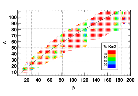
Figure 16: (Color online) Chart of the computed nuclei showing the probability of $K=2$ component in the wave function of the $2^{+}_{2}$ levels. The $2^{+}_{2}$ states with more than 75 $\%$ of $K=2$ components in wave functions are considered as $\gamma$-vibrations. The black curve shows the beta-stability line.

Figure 17: Probability of $K=2$ component in the wave functions of the second (panel a) and third (panel b) excited $2^{+}$ states.

For the most part, the nuclei within the sharp peak have $R_{42}$ close to the axial rotor value. Thus, for these nuclei we have a clear identification of the $2^{+}_{2}$ level as a $\gamma$-excitation.

The plot for the $2^{+}_{3}$ state in the right hand panel, shows that this level may be viewed as a $\beta$-excitation in many nuclei. Here the strong peak is at $P(K=2)=0$. Interestingly, there are a few nuclei for which the roles of the second and third state are reversed, as can be seen in Fig 16. It happens that our example ¹⁵²Sm in Sec. III is of this kind. In the discussion below, we will designate the second or third $2^{+}$ state with the larger $P(K=2)$ the $2^{+}_{\gamma}$ level, if $P(K=2)>0.75$ for all nuclei with $R_{42}\geq 2.3$ even though we know that $\gamma-$vibration is a designation specific to well deformed nuclei.

The systematics of the 5DCH $2^{+}_{\gamma}$ energies are shown in Fig. 18 (open circles) as a function of neutron number. The distribution of excitation energies displays sharp structures with maxima near N$\geq$ 50 magic numbers, for which $R_{42}<2.3$. Minima are found, as expected, half way between major closed shells and they reach very low values ($E_{x}\simeq 200$ keV) in heavy nuclei with Z$\geq$ 98.

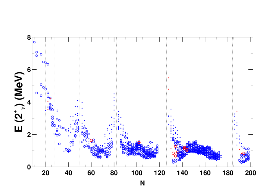
Figure 18: (Color online) Excitation energy of the CHFB+5DCH $2^{+}$ level with $P(K=2)\geq 0.75$ as a function of neutron number $N$. Open symbols in blue and red colors indicate the $2^{+}_{2}$ and the $2^{+}_{3}$ levels for nuclei with $R_{42}\geq 2.3$, respectively. These levels are defined as $2^{+}_{\gamma}$ excitations. Dots are for nuclei with $R_{42}<2.3$.

The performance of the CHFB+5DCH on the energies of the $2^{+}_{2}$ levels is shown in Fig. 19 through comparing the calculations to the evaluated data for 354 nuclei brookhaven .

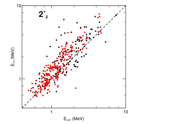
Figure 19: (Color online) Excitation energy of the second $J=2$ excitation, comparing 352 nuclei. Experimental data is from Ref. brookhaven . The $2^{+}_{\gamma}$ levels are marked with red color.

The theory clearly reproduces the variation of the experimental energies, which range over more than an order of magnitude. The colored symbols in this figure are for $2^{+}_{2}$ states identified as $2^{+}_{\gamma}$ levels in the CHFB+5DCH calculations. On average the theoretical energies are somewhat high. The figures of merit, given in Table 4, show that the theoretical energies average about 25% higher than the experimental ones. Interestingly, the variance $\sigma$ is smaller than that for the $2^{+}_{1}$ excitations.

VI.2 The $0^{+}_{2}$ excitation

In the framework of the CHFB+5DCH theory, the $0^{+}_{2}$ excitation can arise in several ways: as a $\beta$-vibration, as a coexisting state of very different shape, or something in between. To be a $\beta$-vibration, the excitation should have nearly the same $\langle\beta\rangle$ as the ground state, but a larger dispersion $\delta\beta$. The excitation in this limit is very dependent on the calculated mass parameters for the $\beta$ degree of freedom, which have been calculated using the Inglis-Belyaev formula. This treatment has known deficiencies and we expect that the predicted excitation energies would be somewhat lower if the Thouless-Valatin prescription were used. The other likely structure for the $0^{+}_{2}$ excitation arises from the coexistence of vastly different deformation at nearly the same energy. The latter mechanism is prominent in light doubly-magic nuclei be03 ; be03a and also in the actinides where the superdeformations occur at low excitation De06 ; kr92 ; ta98 . A phenomenological signature of coexistence would be a low excitation energy. In fact there are a number of known nuclei for which the $0^{+}_{2}$ level is the first excited state, but we do not find such a low excitation energy in our calculations. However this observation does not at all mean that the present theory is not able to provide reliable predictions for nuclei where shape coexistence and shape transition are present and characterized by many measurements. Such features are well described by our theory for the neutron-deficient Kr isotopes cl07 ; gir09 . That the present theory does not predict $0^{+}_{2}$ state as first excited state in a nucleus obviously means that degrees of freedom other than collective quadrupole ones are at play and cannot be ignored.

The theoretical and experimental excitation energies of the $0^{+}_{2}$ excitation are compared in Fig. 20. The experimental data set of 332 nuclei was obtained from the Brookhaven data base brookhaven . Of the 332 tabulated nuclei, 317 are in the CHFB+5DCH calculated nuclei and are shown in the Figure. One sees that the theory reproduces the overall variation over one order of magnitude, but that the calculations are systematically too high. The figures of merit for the performance of the theory are given in Table 4. The average $R_{E}$ is given by $\bar{R}_{E}=0.38$ and corresponds to predicted energies that are too high by $\sim 50$%. The rms fluctuation about renormalized theoretical energies is given by $\sigma_{E}$ in the table. Its value, 0.30, corresponds to a fluctuation $+35\%-25\%$ in the error.

Figure 20: Excitation energy of the $0^{+}_{2}$ state compared with experiment brookhaven .

We now examine the $0^{+}_{2}$ energy as a function of deformation, following the work of Chou et al. ch01b . These authors observed that there is a strong empirical correlation between the ratio $R_{02}=E(0^{+}_{2})/E(2^{+}_{1})$ and $R_{42}$ measurements as shown in the right-hand panel of Fig. 21. The left-hand panel shows a scatter plot of these quantities for the CHFB+5DCH calculations. Indeed, one sees a strong correlation between the two ratios. The $R_{02}$ ratio is flat with a value in the range 1-5 until $R_{42}$ approaches the axial rotor value, and then it can become very large. However, the width of the curve at fixed $R_{42}$ is too broad to use this plot in a predictive way. The overall shape of the curve comes mostly from the variation of the denominator in the ratio $E(0^{+}_{2})/E(2^{+}_{1})$ for both measurements and calculations. We show in Fig. 22 a plot of $E(0^{+}_{2})$ itself versus $R_{42}$, which is also informative. Here one sees three categories of nuclei. At one extreme are the spherical nuclei, having $R_{42}\sim 2$, which have the highest excitations for the $0^{+}_{2}$ levels, typically in the range of 2-4 MeV. At the other extreme are the axial rotor nuclei with $0^{+}_{2}$ energies in the range of 1-2 MeV. Interestingly, the nuclei in between favor lower energies, in the range of 0.5-1.5 MeV. Those nuclei are likely to be soft ones, and that would be reflected in both the excitation energy of the $0^{+}_{2}$ levels and the range of values of $R_{42}$.

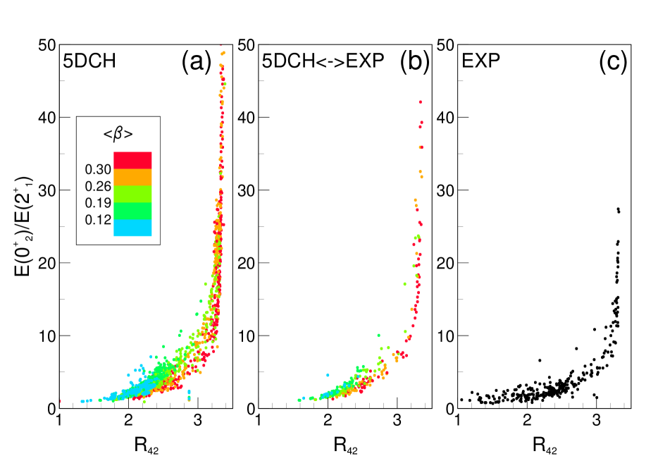
Figure 21: (Color online) Panel (a): ratio $E(0^{+}_{2})/E(2^{+}_{1})$ as a function of $R_{42}$ for the calculated nuclei. Panel (c): experimental data from Ref. brookhaven . Panel (b): CHFB+5DCH values for the nuclei shown in the right-hand panel. Color code is for mean ground state deformation.

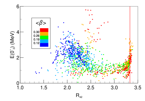
Figure 22: (Color online) CHFB+5DCH excitation energy (MeV) of the $0^{+}_{2}$ state as a function of the ratio $R_{42}$. Color code is for mean ground state deformation. The vertical line (red color) indicates the rotational limit $R_{42}$ = $10/3$.

VI.2.1 Criteria for the occurrence of $\beta$-vibration

As said above, the $0^{+}_{2}$ excitation in nuclei can arise as a $\beta$-vibration, as a coexisting level with deformation different from that for lower-lying states, or something intermediate between these two extreme structures. Here we would like to place the above discussion in a broader perspective.

First we consider relationships between quadrupole transition matrix elements calculated in our theory for the $2^{+}_{1}\rightarrow 0^{+}_{2}$, $2^{+}_{3}\rightarrow 2^{+}_{1}$, and $2^{+}_{3}\rightarrow 0^{+}_{1}$ transitions. If the spectrum truly exhibits a $\beta$-vibrational band, the quadrupole transitions between it and the ground state should be governed by a single parameter, the matrix element of the quadrupole operator between the two intrinsic states. Under these circumstances the spectroscopic transition matrix elements are related by Clebsch-Gordan coefficients, cf. (BM, , Eq. 4-219):

$$\langle\beta J_{\beta}||{\cal M}(E2)||gJ_{g}\rangle=(2J_{g}+1)^{1/2}(J_{g}020|J_{\beta}0)\langle\beta|{\cal M}(E2)|g\rangle.$$ (27)

Here the ground-state and the $\beta$-vibration bands are labeled by $g$ and $\beta$, respectively. We examine now the three CHFB+5DCH cross-band transitions, $(J_{\beta},J_{g})=(0,2),(2,0),(2,2)$, to see how well Eq. (27) is satisfied. According to the model, the magnitudes $|M_{J_{\beta},J_{g}}|$ should satisfy

$$|M_{02}|=|M_{20}|=\sqrt{7\over 10}|M_{22}|.$$ (28)

To display the deviations of the computed matrix elements from these conditions, we take the ratio of the three quantities $|M_{02}|,|M_{20}|,\sqrt{7\over 10}|M_{22}|$ to their total. The fractions are plotted in Fig. 23 as points within a triangle, the fraction given by the distance to a side of the triangle. We see that there is a concentration of points at the center point of the triangle; of the 1707 calculated nuclei, 398 have values of the relative matrix elements within 15% of equality. The distribution of these nuclei in $Z$ and $N$ is shown in Fig.24. One sees four regions where the condition is well satisfied, including the strongly deformed rare earths and actinides.

Figure 23: Crossover matrix elements. Relative magnitudes of the three quantities $|M_{02}|,|M_{20}|,\sqrt{7\over 10}|M_{22}|$ are shown by distances to the sides of the triangle. The vertexes of the triangle correspond to the case where only the labeled transition is nonzero.

We conclude that the CHFB+5DCH theory predicts that $\beta$-vibrational bands should be quite common, taking as a criterion that eq.(26) be approximately satisfied. There is also a concentration of points at the upper apex of the triangle in Fig 23. For these nuclei, the $0^{+}_{2}\rightarrow 2^{+}_{1}$ matrix element is much larger than the two matrix elements involving the $2^{+}_{3}$ excitation, suggesting that the excitations behave more like independent phonons.

Figure 24: Chart of nuclei (full circles) in the vicinity of the center point of the triangle shown in Fig. 23. The continuous curve is for the $\beta$-stability line, and dots are for nuclei between driplines as shown in the left-hand panel of Fig. 3.

VI.2.2 $0^{+}_{2}\rightarrow 2^{+}_{1}$ transition

We now focus on the experimental situation with respect to the $0^{+}_{2}\rightarrow 2^{+}_{1}$ transition strength. This is an important observable in an ongoing controversy about the existence of $\beta$-bands in deformed nuclei Ga01 ; Wi08 .

In Ga01 , it is concluded that the observed $\beta$- to ground state -band transitions are orders of magnitude weaker than those predicted by collective models for deformed rare-earth nuclei, except for very few. To assess the performance of the CHFB+5DCH at least in this limited region, we have compared the CHFB+5DCH calculations of the $B(E2;0^{+}_{2}\rightarrow 2^{+}_{1})$ strengths with the experimental data on the 9 nuclei compiled in Ref. Ga01 . For all of these nuclei, the CHFB+5DCH theory predicts a $\beta$-vibrational band that satisfies the criteria discussed in the previous subsection. For 4 of the nuclei (^152,154Sm, ¹⁵⁴Gd, and ¹⁶⁸Yb), the calculated B(E2)’s are of the same order as the experimental ones, but somewhat higher by up to a factor of 2 or so. However, for the remaining 5 nuclei (¹⁵⁸Gd, ^166,168Er, and ^172,174Yb), the experimental values are an order of magnitude smaller and in strong disagreement with the CHFB+5DCH theory. Thus, for these nuclei at least, the observed band built on the $0^{+}_{2}$ states does not correspond to $\beta$-vibration calculated in the CHFB+5DCH theory.

Recent measurements have shown that many $0^{+}$ excited states are present at low excitation energy in the deformed rare earths me06 . This suggests that the $0^{+}$ levels described by the CHFB+5DCH may be quite fragmented. For example, the $\beta$-vibrational mode couples to such modes as pairing vibrations and/or incoherent 2qp excitations. In the algebraic models, efforts have been made to explain the extra $0^{+}$ states by introducing many-particle many-hole excitations or99 ; he08 . Other regions of deformed nuclei like the actinides and transactinides would be worth investigating to check whether they also are missing the coherent $\beta$-vibrational structure predicted by the CHFB+5DCH theory.

VI.2.3 $0^{+}_{2}\rightarrow 0^{+}_{1}$ transition

Another observable relevant to the structure of the $0^{+}_{2}$ level is its monopole transition strength to the ground state. The strength is conventionally expressed in terms of the quantity $\rho^{2}$ defined as Wo99

$$\rho^{2}(E0;0^{+}_{2}\rightarrow 0^{+}_{1})=|\frac{\langle 0^{+}_{2}|\sum_{i=1}^{Z}r_{i}^{2}|0^{+}_{1}\rangle}{R_{0}^{2}}|^{2},$$ (29)

with $R_{0}=1.2A^{1/3}$ fm. We calculate the required matrix element as

$$\langle 0^{+}_{2}|\sum_{i=1}^{Z}r_{i}^{2}|0^{+}_{1}\rangle=\int da_{0}da_{2}g^{0_{1}}_{0}(a_{0},a_{2})g^{0_{2}}_{0}(a_{0},a_{2})\langle\Phi(a_{0},a_{2})|\sum_{i=1}^{Z}r_{i}^{2}|\Phi(a_{0},a_{2})\rangle.$$ (30)

We find rather interesting systematics with respect to the neutron number as shown in Fig. 25.

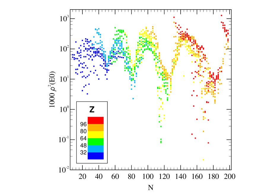
Figure 25: (Color online) Systematics of the calculated squared monopole transition matrix element $\rho^{2}(E_{0};0^{+}_{2}\rightarrow 0^{+}_{1})$ as a function of neutron number $N$. Color code is for proton number.

The calculations display oscillatory structures with broad maxima located near mid-shell closures (N $\simeq$ 40, 64, 100, and 150) and sharp minima in the vicinity of shell closures with N $\simeq$ 20, 28, 50, 82, 126, and 184. Except for light nuclei, all these minima take place for mean ground state deformations $<\beta>$ with small values, that is for spherical equilibrium shapes. These features are globally consistent with IBA calculations for E0 transitions: the $\rho^{2}(E0;0^{+}_{2}\rightarrow 0^{+}_{1})$ values raise sharply in the shape transition regions and then remain large for well deformed nuclei Br04 . Other minima in E0 strengths are found below N $\simeq$ 126 and N $\simeq$ 184 neutron shell closures. Those associated with $N\simeq 162$ and weak $<\beta>$ values are correlated with the opening of the neutron shell closure in transactinide nuclei, as discussed previously in Sec. IV.3. The other two minima take place in open shell nuclei at mean ground state deformation in the ranges $<\beta>\ \simeq$ 0.19-0.26 and $<\beta>\ \simeq$ 0.26-0.30 for neutron numbers $N\simeq 116$ and $N\simeq 158$, respectively. These features as well as similar ones identified in light nuclei with N $\simeq$ 20 and N $\simeq$ 28 indicate that the existence of minima in the E0 strengths over the (N,Z) plane are not exclusively correlated with shell closure and spherical ground states. Finally we note that the E0 strength values are at a maximum near N = 132 and N = 190 and decrease with N increasing. These features are relevant to the Z $>$ 96 isotopic chains for which mean ground state deformations display strong variations (see right-hand panel in Fig. 3).

We have compared our $\rho^{2}(E0)$ transition strengths to 87 of the 91 nuclei tabulated in Ref. ki05 . The result for $R$ figure of merit is given in Table 4. We see that experimental matrix elements are on the average very small compared to theory. This suggests that the experimental $0^{+}_{2}$ levels may have a very different structure than the calculated ones. It may be that configurations ignored by the CHFB+5DCH, such as 2 qp excitations, may be important in the non-yrast spectrum Ta83 . This problem with the parameter-free CHFB+5DCH theory which globally overestimates the E0 strengths by an order of magnitude is shared by other models of nuclear structure. For example, enforcing realistic model descriptions of M1 and E2 transitions or charge radii, it is not uncommon that calculated E0 strengths are up to ten times stronger than experimental values Ze08 ; Bo09 ; Ra09 . The actual nature of E0 transitions remains an elusive issue pointing to major improvements required in structure models.

VI.2.4 Coexistence between bands

We have seen above that the conditions for the occurrence of $\beta$-vibration impose the medium- and heavy-mass deformed nuclei to lay in specific (Z,N) regions (see Fig. 24). One is then left with the issue as to what can be learned on collective excited K = 0 band properties for nuclei which do not belong to this sample. For this purpose we define an important indicator of band structure through the ratio

$$R_{20}(BB^{\prime})=\frac{B(E2;2^{+}_{3}\rightarrow 0^{+}_{2})}{B(E2;2^{+}_{1}\rightarrow 0^{+}_{1})}$$ (31)

for all nuclei of present interest with the provision that $2^{+}_{3}$ levels have preponderant K = 0 component (i.e. P(K = 0) $>$ 0.75) in their wave functions which unambiguously makes them members of excited K = 0 bands. This ratio displays marked structures only if plotted versus neutron number. It is shown in Fig. 26 where open and solid symbols are for $R_{42}\geq 2.3$ and $R_{42}<2.3$, respectively. $R_{20}(BB^{\prime})$ values in the vicinity of $R_{20}(BB^{\prime})$ =1 are representative of the points concentrated at the center point of the triangle shown previously in Fig. 23, and these take place near mid-neutron-closed shell numbers $N=100,150$. Most $R_{20}(BB^{\prime})$’s take on values away from unity. Those with $R_{20}(BB^{\prime})$ $>$ 1 are suggestive of stronger collectivity present in excited K = 0 band than in ground state band, and the other way around for $R_{20}(BB^{\prime})$ $<$ 1 values.

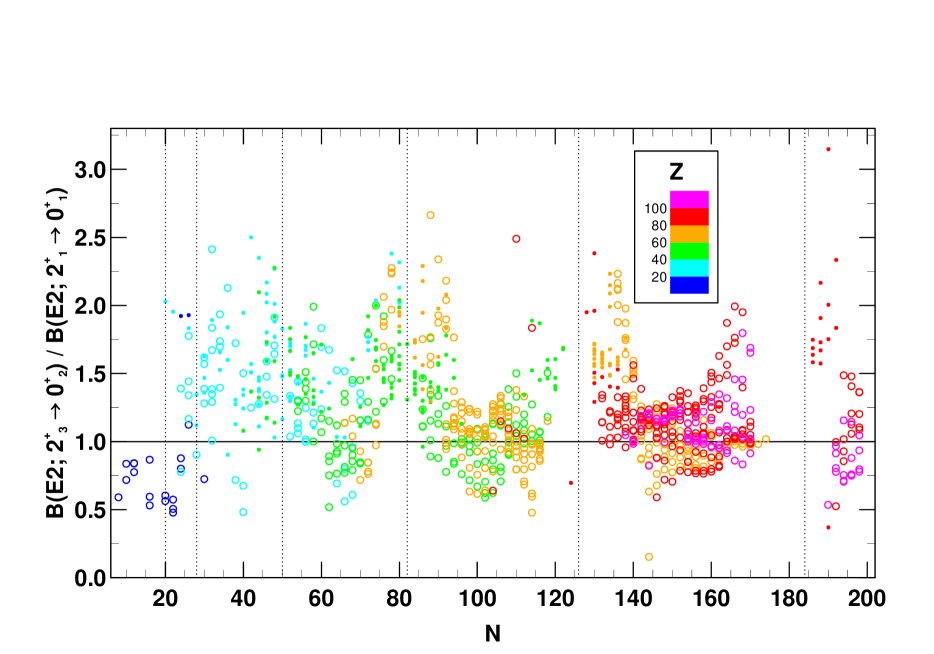
Figure 26: (Color online) The ratio $R_{20}(BB^{\prime})$, Eq. (31), as a function of neutron number. Color code is for proton number. Data marked with open and solid symbols are for $R_{42}\geq 2.3$ and $R_{42}<2.3$, respectively.

It is for N $<$ 60 nuclei that the symbols in Fig. 26 show disparate features as, within a narrow range of N values, $R_{20}(BB^{\prime})$ rapidly flips from $R_{20}(BB^{\prime})$ $>$ 1 to $R_{20}(BB^{\prime})$ $<$ 1. These features have not been analyzed in detail but suggest strong shell effects driving nuclei from near spherical to deformed or from prolate to oblate, or vice versa. A typical example is that offered by the neutron-deficient Kr isotopes which display shape coexistence features, and also undergo a shape transition from prolate to oblate cl07 . Nuclides with N $>$ 60 display less scattered features in their ratios $R_{20}(BB^{\prime})$ which now form a seemingly regular oscillatory trajectory versus N. Extrema are not well localized but undoubtedly they are reasonably close to $N=$ 66, 78, 90, 100, 116, 136, 146, 170 and 196 for nuclei with $R_{42}\geq 2.3$. Detailed information on the location of nuclei with such properties over the (N,Z) plane is not yet available. At this moment we have checked that the ratio $R_{20}(BB^{\prime})$ can serve as good indicator for the identification of nuclei known to display shape coexistence (i.e. isotopes of the Se, Kr, Sr, Zr, Sm, Hg, Pb, and Po elements) associated with the presence of two (or three) minima in potential energy surfaces. Coexistence between collective bands are calculated for Pd, Cd, and Te isotopes which are known experimentally to display such features, see e.g. lh99 . For these nuclides, coexistence is related to well localized maxima in collective masses present at different loci over the $(\beta$,$\gamma$) plane and not to prominent minima in potential energy surfaces. Other theoretical treatments of this kind of coexistence have mostly been based on the Interacting Boson Model, invoking particle-hole excitations between shells to explain the intruder states  ri87 ; Co96 ; Le97 .

VII Summary and Outlook

In this work we have evaluated the performance of the CHFB+5DCH theory based on the Gogny D1S interaction as a global theory of nuclear structure. Highlights of the successes of the theory are its accurate predictions with respect to charge radii, the classification of nuclei as deformed rotors or not, and the ground state band properties of the axial rotors.

The calculated 2-nucleon separation energies are interesting in that they show shell effects and how they are modified for nuclei far from stability. An example is the nuclei near $N,Z=40$. These are often predicted to be spherical in HFB. This is also the case for the Gogny interaction, but we find that there is a change in structure going to the CHFB+5DCH extension, and the nuclei become deformed rotors, in agreement with experiment. The CHFB+5DCH theory is a suitable framework where the issues of shell erosion and shell collapse can be addressed.

As a spectroscopic theory, the CHFB+5DCH has considerable predictive power for the lowest yrast and yrare states, even for nonrotational spectra. This is illustrated by predicted energies of the $2^{+}_{1},4^{+}_{1}$ and $2^{+}_{2}$ excitations, which we compared with compiled empirical data. The performance with respect to the $0^{+}_{2}$ levels also showed predictive power, but here systematic deficiencies of the theory become apparent. All in all, it is quite remarkable that a theory based on a many-body Hamiltonian with only 14 interaction parameters has such predictive power over the broad range of the nuclei that can be treated in the methodology. An important finding is that deformation alone is not a good predictor of rotational spectra. We defined a quantity, $\beta$-softness, that correlates much better. For convenience, we summarize in Table 4 the figures of merit for the performance of the theory for excitation energies and transition properties. We also provide in a retrievable form the specific predictions for spectral properties of about 1700 even-even nuclei and analyzed some of the systematics of the predicted quantities.

Table 4: Summary of the performance statistics of the CHFB+5DCH for excitation energies and transition properties. See text for definitions of $\bar{R}$ and $\sigma$. The column “Number” gives the number of nuclei in the comparison data set.

Observable	Number	$\bar{R}$	$\sigma$
$E(2^{+}_{1})$	513	0.11	0.35
$B(E2;2^{+}_{1}\rightarrow 0^{+}_{1})$	311	0.20	0.42
$R_{42}$	480	0.03	0.14
$R_{62}$	427	0.08	0.21
$E(2^{+}_{2})$	352	0.19	0.30
$E(0^{+}_{2})$	317	0.31	0.36
$\langle 0^{+}_{2}|r_{p}^{2}|0^{+}_{1}\rangle$	$87$	2.1	1.9

There are a number of avenues that could be pursued to improve the theory, some of which are quite straightforward, at least in principle. The treatment of the inertial masses could be improved by using the Thouless-Valatin prescription which is better justified than the cranking approximation we have used up to now. This would surely improve the energies of the $0^{+}_{2}$ excitations, which is one of the problems of the current theory. This would require calculating the QRPA response function at every grid point. This would of course add to the computational burden, but the ingredients to perform the calculation are available for the most part in the intermediate calculations already performed. The rotational inertias could also be improved by using a finite amplitude rotational field $\omega\hat{J}_{k}$ adjusted to self-consistency for the angular momentum value being calculated ma75 . The ingredients of this self-consistent treatment are already available and have been implemented in some calculations Ob05 . This also would considerably add to the computational burden.

We have taken the correlation energy as an indicator of the validity of the Gaussian Overlap Approximation, and excluded nuclei whose calculated correlation energies are unphysical. A better treatment of the correlation energy would include the ZPE term coming from the curvature of the potential energy surface. This term is small in nuclei with broader collective potential energy surfaces, but in noncollective nuclei the minima can be narrow, and this potential term in the Hamiltonian mapping might have a significant effect.

Another deficiency of the CHFB+5DCH that became evident in the discussion of the $0^{+}_{2}$ level properties is the need for 2 qp components in the wave functions. This can be carried out in the GCM if the Hamiltonian operator in the collective space is calculated with full treatment of the nonlocality di76 . However, there is no clear road to us for how to include these components and keep the Gaussian Overlap Approximation as yet.

While it is remarkable that the Hamiltonian based on the Gogny D1S interaction has so much predictive power after 30 years, one can still ask how the calculated observables depend on the intrinsic properties of the Hamiltonian and whether an improvement can be made at that level. We note that there has already been some work to improve the Gogny interaction for calculating nuclear masses, while keeping unaltered the performance of the CHFB+5DCH and RPA theories achieved previously with D1S hilaire .

Finally, as a separate publication, we will present in more detail the spectroscopic properties to higher angular momenta for the deformed rare-earth nuclei. This will also include discussion on the systematics of interband transitions and odd-even angular momentum staggering of the $\gamma$ bands NewWork .

References

- (1) CEA database, http://www-phynu.cea.fr/HFB-5DCH-table.htm, and EPAPS Document No. [number will be inserted by publisher] for tables of predicted properties of even-even nuclei and for color and black and white charts. For more information on EPAPS, see http://www.aip.org/pubservs/epaps.html.
- (2) J. Dechargé and D. Gogny, Phys. Rev. C 21, 1568 (1980).
- (3) J.-F. Berger, M. Girod, and D. Gogny, Comp. Phys. Comm. 63, 365 (1991).
- (4) G.F. Bertsch, M. Girod, S. Hilaire, J.-P. Delaroche, H. Goutte, and S. Péru, Phys. Rev. Lett. 99, 032502 (2007).
- (5) F. Chappert, M. Girod, and S. Hilaire, Phys. Lett. B668, 420 (2008); S. Goriely, S. Hilaire, M. Girod and S. Péru, Phys. Rev. Lett. 102, 242501 (2009).
- (6) N. Tajima, S. Takahara, N. Onishi, Nucl. Phys. A603 (1996).
- (7) G. A. Lalazissis, M. M. Sharma, P. Ring, Nucl. Phys. A597, 35 (1996).
- (8) P. Klüpfel, J. Erler, P.-G. Reinhard, and J.A. Maruhn, Eur. Phys. J. A 37 343 (2008).
- (9) T. Nikšić, et al., Phys. Rev. 79 034303 (2009).
- (10) A. Valor, P.-H. Heenen, and P. Bonche, Nucl. Phys. A 671 145 (2000).
- (11) R.R. Rodríguez-Guzmán, J.L. Egido and L.M. Robledo, Phys. Rev. C62 054319 (2000); Phys. Rev. C 65 024304 (2002).
- (12) M. Bender, G.F. Bertsch, and P.-H. Heenen, Phys. Rev. C 73, 034322 (2006).
- (13) B. Sabbey, M. Bender, G.F. Bertsch, and P.H. Heenen, Phys. Rev. C 75 044305 (2007).
- (14) J.Terasaki, J. Engel, and G.F. Bertsch, Phys. Rev. C 78, 044311 (2008).
- (15) M. Stanoiu et al., Phys. Rev. C 69, 034312 (2004).
- (16) S. Péru, M. Girod, and J.-F. Berger, Eur. Phys. J. A9, 35 (2000).
- (17) A. Obertelli, S. Péru, J.-P. Delaroche, A. Gillibert, M. Girod, and H. Goutte, Phys. Rev. C 71, 024304 (2005).
- (18) J. Libert, M. Girod, and J.-P. Delaroche, Phys. Rev. C 60, 054301 (1999) and references therein.
- (19) M. Girod and B. Grammaticos, Phys. Rev. C 27, 2317 (1983).
- (20) J.-F. Berger, Ph.D. thesis, Université de Paris-Sud, 1985.
- (21) K. Kumar and M. Baranger, Nucl. Phys. A92, 608 (1967).
- (22) M. Girod and B. Grammaticos, Nucl. Phys. A330, 40 (1979).
- (23) E. Clément et al., Phys. Rev. C 75, 054313 (2007).
- (24) Brookhaven database, http://www.nndc.bnl.gov/
- (25) M.Girod, J.-P.Delaroche, A.Gorgen and A.Obertelli, Phys.Lett. B 676, 39 (2009)
- (26) F. Iachello, N. V. Zamfir, and R. F. Casten, Phys. Rev. Lett. 81, 1191 (1998).
- (27) Z.P. Li, T. Nikšić, D. Vretenar, J. Meng, G.A. Lalazissis, and P. Ring, Phys. Rev. C 79, 054301 (2009) and references therein.
- (28) F. Iachello, Phys. Rev. Lett. 87, 052502 (2001).
- (29) R.F. Casten and N.V. Zamfir, Phys. Rev. Lett. 87, 052503 (2001).
- (30) R.F. Casten and E. A. McCutchan, J. Phys. G : Nucl. Part. Phys. 34, R285 (2007).
- (31) W.D. Kulp et al., Phys. Rev. C 76, 034319 (2007).
- (32) N.V. Zamfir et al, Phys. Rev. C 60, 054312 (1999).
- (33) T. Klug, A. Dewald, V. Werner, P. von Brentano, and R.F. Casten, Phys. Lett. B495, 55 (2000).
- (34) R. Bijker, R.F. Casten, N.V. Zamfir, and E.A. McCutchan, Phys. Rev. C 68, 064304 (2003).
- (35) W.D. Kulp et al, Phys. Rev. C 71, 041303(R) (2005).
- (36) R. F. Casten, private communication.
- (37) http://massexplorer.com; in their SLy4 data set the fraction of oblate nuclei among the deformed nuclei is 23%.
- (38) I. Angeli, Atomic Data Nuclear Data Tables 87, 185 (2004).
- (39) For the Sr and Zr isotopic chains, we used the data of Refs. ca02 ; bu00 to determine the experimental radii, taking the values of 88Sr and 90Zr from Ref. an04 .
- (40) J. Negele, Phys. Rev. C 1, 1260 (1970).
- (41) I. Angeli, private communication.
- (42) E.W. Otten, Treatise on Heavy Ion Science, D.A. Bromley, ed. (Plenum, NY 1980), Vol. 8.
- (43) N. Tajima, P. Bonche, H. Flocard, P.-H. Heenen, and M.S. Weiss, Nucl. Phys. A551, 434 (1993).
- (44) P.-G. Reinhard and H. Flocard, Nucl. Phys. A584, 467 (1995).
- (45) M.M. Sharma, G. Lalazissis, J. König, and P. Ring, Phys. Rev. Lett. 74, 3744 (1995).
- (46) F. Buchinger et al., Phys. Rev. C 41, 2883 (1990).
- (47) P. Campbell et al., Phys. Rev. Lett. 89, 082501 (2002).
-
(48)
http://pdg.lbl.gov/2008/listings/so16.pdf
http://pdg.lbl.gov/2008/listings/so17.pdf - (49) G. Audi, A.H. Wapstra, and C. Thibault, Nucl. Phys. A729, 337 (2003).
- (50) M. Bender, G.F. Bertsch, and P.-H. Heenen, Phys. Rev. C 78, 054312 (2008).
- (51) R. Smolanczuk, J. Skalski, and A. Sobiczewski, Phys. Rev. C 52,1871 (1995).
- (52) Y. Oganessian, J. Phys. G: Nucl. Part. Phys. 34, R165 (2007).
- (53) D. S. Brenner, N. V. Zamfir, and R. F. Casten, Phys. Rev. C 50, 490 (1994); ibid. 55, 974 (1997); P.D.Cottle and N. V. Zamfir, Phys. Rev. C 58, 1500 (1998).
- (54) D. Lunney, J. M. Pearson, and C. Thibault, Rev. Mod. Phys. 75, 1021 (2003).
- (55) A.M. Lane, Nuclear Theory-Pairing Correlations and Collective Motion (Benjamin, Reading, MA, 1964), p. 80.
- (56) S. Raman, C.W. Nestor, and P. Tikkanen, At. Data Nucl. Data Tables 78, 1 (2001).
- (57) J.A. Shannon et al., Phys. Lett. B336, 136 (1994).
- (58) J. Libert and P. Quentin, Z. Phys. A306, 315 (1982).
- (59) R.F. Casten, Nuclear Structure from a Simple Perspective, 2nd ed. (Oxford University Press, Oxford, 2000).
- (60) C.A. Mallmann, Phys. Rev. Lett. 2 507 (1959).
- (61) D. Bucurescu, N.V. Zamfir, G. Cata-Danil, M. Ivascu, N.Marginean, Phys. Rev. C78 044322 (2008).
- (62) M. Bender and P.-H. Heenen, Nucl. Phys. A713, 390 (2003).
- (63) M. Bender, H. Flocard, and P.-H. Heenen, Phys. Rev. C 68, 044321 (2003).
- (64) J.-P. Delaroche, M. Girod, H. Goutte, and J. Libert, Nucl.Phys. A771, 103 (2006).
- (65) S.J. Krieger, P. Bonche, M.S. Weiss, J. Meyer, H. Flocard, and P.-H. Heenen, Nucl. Phys. A542, 43 (1992).
- (66) S. Takahara, N. Tajima, and N. Onishi, Nucl. Phys. A642 461, (1998).
- (67) M. Girod, J.-P. Delaroche, A. Gorgen, and A. Obertelli, Phys. Lett. B 676, 39 (2009).
- (68) W.-T. Chou, Gh. Cata-Danil, N.V. Zamfir, R.F. Casten, and N. Pietralla, Phys. Rev. C 64, 057301 (2001).
- (69) A. Bohr and B. Mottelson, Nuclear Structure (Benjamin, Reading, MA, 1975), Vol.II.
- (70) P.E. Garrett, J. Phys. G: Nucl. Part. Phys. 27, R1 ((2001).
- (71) K. Wimmer et al., arXiV:0802.2514.
- (72) D. A. Meyer et al., Phys. Rev. C 74, 044309 (2006); Phys. Lett. B638, 44 (2006).
- (73) A. M. Oros, K. Heyde, C. De Coster, B. Decroix, R. Wyss, B.R. Barrett, and P. Navratil, Nucl. Phys. A645, 107 (1999).
- (74) V. Hellemans, S. De Baerdemacker, and K. Heyde, Phys. Rev. C 77, 064324 (2008).
- (75) J. L. Wood, E.F. Zganjar, C. De Coster, and K. Heyde, Nucl. Phys. A651, 323 (1999).
- (76) P. von Brentano, V. Werner, R.F. Casten, C. Scholl, E.A. McCutchan, R. Krucken, and J. Jolie, Phys. Rev. Lett. 93, 152502 (2004).
- (77) T. Kibedi and R.H. Spear, At. Data Nucl. Data Tables 89, 77 (2005).
- (78) K. Takada and S. Tazaki, Nucl. Phys. A395, 165 (1983) and references therein.
- (79) S. Zerguine, P. Van Isacker, A. Bouldjedri, and S. Heinze, Phys. Rev. Lett. 101, 022502 (2008).
- (80) J. Bonnet, A. Krugmann, J. Beller, N. Pietralla, and R. V. Jolos, Phys. Rev. C 79, 034307 (2009).
- (81) A.A. Raduta, C.M. Raduta, E; Moya de Guerra, and P. Sarriguren, J. Phys. G: Nucl. Part. Phys. 36, 015114 (2009).
- (82) G. Lhersonneau, J.C. Wang, S. Hankonen, P. Dendooven, P. Jones, R. Julin, and J. Aysto, Phys. Rev. C 60, 014315 (1999).
- (83) J. Rikovska, N. J. Stone, and W. B. Walters, Phys. Rev. C 36, 2162 (1987).
- (84) C. De Coster, K. Heyde, B. Decroix, P. Van Isacker, J. Jolie, H. Lehmann, and J.L. Wood, Nucl. Phys. A600, 251 (1996); ibid. 621, 802 (1997); ibid. 651, 31 (1999).
- (85) H. Lehmann, J. Jolie, C. De Coster, B. Decroix, K. Heyde, and J.L. Wood, Nucl. Phys. A621, 767 (1997).
- (86) H. Mang, Phys. Reports 18, 325 (1975).
- (87) M. Didong, H. Müther, K. Goeke, and A. Faessler, Phys. Rev. C 14, 1189 (1976).
- (88) J.-P. Delaroche et al., in preparation.