Krylov subspace methods and the sign function: multishifts and deflation in the non-Hermitian case

Abstract:

Rational approximations of the matrix sign function lead to multishift methods. For non-Hermitian matrices long recurrences can cause storage problems, which can be circumvented with restarts. Together with deflation we obtain efficient iterative methods, as we show in numerical experiments for the overlap Dirac operator at non-vanishing quark chemical potential for lattices up to size $10^{4}$.

1 Introduction

In this paper we discuss the approximation of $f(A)b$, where $A\in{\mathbb{C}}^{n\times n}$ is non-Hermitian and $f$ is a function defined on the spectrum of $A$ such that the extension of $f$ to matrix arguments is defined.

The motivation for this rather general setting comes from quantum chromodynamics (QCD) formulated on a discrete space-time lattice, where $f=\operatorname{sign}$ is of special interest. As the main object relevant for our discussion we are focusing on the overlap Dirac operator [3, 4]. The main numerical effort lies in the inversion of the overlap operator, which is done by iterative methods and requires the repeated application of the sign function of the usual “symmetrized” Wilson operator $H_{W}=\gamma_{5}D_{W}$ (see [5] for the notation) on a vector.

At zero quark chemical potential $\mu$, the operator $H_{W}$ is Hermitian. However, one can also study QCD at nonzero $\mu$, which is relevant for many physical systems such as neutron stars, relativistic heavy ion collisions, or the physics of the early universe. The overlap operator has been generalized to this case [5, 6]. The computational challenge is the fact that at non-zero chemical potential $H_{W}$ becomes non-Hermitian.

This contribution is organized as follows. In Section 2 we review multishift methods which have proven to be successful in the Hermitian ($\mu=0$) case. We will point out the problems that occur when applying these methods to the non-Hermitian ($\mu\neq 0$) case. In Sections 3 and 4 we present two procedures, restarts and deflation, which — especially when applied in combination — make multishift methods applicable to non-Hermitian matrices. We present our numerical results in Section 5, and conclusions are drawn in Section 6.

2 Multishift methods

First we recall some results for the Hermitian case, i.e., we investigate the computation of $f(A)b$, where $A\in{\mathbb{C}}^{n\times n}$ is Hermitian. If $A$ is large, $f(A)$ is too costly to compute, while $f(A)b$ can still be obtained in an efficient manner if $A$ is sparse. Krylov subspace methods, i.e., methods that approximate $f(A)b$ in a Krylov subspace $K_{k}(A,b)=$span$\{b,Ab,\dots,A^{k-1}b\}$, are suitable for this task. We distinguish between two Krylov subspace approaches: direct projection and multishift.

Direct projection methods compute the sign function for the projection of $A$ onto $K_{k}(A,b)$ and lift the result back to the original space, see [1, 7], or [8, 9] in the context of QCD. These methods are not the topic of this paper, but we will use them for comparison in our numerical results.

The idea of multishift methods is to approximate $f$ by a rational function $g$,

$$f(x)\approx g(x)=\sum\limits_{i=1}^{s}\frac{\omega_{i}}{x-\sigma_{i}}\,.$$ (1)

The systems

$$(A-\sigma_{i}I)x^{(i)}=b\,,\quad i=1,\dots,s$$ (2)

are treated with standard Krylov subspace methods such as the conjugate gradient method (CG) or the minimal residual method (MINRES), approximating $x^{(i)}$ by ${x_{k}}^{(i)}$ from a Krylov subspace. Since Krylov subspaces are shift invariant, i.e., $K_{k}(A-\sigma_{i}I,b)=K_{k}(A,b)$, the approximations ${x_{k}}^{(i)}$ can be computed simultaneously using the same subspace for all systems. The desired approximation is then obtained by combining the approximations to the $s$ shifted systems

$$f(A)b\approx x_{k}=\sum\limits_{i=1}^{s}\omega_{i}{x_{k}}^{(i)}\,.$$ (3)

The core of any such method is the computation of an appropriate basis for the Krylov subspace. For Hermitian matrices an orthonormal basis can be built with short recurrences using the Lanczos process. These short recurrences are essential for the efficiency of the approach.

Turning to non-Hermitian matrices, the computation of an orthogonal basis now requires long recurrences and is usually summarized via the Arnoldi relation

$$AV_{k}=V_{k}H_{k}+h_{k+1,k}v_{k+1}e_{k}^{T}\,.$$ (4)

Here, $V_{k}=\left[v_{1}|\dots|v_{k}\right]\in{\mathbb{C}}^{n\times k}$ is the matrix which contains the computed basis vectors (the Arnoldi vectors), $H_{k}={V_{k}}^{\dagger}AV_{k}$ is the upper Hessenberg matrix containing the recurrence coefficients $h_{i,j}$, and $e_{k}$ denotes the $k$-th unit vector of ${\mathbb{C}}^{k}$.

For the rational approximation approach this means that the short-recurrence methods CG and MINRES have to be replaced by multishift versions of the corresponding long-recurrence methods, i.e., the full orthogonalization method (FOM) [10] and the generalized minimal residual method (GMRES) [11], respectively.

Long recurrences slow down computation and increase storage requirements, and thus become inefficient or even infeasible if $k$, the dimension of the Krylov subspace, becomes large. In this paper we investigate restarts to circumvent this problem for non-Hermitian matrices.

3 Restarts

FOM to solve $Ax=b$ consists of the Arnoldi process to compute the Arnoldi vectors $v_{1},\dots,v_{k}$ as well as the upper Hessenberg matrix $H_{k}={V_{k}}^{\dagger}AV_{k}$ and of approximating $x\approx x_{k}=\|b\|_{2}V_{k}{H_{k}}^{-1}e_{1}$. The Arnoldi process applied to $A-\sigma_{i}I$ instead of $A$ produces the same matrices $V_{k}$ with $H_{k}$ replaced by the shifted counterpart $H_{k}-\sigma_{i}I$. The $k$-th approximation to $g(A)b$, with $g(x)$ defined in (1), is thus given by $\|b\|_{2}\sum_{i=1}^{s}V_{k}(H_{k}-\sigma_{i}I)^{-1}e_{1}$.

To prevent recurrences from becoming too long one can — in this case — use a restart procedure. This means that one stops the Arnoldi process after $k_{\text{max}}$ iterations. At this point we have a, possibly crude, approximation to $g(A)b$, and to allow for a restart one now has to express the error of this approximation anew as the action of a matrix function, $g_{1}(A)b_{1}$, say.

A crucial observation concerning multishifts is that for any $k$ the individual residuals ${r_{k}}^{(i)}=b-(A-\sigma_{i}I){x_{k}}^{(i)}$ of the FOM iterates ${x_{k}}^{(i)}$ are just scalar multiples of the Arnoldi vector $v_{k+1}$, see, e.g., [10, 12], i.e.,

$${r_{k}}^{(i)}={\rho_{k}}^{(i)}v_{k+1}\,,\quad i=1,\dots,s$$ (5)

with collinearity factors ${\rho_{k}}^{(i)}\in{\mathbb{C}}$. The error $\Delta_{k}=g(A)b-x_{k}$ of the multishift approximation at step $k$ can therefore be expressed as

$$\Delta_{k}=g_{1}(A)b_{1}\,,\quad\text{where }g_{1}(t)=\sum_{i=1}^{s}\frac{\omega_{i}{\rho_{k}}^{(i)}}{t-\sigma_{i}}\text{ and }b_{1}=v_{k+1}\,.$$ (6)

This allows for a simple restart at step $k_{\text{max}}$ of the Arnoldi process, with the new function $g_{1}$ again being rational with the same poles as $g$. This restart process can also be regarded as performing restarted FOM for each of the individual systems $(A-\sigma_{i}I)x=b$, $i=1,\ldots,s$ (and combining the individual iterates appropriately), the point being that, even after a restart, we need only a single Krylov subspace for all $s$ systems, see [10].

There also exists a restarted version of multishift GMRES, see [11] for a detailed derivation.

4 Deflation

In [8] two deflation approaches were proposed which use eigensystem information, namely Schur vectors (Schur deflation) or left and right eigenvectors (LR deflation) corresponding to some “critical” eigenvalues. Critical eigenvalues are those which are close to a singularity of $f$. If they are not reflected very precisely in the Krylov subspace, we get a poor approximation. In case of the sign function the critical eigenvalues are those close to the imaginary axis. Here, we describe LR deflation (see [13] for the reason why this is the method of choice) and show how it can be combined with multishifts and restarts.

Let $R_{m}=\left[r_{1}|\dots|r_{m}\right]$ be the matrix containing the right eigenvectors and ${L_{m}}^{\dagger}=\left[l_{1}|\dots|l_{m}\right]^{\dagger}$ the matrix containing the left eigenvectors corresponding to $m$ critical eigenvalues of the matrix $A$. This means that we have

$$AR_{m}=R_{m}\Lambda_{m}\quad\text{and}\quad{L_{m}}^{\dagger}A=\Lambda_{m}{L_{m}}^{\dagger}\,,$$ (7)

where $\Lambda_{m}$ is a diagonal matrix containing the $m$ critical eigenvalues. Since left and right eigenvectors are biorthogonal, we can normalize them such that ${L_{m}}^{\dagger}R_{m}=I_{m}$. The matrix $P=R_{m}{L_{m}}^{\dagger}$ represents an oblique projector onto the subspace $\Omega_{R}=\operatorname{span}\{r_{1},\dots,r_{m}\}$.

We now split $f(A)b$ into the two parts

$$f(A)b=f(A)(Pb)+f(A)(I-P)b\,.$$ (8)

Since we know the left and right eigenvectors which make up $P$, we directly obtain

$$x_{P}\equiv f(A)(Pb)=f(A)R_{m}L_{m}^{\dagger}b=R_{m}f(\Lambda_{m})(L_{m}^{\dagger}b)\,,$$ (9)

which can be computed exactly. The remaining part $f(A)(I-P)b$ can then be approximated iteratively by using a multishift method. Thus $f(A)b$ is now approximated in augmented Krylov subspaces $\Omega_{R}+K_{k}(A,(I-P)b)$,

$$x_{k}=\underbrace{x_{P}\phantom{\Bigg{|}}\!\!\!\!}_{\in\Omega_{R}}+\;\;\underbrace{\sum_{i=1}^{s}\omega_{i}x_{k}^{(i)}}_{\makebox[0.0pt]{\scriptsize$\in K_{k}(A,(I-P)b)$}}\,.$$ (10)

Theoretically, we have

$$K_{k}(A,(I-P)b)=(I-P)K_{k}(A,(I-P)b)\subseteq\operatorname{range}(I-P)\,,$$ (11)

see [13]. In computational practice, however, components outside of $\operatorname{range}(I-P)$ will show up gradually when building $K_{k}(A,(I-P)b)$ due to rounding effects in floating-point arithmetic. It is thus necessary to reapply $I-P$ from time to time in order to eliminate these components.

Since the only effect of LR deflation is the replacement of $b$ by $(I-P)b$, no modifications of the restart algorithm are necessary.

5 Algorithms

We combine multishift methods with restarts and deflation. We assume that the original function $f$ is replaced by a rational function (given by the shifts $\sigma_{i}$ and weights $\omega_{i}$) which approximates the original function sufficiently well after deflation.

Depending on the underlying multishift method (FOM or GMRES), we get LR-deflated multishift FOM (FOM-LR) or LR-deflated multishift GMRES (GMRES-LR). Algorithm 1 gives an algorithmic description of FOM-LR. (For an algorithmic description of GMRES-LR we refer to [13].) The notation FOM-LR($m,k$) indicates that we LR-deflate a subspace of dimension $m$ and that we restart FOM after a cycle of $k$ iterations. The vector $x$ is the approximation to $f(A)b$. After the completion of each cycle we perform a projection step to eliminate numerical contamination by components outside of $\operatorname{range}(I-P)$.

Algorithm 1

Restarted FOM-LR($m,k$)

  {Input $m$, $k=k_{\text{max}}$, $A$, $\{\sigma_{1},\dots,\sigma_{s}\}$, $\{\omega_{1},\ldots,\omega_{s}\}$, $b$, $L=L_{m}$, $R=R_{m}$, $\Lambda=\Lambda_{m}$}

  $x=x_{P}=Rf(\Lambda){L}^{\dagger}b$

  $r=(I-P)b$

  $\rho^{(i)}=1$, $i=1,\dots,s$

  while not all systems are converged do {loop over restart cycles}

     $\beta=\|r\|_{2}$

     $v_{1}=r/\beta$

     compute $V_{k}$, $H_{k}$ by running $k$ steps of Arnoldi with $A$

     $y_{k}^{(i)}=\beta\rho^{(i)}(H_{k}-\sigma_{i}I_{k})^{-1}e_{1}$, $i=1,\dots,s$

     $x=x+V_{k}\sum_{i=1}^{s}\omega_{i}y_{k}^{(i)}$

     $r=v_{k+1}$

     $\rho^{(i)}=-h_{k+1,k}e_{k}^{T}y_{k}^{(i)}$, $i=1,\dots,s$

     $r=(I-P)r$ {projection step}

  end while

Note that a combination of deflation and a multishift method based on the two-sided Lanczos algorithm is also possible, see [13]. Of course, since two-sided Lanczos already gives short recurrences, there is no need to restart here.

6 Numerical results

For our numerical experiments we turn to $f=\operatorname{sign}$. In the Hermitian case, the sign function of $A$ can be approximated using the Zolotarev best rational approximation, see [14] and, e.g., [15, 16]. Using the Zolotarev approximation on non-Hermitian matrices gives rather poor results, unless all eigenvalues are close to the real axis. A better choice for generic non-Hermitian matrices is the rational approximation originally suggested by Kenney and Laub [17] and used by Neuberger [18, 19] for vanishing chemical potential,

$$\operatorname{sign}(t)\approx g_{s}(t)\,,\quad\text{where }g_{s}(t)=\frac{(t+1)^{2s}-(t-1)^{2s}}{(t+1)^{2s}+(t-1)^{2s}}\,.$$ (12)

The partial fraction expansion of $g_{s}$ is known to be

$$g_{s}(t)=t\sum_{i=1}^{s}\frac{\omega_{i}}{t^{2}-\sigma_{i}}\quad\text{with }\omega_{i}=\frac{1}{s}\cos^{-2}\left(\frac{\pi}{2s}\left(i-\frac{1}{2}\right)\right),\quad\sigma_{i}=-\tan^{2}\left(\frac{\pi}{2s}\left(i-\frac{1}{2}\right)\right),$$ (13)

see [17, 18]. Note that actually one uses $g(ct)$, where the parameter $c>0$ is chosen to minimize the number of poles $s$ needed to achieve a given accuracy. If the spectrum of $A$ is known to be contained in the union of two circles $C(m,r)\cup C(-m,r)$, where $C(m,r)$ is the circle $\{|z-m|\leq r\}$ and $m$ and $r$ are real with $0<r<m$, then $c=((m+r)(m-r))^{-1/2}$ is optimal, see [13, 16].

Figure 1 shows the performance of FOM-LR in comparison to the direct projection method. The $k$-th approximation in the latter is given as

$$x_{P}+\|(I-P)b\|_{2}V_{k}\operatorname{sign}(H_{k})e_{1}\,,$$ (14)

where $\operatorname{sign}(H_{k})$ is computed via Roberts’ method, see [1]. The relative performance of the two approaches depends on the parameters of the problem, such as the lattice size, the deflation gap, and the size of the Krylov subspace. For more details, see [13]. We add that in the meantime an improved method to compute $\operatorname{sign}(H_{k})$ in the direct approach has been developed, see [20] in these proceedings.

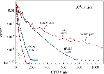
Figure 1: Comparison of the accuracy of the restarted FOM-LR algorithm (rFOM) and the direct two-sided Lanczos-LR method (2sL) as a function of the CPU time in seconds for an $8^{4}$ (left) and a $10^{4}$ (right) lattice configuration, using $\mu=0.3$ in both cases. Each plot shows data for two different deflation gaps, given in parentheses. The restart size used in the restarted FOM-LR algorithm is $k_{\text{max}}=30$ for the $8^{4}$ lattice and $k_{\text{max}}=40$ for the $10^{4}$ lattice.

Figure 2 is meant to convey a warning. It shows that the projection step after each restart, as formulated in Algorithm 1, may be crucial to ensure convergence. In both plots we give results for Algorithm 1 and a variant thereof in which the projection step is omitted. The right plot shows that this may destroy convergence, the left plot shows that this is not necessarily so. Since the CPU time is increased only marginally by the projection step, the latter should always be included.

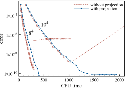
Figure 2: Error vs CPU time for the FOM-LR algorithm with and without re-orthogonalization for $4^{4}$ and $6^{4}$ (left) as well as $8^{4}$ and $10^{4}$ (right) lattices. We again used $\mu=0.3$ in all cases.

7 Conclusion

We have presented an algorithm, FOM-LR, to approximate the action of the sign function of a non-Hermitian matrix on a vector. This algorithm combines LR deflation and a rational approximation to the sign function, which is computed by a restarted multishift method. The latter has fixed storage requirements determined by the restart parameter (maximum size of the Krylov subspace) and the degree of the rational approximation. Occasionally, additional projections of the Krylov vectors are necessary for numerical stability.

Whether FOM-LR or a direct method (i.e., the two-sided Lanczos-LR method) performs better depends on many details of the problem. Some of them have been mentioned in Section 6. Others include implementation issues such as optimized linear algebra libraries, and ultimately parallelization.

References

- [1] N. J. Higham, Functions of Matrices: Theory and Computation. Society for Industrial and Applied Mathematics, 2008.
- [2] A. Frommer and V. Simoncini, Matrix Functions, vol. 13 of Mathematics in Industry, ch. 3, pp. 275–303. Springer, Heidelberg, 2008.
- [3] R. Narayanan and H. Neuberger, A construction of lattice chiral gauge theories, Nucl. Phys. B443 (1995) 305–385, [hep-th/9411108].
- [4] H. Neuberger, Exactly massless quarks on the lattice, Phys. Lett. B417 (1998) 141–144, [hep-lat/9707022].
- [5] J. C. R. Bloch and T. Wettig, Overlap Dirac operator at nonzero chemical potential and random matrix theory, Phys. Rev. Lett. 97 (2006) 012003, [hep-lat/0604020].
- [6] J. C. R. Bloch and T. Wettig, Domain-wall and overlap fermions at nonzero quark chemical potential, Phys. Rev. D76 (2007) 114511, [arXiv:0709.4630].
- [7] H. van der Vorst, An iterative solution method for solving , using Krylov subspace information obtained for the symmetric positive definite matrix A, J. Comput. Appl. Math. 18 (1987) 249–263.
- [8] J. C. R. Bloch, A. Frommer, B. Lang, and T. Wettig, An iterative method to compute the sign function of a non- Hermitian matrix and its application to the overlap Dirac operator at nonzero chemical potential, Comput. Phys. Commun. 177 (2007) 933–943, [arXiv:0704.3486].
- [9] J. C. R. Bloch, T. Breu, and T. Wettig, Comparing iterative methods to compute the overlap Dirac operator at nonzero chemical potential, PoS LATTICE2008 (2008) 027, [arXiv:0810.4228].
- [10] V. Simoncini, Restarted full orthogonalization method for shifted linear systems, BIT Numerical Mathematics 43 (2003) 459–466.
- [11] A. Frommer and U. Glässner, Restarted GMRES for shifted linear systems, SIAM J. Sci. Comput. 19 (1998) 15–26.
- [12] A. Frommer, BiCGStab(l) for families of shifted linear systems, Computing 70 (2003) 87–109.
- [13] J. C. R. Bloch, T. Breu, A. Frommer, S. Heybrock, K. Schäfer, and T. Wettig, Short-recurrence Krylov subspace methods for the overlap Dirac operator at nonzero chemical potential, arXiv:0910.1048.
- [14] E. I. Zolotarev, Application of elliptic functions to the question of functions deviating least and most from zero, Zap. Imp. Akad. Nauk. St. Petersburg 30 (1877) 5.
- [15] D. Ingerman, V. Druskin, and L. Knizhnerman, Optimal finite difference grids and rational approximations of the square root. I. Elliptic problems, Comm. Pure Appl. Math. 53 (2000) 1039–1066.
- [16] J. van den Eshof, A. Frommer, T. Lippert, K. Schilling, and H. A. van der Vorst, Numerical methods for the QCD overlap operator. I: Sign-function and error bounds, Comput. Phys. Commun. 146 (2002) 203–224, [hep-lat/0202025].
- [17] C. Kenney and A. Laub, A hyperbolic tangent identity and the geometry of Padé sign function iterations, Numer. Algorithms 7 (1994) 111–128.
- [18] H. Neuberger, A practical implementation of the overlap Dirac operator, Phys. Rev. Lett. 81 (1998) 4060–4062, [hep-lat/9806025].
- [19] H. Neuberger, The overlap Dirac operator, in Numerical challenges in Lattice Quantum Chromodynamics (A. Frommer, T. Lippert, B. Medeke, and K. Schilling, eds.), pp. 1–17, Springer Berlin, 2000. hep-lat/9910040.
- [20] J. C. R. Bloch and S. Heybrock, A nested Krylov subspace method for the overlap operator, PoS LAT2009 (2009) 025, [arXiv:0910.2918].