Measuring the convergence of Monte Carlo free energy calculations

Abstract

The nonequilibrium work fluctuation theorem provides the way for calculations of (equilibrium) free energy based on work measurements of nonequilibrium, finite-time processes and their reversed counterparts by applying Bennett’s acceptance ratio method. A nice property of this method is that each free energy estimate readily yields an estimate of the asymptotic mean square error. Assuming convergence, it is easy to specify the uncertainty of the results. However, sample sizes have often to be balanced with respect to experimental or computational limitations and the question arises whether available samples of work values are sufficiently large in order to ensure convergence. Here, we propose a convergence measure for the two-sided free energy estimator and characterize some of its properties, explain how it works, and test its statistical behavior. In total, we derive a convergence criterion for Bennett’s acceptance ratio method.

I Introduction

Many methods have been developed in order to estimate free energy differences, ranging from thermodynamic integration Kirkwood1935 ; Gelman1998 , path sampling Minh2009 , free energy perturbation Zwanzig1954 , umbrella sampling Torrie1977 ; Chen1997 ; Oberhofer2008 , adiabatic switching Watanabe1990 , dynamic methods Sun2003 ; Ytreberg2004 ; Jarzynski2006 ; Ahlers2008 , optimal protocols Then2008 ; Geiger2010 , asymptotic tails vonEgan-Krieger2008 , to targeted and escorted free energy perturbation Meng2002 ; Jarzynski2002 ; Oberhofer2007 ; Vaikuntanathan2008 ; Hahn2009a . Yet, the reliability and efficiency of the approaches have not been considered in full depth. Fundamental questions remain unanswered Lu2007 , e.g., what method is best for evaluating the free energy? Is the free energy estimate reliable and what is the error in it? How can one assess the quality of the free energy result when the true answer is unknown? Generically, free energy estimators are strongly biased for finite sample sizes, such that the bias constitutes the main source of error of the estimates. Moreover, the bias can manifest itself in a seemingly convergence of the calculation by reaching a stable value, although far apart from the desired true value. Therefore, it is of considerable interest to have reliable criteria for the convergence of free energy calculations.

Here we focus on the convergence of Bennett’s acceptance ratio method. Thereby, we will only be concerned with the intrinsic statistical errors of the method and assume uncorrelated and unbiased samples from the work densities. For incorporation of instrument noise, see Ref. Maragakis2008 .

With emerging results from nonequilibrium stochastic thermodynamics, Bennett’s acceptance ratio method Bennett1976 ; Meng1996 ; Kong2003 ; Shirts2008 has revived actual interest.

Recent research has shown that the isothermal free energy difference $\Delta f=f_{1}-f_{0}$ of two thermal equilibrium states $0$ and $1$, both at the same temperature $T$, can be determined by externally driven nonequilibrium processes connecting these two states. In particular, if we start the process with the initial thermal equilibrium state $0$ and perturb it towards $1$ by varying the control parameter according to a predefined protocol, the work $w$ applied to the system will be a fluctuating random variable distributed according to a probability density $p_{0}(w)$. This direction will be denoted with forward. Reversing the process by starting with the initial equilibrium state $1$ and perturbing the system towards $0$ by the time reversed protocol, the work $w$ done $by$ the system in the reverse process will be distributed according to a density $p_{1}(w)$. Under some quite general conditions, the forward and reverse work densities $p_{0}(w)$ and $p_{1}(w)$ are related to each other by Crooks fluctuation theorem Crooks1999 ; Campisi2009

$$\frac{p_{0}(w)}{p_{1}(w)}=e^{w-\Delta f}.$$ (1)

Throughout the paper, all energies are understood to be measured in units of the thermal energy $kT$, where $k$ is Boltzmann’s constant. The fluctuation theorem relates the equilibrium free energy difference $\Delta f$ to the nonequilibrium work fluctuations which permits calculation (estimation) of $\Delta f$ using samples of work-values measured either in only one direction (one-sided estimation) or in both directions (two-sided estimation). The one-sided estimators rely on the Jarzynski relation Jarzynski1997 $e^{-\Delta f}=\int e^{-w}p_{0}(w)dw$ which is a direct consequence of Eq. (1), and the free energy is estimated by calculating the sample mean of the exponential work. In general, however, it is of great advantage to employ optimal two-sided estimation with Bennett’s acceptance ratio method Bennett1976 , although one has to measure work-values in both directions.

The work fluctuations necessarily allow for events which “violate” the second law of thermodynamics such that $w<\Delta f$ holds in forward direction and $w>\Delta f$ in reverse direction, and the accuracy of any free energy estimate solely based on knowledge of Eq. (1) will strongly depend on the extend to which these events are observed. The fluctuation theorem indicates that such events will in general be exponentially rare; at least, it yields the inequality $\left\langle w\right\rangle_{1}\leq\Delta f\leq\left\langle w\right\rangle_{0}$ Jarzynski1997 , which states the second law in terms of the average work $\left\langle w\right\rangle_{0}$ and $\left\langle w\right\rangle_{1}$ in forward and reverse direction, respectively. Reliable free energy calculations will become harder the larger the dissipated work $\left\langle w\right\rangle_{0}-\Delta f$ and $\Delta f-\left\langle w\right\rangle_{1}$ in the two directions is Hahn2009a , i.e. the farther from equilibrium the process is carried out, resulting in an increasing number $N$ of work values needed for a converging estimate of $\Delta f$. This difficulty can also be expressed in terms of the overlap area $\mathcal{A}=\int\min\{p_{0}(w),p_{1}(w)\}dw\leq 1$ of the work densities, which is just the sum of the probabilities $\int_{-\infty}^{\Delta f}p_{0}dw$ and $\int_{\Delta f}^{\infty}p_{1}dw$ of observing second-law “violating” events in the two directions. Hence, $N$ has to be larger than $1/\mathcal{A}$. However, an à priori determination of the number $N$ of work values required will be impossible in situations of practical interest. Instead, it may be possible to determine à posteriori whether a given calculation of $\Delta f$ has converged. The present paper develops a criterion for the convergence of two-sided estimation which relies on monitoring the value of a suitably bounded quantity $a$, the convergence measure. As a key feature, the convergence measure $a$ checks if the relevant second-law “violating” events are observed sufficiently and in the right proportion for obtaining an accurate and precise estimate of $\Delta f$.

Two-sided free energy estimation, i.e. Bennett’s acceptance ratio method, incorporates a pair of samples of both directions: given a sample $\{w^{0}_{k}\}$ of $n_{0}$ forward work values, drawn independently from $p_{0}(w)$, together with a sample $\{w^{1}_{l}\}$ of $n_{1}$ reverse work values drawn from $p_{1}(w)$, the asymptotically optimal estimate $\widehat{\Delta f}$ of the free energy difference $\Delta f$ is the unique solution of Bennett1976 ; Meng1996 ; Kong2003 ; Shirts2008

$$\frac{1}{n_{0}}\sum\limits_{k=1}^{n_{0}}\frac{1}{\beta+\alpha e^{w^{0}_{k}-\widehat{\Delta f}}}=\frac{1}{n_{1}}\sum\limits_{l=1}^{n_{1}}\frac{1}{\alpha+\beta e^{-w^{1}_{l}+\widehat{\Delta f}}},$$ (2)

where $\alpha$ and $\beta\in(0,1)$ are the fraction of forward and reverse work values used, respectively,

$$\alpha=\frac{n_{0}}{N}\quad\text{and}\quad\beta=\frac{n_{1}}{N},$$ (3)

with the total sample size $N=n_{0}+n_{1}$.

Originally found by Bennett Bennett1976 in the context of free energy perturbation Zwanzig1954 , with “work” being simply an energy difference, the two-sided estimator (2) was generalized by Crooks Crooks2000 to actual work of nonequilibrium finite time processes. We note that the two-sided estimator has remarkably good properties Bennett1976 ; Meng1996 ; Shirts2003 ; Hahn2009a . Although in general biased for small sample sizes $N$, the bias

$$b=\left\langle\widehat{\Delta f}-\Delta f\right\rangle$$ (4)

asymptotically vanishes for $N\to\infty$, and the estimator is the one with least mean square error (viz. variance) in the limit of large sample sizes $n_{0}$ and $n_{1}$ within a wide class of estimators. In fact, it is the optimal estimator if no further knowledge on the work densities besides the fluctuation theorem is given Hahn2009a ; Maragakis2008 . It comprises one-sided Jarzynski estimators as limiting cases for $\alpha\to 0$ and $\alpha\to 1$, respectively. Recently Hahn2009b , the asymptotic mean square error has been shown to be a convex function of $\alpha$ for fixed $N$, indicating that typically two-sided estimation is superior if compared to one-sided estimation.

In the limit of large $N$, the mean square error

$$m=\left\langle(\widehat{\Delta f}-\Delta f)^{2}\right\rangle$$ (5)

converges to its asymptotics

$$X(N,\alpha)=\frac{1}{N}\frac{1}{\alpha\beta}\big{(}\frac{1}{U_{\alpha}}-1\big{)},$$ (6)

where the overlap (integral) $U_{\alpha}$ is given by

$$U_{\alpha}=\int\limits\frac{p_{0}p_{1}}{\alpha p_{0}+\beta p_{1}}dw.$$ (7)

Likewise, in the large $N$ limit the probability density of the estimates $\widehat{\Delta f}$ (for fixed $N$ and $\alpha$) converges to a Gaussian density with mean $\Delta f$ and variance $X(N,\alpha)$ Meng1996 . Thus, within this regime a reliable confidence interval for a particular estimate $\widehat{\Delta f}$ is obtained with an estimate $\widehat{X}(N,\alpha)$ of the variance,

$$\widehat{X}(N,\alpha):=\frac{1}{N\alpha\beta}\big{(}\frac{1}{\widehat{U}_{\alpha}}-1\big{)},$$ (8)

where the overlap estimate $\widehat{U}_{\alpha}$ is given through

$$\widehat{U}_{\alpha}:=\frac{1}{n_{0}}\sum\limits_{k=1}^{n_{0}}\frac{1}{\beta+\alpha e^{w^{0}_{k}-\widehat{\Delta f}}}=\frac{1}{n_{1}}\sum\limits_{l=1}^{n_{1}}\frac{1}{\alpha+\beta e^{-w^{1}_{l}+\widehat{\Delta f}}}.$$ (9)

To get some feeling for when the large $N$ limit “begins”, we state a close connection between the asymptotic mean square error and the overlap area $\mathcal{A}$ of the work densities as follows:

$$\frac{1-2\mathcal{A}}{N\mathcal{A}}<X(N,\alpha)\leq\frac{1-\mathcal{A}}{\alpha\beta N\mathcal{A}},$$ (10)

see Appendix A. Using $\alpha\approx 0.5$ and assuming that the estimator has converged once $X<1$, we find the “onset” of the large $N$ limit for $N>\frac{1}{\mathcal{A}}$. However, this onset may actually be one or more orders of magnitude larger.

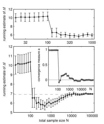
Figure 1: Displayed are free energy estimates $\widehat{\Delta f}$ in dependence of the sample size $N$, reaching a seemingly stable plateau if $N$ is restricted to $N=1000$ (top panel). Another stable plateau is reached if the sample size is increased up to $N=100\,000$ (bottom panel). Has the estimate finally converged? The answer is given by the corresponding graph of the convergence measure $a$ which is shown in the inset. The fluctuations around zero indicate convergence. The exact value of the free energy difference is visualized by the dashed horizontal line.

If we do not know whether the large $N$ limit is reached, we cannot state a reliable confidence interval of the free energy estimate: a problem which encounters frequently within free energy calculations is that the estimates “converge” towards a stable plateau. While the sample variance can become small, it remains unclear whether the reached plateau represents the correct value of $\Delta f$. Possibly, the found plateau is subject to some large bias, i.e. far off the correct value. A typical situation is displayed in Fig. 1 which shows successive two-sided free energy estimates in dependence of the sample size $N$. The errorbars are obtained with an error-propagation formula for the variance of $\widehat{\Delta f}$ which reflects the sample variances, see Appendix C after reading Sec. III. If we take a look on the top panel of Fig. 1, we might have the impression that the free energy estimate has converged at $N\approx 300$ already, while the bottom panel reaches out to larger sample sizes where it becomes visible that the “convergence” in the top panel was just pretended. Finally, we may ask if the estimates shown in the bottom panel have converged at $N\gtrsim 10000$? As we know the true value of $\Delta f$, which is depicted in the figure as a dashed line, we can conclude that convergence actually happened.

The main result of the present paper is the statement of a convergence criterion for two-sided free energy estimation in terms of the behavior of the convergence measure $a$. As will be seen, $a$ converges to zero. Moreover, this happens almost simultaneously with the convergence of $\widehat{\Delta f}$ to $\Delta f$. The procedure is as follows: While drawing an increasing number of work values in both directions (with fixed fraction $\alpha$ of forward draws), successive estimates $\widehat{\Delta f}$ and corresponding values of $a$, based on the present samples of work, are calculated. The values of $a$ are displayed graphically in dependence of $N$, preferably on a log-scale. Then the typical situation observed is that $a$ is close to it’s upper bound for small sample sizes $N<\frac{1}{\mathcal{A}}$, which indicates lack of “rare events” which are required in the averages of Eq. (2) (i.e. those events which “violate” the second law). Once $N$ becomes comparable to $\frac{1}{\mathcal{A}}$, single observations of rare events happen and change the value of $\widehat{\Delta f}$ and $a$ rapidly. In this regime of $N$, rare events are likely to be observed either disproportionally often or seldom, resulting in strong fluctuations of $a$ around zero. This indicates the transition region to the large $N$ limit. Finally, for some $N\gg\frac{1}{\mathcal{A}}$, the large $N$ limit is reached, and $a$ typically fluctuates close around zero, cf. the inset of Fig. 1.

The paper is organized as follows. In Sec. II, we first consider a simple model for the source of bias of two-sided estimation which is intended to obtain some insight into the convergence properties of two-sided estimation. The convergence measure $a$, which is introduced in Sec. III, however, will not depend on this specific model. As the convergence measure is based on a sample of forward and reverse work values, it is itself a random variable, raising the question of reliability once again. Using numerically simulated data, the statistical properties of the convergence measure will be elaborated in Sec. IV. The convergence criterion is stated in Sec. V, and Sec. VI presents an application to the estimation of the chemical potential of a Lennard-Jones fluid.

II Neglected tail model for two-sided estimation

To obtain some first qualitative insight into the relation between the convergence of Eq. (9) and the bias of the estimated free energy difference, we adopt the neglected tails model Wu2004 originally developed for one-sided free energy estimation.

Two-sided estimation of $\Delta f$ essentially means estimating the overlap $U_{\alpha}$ from two sides, however in a dependent manner, as $\widehat{\Delta f}$ is adjusted such that both estimates are equal in Eq. (9).

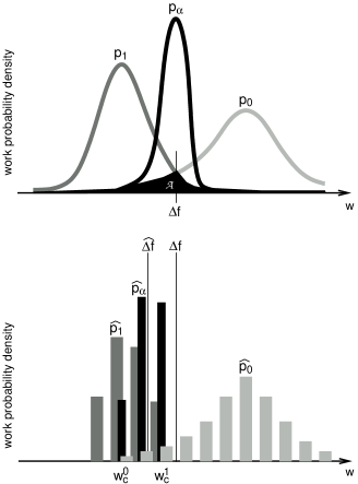
Figure 2: Schematic diagram of reverse $p_{1}$, overlap $p_{\alpha}$, and forward $p_{0}$ work densities (top). Schematic histograms of finite samples from $p_{0}$ and $p_{1}$, where in particular the latter is imperfectly sampled, resulting in a biased estimate $\widehat{\Delta f}$ of the free energy difference (bottom).

Consider the (normalized) overlap density $p_{\alpha}(w)$, defined as harmonic mean of $p_{0}$ and $p_{1}$:

$$p_{\alpha}(w)=\frac{1}{U_{\alpha}}\frac{p_{0}(w)p_{1}(w)}{\alpha p_{0}(w)+\beta p_{1}(w)}.$$ (11)

For $\alpha\to 0$ and $\alpha\to 1$, $p_{\alpha}$ converges to $p_{0}$ and $p_{1}$, respectively. The dominant contributions to $U_{\alpha}$ come from the overlap region of $p_{0}$ and $p_{1}$ where $p_{\alpha}$ has its main probability mass, see Fig. 2 (top).

In order to obtain an accurate estimate of $\Delta f$ with the two-sided estimator (2), the sample $\{w^{0}_{k}\}$ drawn from $p_{0}$ has to be representative for $p_{0}$ up to the overlap region in the left tail of $p_{0}$, and the sample $\{w^{1}_{k}\}$ drawn from $p_{1}$ has to be representative for $p_{1}$ up to the overlap region in the right tail of $p_{1}$. For small $n_{0}$ and $n_{1}$, however, we will have certain effective cut-off values $w^{0}_{c}$ and $w^{1}_{c}$ for the samples from $p_{0}$ and $p_{1}$, respectively, beyond which we typically will not find any work values, see Fig. 2 (bottom).

We introduce a model for the bias (4) of two-sided free energy estimation as follows. Assuming a “semi-large” $N=n_{0}+n_{1}$, the effective behavior of the estimator for fixed $n_{0}$ and $n_{1}$ is modeled by substituting the sample averages appearing in the estimator (2) with ensemble averages, however truncated at $w^{0}_{c}$ and $w^{1}_{c}$, respectively:

$$\int\limits_{w^{0}_{c}}^{\infty}\frac{p_{0}(w)}{\beta+\alpha e^{w-\left\langle\widehat{\Delta f}\right\rangle}}dw=\int\limits_{-\infty}^{w^{1}_{c}}\frac{p_{1}(w)}{\alpha+\beta e^{-w+\left\langle\widehat{\Delta f}\right\rangle}}dw.$$ (12)

Thereby, the cut-off values $w^{i}_{c}$ are thought fixed (only depending on $n_{0}$ and $n_{1}$) and the expectation $\left\langle\widehat{\Delta f}\right\rangle$ is understood to be the unique root of Eq. (12), thus being a function of the cut-off values $w^{i}_{c}$, $i=0,1$.

In order to elaborate the implications of this model, we rewrite Eq. (12) with the use of the fluctuation theorem (1) such that the integrands are equal,

$$e^{\left\langle\widehat{\Delta f}-\Delta f\right\rangle}=\frac{\int\limits_{-\infty}^{w^{1}_{c}}\frac{p_{0}(w)}{\alpha e^{w-\left\langle\widehat{\Delta f}\right\rangle}+\beta}dw}{\int\limits_{w^{0}_{c}}^{\infty}\frac{p_{0}(w)}{\alpha e^{w-\left\langle\widehat{\Delta f}\right\rangle}+\beta}dw},$$ (13)

and consider two special cases:

1. Large $n_{1}$ limit: Assume the sample size $n_{1}$ is large enough to ensure that the overlap region is fully and accurately sampled (large $n_{1}$ limit). Thus, $w^{1}_{c}$ can be safely set equal to $\infty$ in Eq. (13), and the r.h.s. becomes larger than unity. Accordingly, our model predicts a positive bias.

2. Large $n_{0}$ limit: Turning the tables and using $w^{0}_{c}=-\infty$ in Eq. (13), the model implies a negative bias.

In essence, $\left\langle\widehat{\Delta f}\right\rangle$ is shifted away from $\Delta f$ towards the insufficiently sampled density. In general, when none of the densities is sampled sufficiently, the bias will be a trade off between the two cases.

Qualitatively, from the neglected tails model, we find the main source of bias resulting from a different convergence behavior of forward and reverse estimates (9) of $U_{\alpha}$. The task of the next section will be to develop a quantitative measure of convergence.

III The convergence measure

In order to check convergence, we propose a measure which relies on a consistency check of estimates based on first and second moments of the Fermi functions that appear in the two-sided estimator (9). In a recent study Hahn2009a , we already used this measure for the special case of $\alpha=\frac{1}{2}$. Here, we give a generalization to arbitrary $\alpha$, study the convergence measure in greater detail, and justify its validity and usefulness. In the following we will assume that the densities $p_{0}$ and $p_{1}$ have the same support.

It was discussed in the preceding section that the large $N$ limit is reached and hence the bias of two-sided estimation vanishes if the overlap $U_{\alpha}$ is (in average) correctly estimated from both sides, $0$ and $1$. Defining the complementary Fermi functions $t_{c}(w)$ and $b_{c}(w)$ (for given $\alpha$) with

$$t_{c}(w)=\frac{1}{\alpha+\beta e^{-w+c}},$$

$$b_{c}(w)=\frac{1}{\alpha e^{w-c}+\beta},$$ (14)

such that $\alpha t_{c}(w)+\beta b_{c}(w)=1$ and $t_{c}(w)=e^{w-c}b_{c}(w)$ holds. The overlap (7) can be expressed in terms of first moments,

$$U_{\alpha}=\int t_{\scriptscriptstyle\Delta f}(w)p_{1}(w)dw=\int b_{\scriptscriptstyle\Delta f}(w)p_{0}(w)dw,$$ (15)

and the overlap estimate $\widehat{U}_{\alpha}$, Eq. (9), is simply obtained by replacing in Eq. (15) the ensemble averages by sample averages,

$$\widehat{U}_{\alpha}=\overline{t_{\scriptscriptstyle\widehat{\Delta f}}}^{\scriptscriptstyle(1)}=\overline{b_{\scriptscriptstyle\widehat{\Delta f}}}^{\scriptscriptstyle(0)}.$$ (16)

According to Eq. (2), the value of $\widehat{\Delta f}$ is defined such that the above relation holds. Note that $\widehat{\Delta f}=\widehat{\Delta f}(w^{0}_{1},\ldots,w^{1}_{n_{1}})$ is a single-valued function depending on all work values used in both directions. The overbar with index $(i)$ denotes an average with a sample $\{w^{i}_{k}\}$ drawn from $p_{i}$, $i=0,1$. For an arbitrary function $g(w)$ it explicitly reads

$$\overline{g}^{\scriptscriptstyle(i)}=\frac{1}{n_{i}}\sum\limits_{k=1}^{n_{i}}g(w^{i}_{k})$$ (17)

Interestingly, $U_{\alpha}$ can be expressed in terms of second moments of the Fermi functions such that it reads

$$U_{\alpha}=\alpha\int t_{\scriptscriptstyle\Delta f}^{2}p_{1}dw+\beta\int b_{\scriptscriptstyle\Delta f}^{2}p_{0}dw$$ (18)

A useful test of self-consistency is to compare the first order estimate $\widehat{U}_{\alpha}$, with the second order estimate $\widehat{U}^{\scriptscriptstyle(I\!I)}_{\alpha}$, where the latter is defined by replacing the ensemble averages in Eq. (18) with sample averages:

$$\widehat{U}^{\scriptscriptstyle(I\!I)}_{\alpha}=\alpha\overline{t_{\scriptscriptstyle\widehat{\Delta f}}^{2}}^{\scriptscriptstyle(1)}+\beta\overline{b_{\scriptscriptstyle\widehat{\Delta f}}^{2}}^{\scriptscriptstyle(0)}.$$ (19)

Thereby, the estimates $\widehat{\Delta f}$, $\widehat{U}_{\alpha}$, and $\widehat{U}^{\scriptscriptstyle(I\!I)}_{\alpha}$, are understood to be calculated with the same pair of samples $\{w^{0}_{k}\}$ and $\{w^{1}_{l}\}$.

The relative difference of this comparison results in the definition of the convergence measure,

$$a=\frac{\widehat{U}_{\alpha}-\widehat{U}^{\scriptscriptstyle(I\!I)}_{\alpha}}{\widehat{U}_{\alpha}},$$ (20)

for all $\alpha\in(0,1)$. Clearly, in the large $N$ limit, $a$ will converge to zero, as then $\widehat{\Delta f}$ converges to $\Delta f$ and thus $\widehat{U}_{\alpha}$ as well as $\widehat{U}^{\scriptscriptstyle(I\!I)}_{\alpha}$ converge to $U_{\alpha}$. As argued below, it is the estimate $\widehat{U}^{\scriptscriptstyle(I\!I)}_{\alpha}$ that converges last, hence $a$ converges somewhat later than $\widehat{\Delta f}$.

Below the large $N$ limit, $a$ will deviate from zero. From the general inequality

$$\widehat{U}_{\alpha}^{2}\leq\widehat{U}^{\scriptscriptstyle(I\!I)}_{\alpha}<2\widehat{U}_{\alpha}$$ (21)

(see Appendix B) follow upper and lower bounds on $a$ which read

$$-1<a\leq 1-\widehat{U}_{\alpha}<1.$$ (22)

The behavior of $a$ with increasing sample size $N=n_{0}+n_{1}$ (while keeping the fraction $\alpha=\frac{n_{0}}{N}$ constant) can roughly be characterized as follows: $a$ “starts” close to its upper bound for small $N$ and decreases towards zero with increasing $N$. Finally, $a$ begins to fluctuate around zero when the large $N$ limit is reached, i.e. when the estimate $\widehat{\Delta f}$ converges.

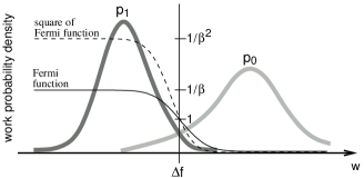
Figure 3: Schematic plot which shows that the forward work density, $p_{0}(w)$, samples the Fermi function $b_{\scriptscriptstyle\Delta f}(w)=1/(\beta+\alpha e^{w-\Delta f})$ somewhat earlier than its square.

To see this qualitatively, we state that the second order estimate $\widehat{U}^{\scriptscriptstyle(I\!I)}_{\alpha}$ converges later than the first order estimate $\widehat{U}_{\alpha}$, as the former requires sampling the tails of $p_{0}$ and $p_{1}$ to a somewhat wider extend than the latter, cf. Fig. 3. For small $N$, both, $\widehat{U}_{\alpha}$ and $\widehat{U}^{\scriptscriptstyle(I\!I)}_{\alpha}$, will typically underestimate $U_{\alpha}$, as the “rare-events” which contribute substantially to the averages (16) and (19) are quite likely not to be observed sufficiently, if at all. For the same reason, generically $\widehat{U}^{\scriptscriptstyle(I\!I)}_{\alpha}<\widehat{U}_{\alpha}$ will hold, since $b_{\scriptscriptstyle\widehat{\Delta f}}(w^{0})^{2}\leq b_{\scriptscriptstyle\widehat{\Delta f}}(w^{0})$ holds for $w^{0}\geq\widehat{\Delta f}$ and similar $t_{\scriptscriptstyle\widehat{\Delta f}}(w^{1})^{2}\leq t_{\scriptscriptstyle\widehat{\Delta f}}(w^{1})$ for $w^{1}\leq\widehat{\Delta f}$. Therefore, $a$ is typically positive for small $N$. In particular, if $N$ is so small that all work values of the forward sample are larger than $\widehat{\Delta f}$ and all work values of the reverse sample are smaller than $\widehat{\Delta f}$, then $\widehat{U}^{\scriptscriptstyle(I\!I)}_{\alpha}$ becomes much smaller than $\widehat{U}_{\alpha}$, resulting in $a\approx 1$.

Analytic insight into the behavior of $a$ for small $N$ results from the fact that $n\overline{x}^{2}\geq\overline{x^{2}}$ for any set $\{x_{1},\ldots x_{n}\}$ of positive numbers $x_{k}$. Using this in Eq. (19) yields

$$\widehat{U}^{\scriptscriptstyle(I\!I)}_{\alpha}\leq 2N\alpha\beta\widehat{U}_{\alpha}^{2}$$ (23)

and

$$1-2\alpha\beta N\widehat{U}_{\alpha}\leq a\leq 1-\widehat{U}_{\alpha}.$$ (24)

This shows that as long as $N\widehat{U}_{\alpha}\ll 1$ holds, $a$ is close to its upper bound $1-\widehat{U}_{\alpha}\approx 1$. In particular, if $\alpha=\frac{1}{2}$ and $N=2$, then $a=1-\widehat{U}_{\alpha}$ holds exactly.

Averaging the inequality for some $N$ sufficiently large to ensure $\left\langle a\right\rangle\approx 0$ and $\left\langle\widehat{U}_{\alpha}\right\rangle\approx U_{\alpha}$, we get a lower bound on $N$ which reads $N\geq\frac{1}{2\alpha\beta U_{\alpha}}$. Again, this bound can be related to the overlap area $\mathcal{A}$: taking $\alpha=\frac{1}{2}$ and using $U_{\frac{1}{2}}\leq 2\mathcal{A}$ (see Appendix A), we obtain $N\geq\frac{1}{\mathcal{A}}$, in concordance with the lower bound for the large $N$ limit stated in Sec. I.

Last we note that the convergence measure $a$ can also be understood as a measure of the sensibility of relation (2) with respect to the value of $\widehat{\Delta f}$: in the low $N$ regime, the relation is highly sensible to the value of $\widehat{\Delta f}$, resulting in large values of $a$, whereas in the limit of large $N$, relation (2) becomes insensible to small perturbations of $\widehat{\Delta f}$, corresponding to $a\approx 0$. The details are summarized in Appendix D.

IV Study of statistical properties of the convergence measure

Figure 4: Exponential (left panel) and Gaussian (right panel) work densities.

In order to demonstrate the validity of $a$ as a measure of convergence of two-sided free energy estimation, we apply it to two qualitatively different types of work densities, namely exponential and Gaussian, see Fig. 4. Samples from these densities are easily available by standard (pseudo) random generators. Statistical properties of $a$ are obtained by means of independent repeated calculations of $\widehat{\Delta f}$ and $a$. While the two types of densities used are fairly simple, they are entirely different and general enough to reflect the statistical properties of the convergence measure.

IV.1 Exponential work densities

The first example uses exponential work densities, i.e.

$$p_{i}(w)=\frac{1}{\mu_{i}}e^{-\frac{w}{\mu_{i}}},\quad w\geq 0,$$ (25)

$\mu_{i}>0$, $i=0,1$. According to the fluctuation theorem (1), the mean values $\mu_{i}$ of $p_{0}$ and $p_{1}$ are related to each other, $\mu_{1}=\frac{\mu_{0}}{1+\mu_{0}}$, and the free energy difference is known to be $\Delta f=\ln(1+\mu_{0})$.

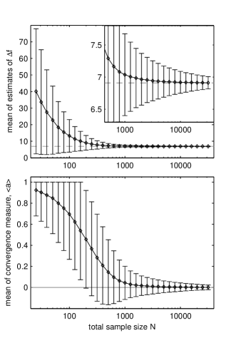
Figure 5: Statistics of two-sided free energy estimation (exponential work densities): shown are averaged estimates of $\Delta f$ in dependence of the total sample size $N$. The errorbars reflect the standard deviation. The dashed line shows the exact value of $\Delta f$, and the inset the details for large $N$ (top). Statistics of the convergence measure $a$ corresponding to the estimates of the top panel: shown are the average values of $a$ together with their standard deviation in dependence of the sample size $N$. Note the characteristic convergence of $a$ towards zero in the large $N$ limit (bottom).

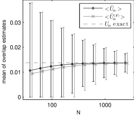
Figure 6: Mean values of overlap estimates $\widehat{U}_{\alpha}$ and $\widehat{U}^{\scriptscriptstyle(I\!I)}_{\alpha}$ of first and second order, respectively. The slightly slower convergence of $\widehat{U}^{\scriptscriptstyle(I\!I)}_{\alpha}$ towards $U_{\alpha}$ results in the characteristic properties of the convergence measure $a$. To enhance clarity, data points belonging to the same value of $N$ are spread.

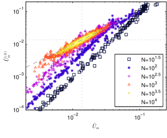
Figure 7: (Color online) Double-logarithmic scatter plot of $\widehat{U}^{\scriptscriptstyle(I\!I)}_{\alpha}$ versus $\widehat{U}_{\alpha}$ for many individual estimates in dependence of the sample size $N$. The dotted lines mark the exact value of $U_{\alpha}$ on the axes, and the dashed line is the bisectrix $\widehat{U}^{\scriptscriptstyle(I\!I)}_{\alpha}=\widehat{U}_{\alpha}$. The approximatively linear relation between the logarithms of $\widehat{U}^{\scriptscriptstyle(I\!I)}_{\alpha}$ and $\widehat{U}_{\alpha}$ is continued up to the smallest observed values ($<10^{-100}$, not shown here).

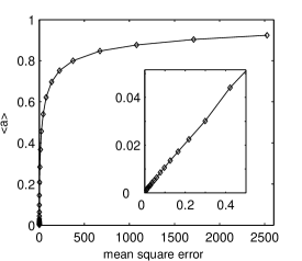
Figure 8: The average convergence measure $\left\langle a\right\rangle$ plotted against the corresponding mean square error $\left\langle(\widehat{\Delta f}-\Delta f)^{2}\right\rangle$ of the two-sided free energy estimator. The inset shows an enlargement for small values of $\left\langle a\right\rangle$.

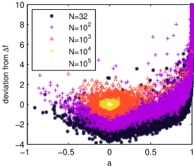
Figure 9: (Color online) A scatter plot of the deviation $\widehat{\Delta f}-\Delta f$ versus the convergence measure $a$ for many individual estimates in dependence of the sample size $N$. Note that the majority of estimates belonging to $N=32$ and $N=100$ have large values of $\widehat{\Delta f}-\Delta f$ well outside the displayed range with $a$ being close to one.

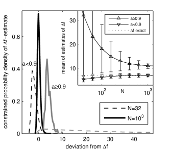
Figure 10: Estimated constrained probability densities $p(\widehat{\Delta f}|a\!<\!0.9)$ (black) and $p(\widehat{\Delta f}|a\!\geq\!0.9)$ (grayscale) for two different sample sizes $N$, plotted versus the deviation $\widehat{\Delta f}-\Delta f$. The inset shows averaged estimates of $\Delta f$ over the total sample size $N$ subject to the constraints $a\geq 0.9$ and $a<0.9$, respectively.

Choosing $\mu_{0}=1000$ and $\alpha=\frac{1}{2}$, i.e. $n_{0}=n_{1}$, we calculate free energy estimates $\widehat{\Delta f}$ according to Eq. (2) together with the corresponding values of $a$ according to Eq. (20) for different total sample sizes $N=n_{0}+n_{1}$. An example of a single running estimate and the corresponding values of the convergence measure are depicted in Fig. 1. Ten-thousand repetitions for each value of $N$ yield the results presented in Figs. 5–10. To begin with, the top panel of Fig. 5 shows the averaged free energy estimates in dependence of $N$, where the errorbars show $\pm$ the estimated square root of the variance $\left\langle(\widehat{\Delta f}-\langle\widehat{\Delta f}\rangle)^{2}\right\rangle$. For small $N$, the bias $\left\langle\widehat{\Delta f}-\Delta f\right\rangle$ of free energy estimates is large, but becomes negligible compared to the standard deviation for $N\gtrsim 5000$. This is a prerequisite of the large $N$ limit, therefore we will view $N\approx 5000$ as the onset of the large $N$ limit.

The bottom panel of Fig. 5 shows the averaged values of the convergence measure $a$ corresponding to the free energy estimates of the top panel. Again, the errorbars are $\pm$ one standard deviation $\sqrt{\left\langle a^{2}\right\rangle-\left\langle a\right\rangle^{2}}$, except that the upper limit is truncated for small $N$, as $a<1$ holds. The trend of the averaged convergence measure $\left\langle a\right\rangle$ is in full agreement with the general considerations given in the previous section: for small $N$, $\left\langle a\right\rangle$ starts close to its upper bound, decreases monotonically with increasing sample size, and converges towards zero in the large $N$ limit. At the same time, its standard deviation converges to zero, too. This indicates that single values of $a$ corresponding to single estimates $\widehat{\Delta f}$ will typically be found close to zero in the large $N$ regime.

Noting that $a$ is defined as relative difference of the overlap estimators $\widehat{U}_{\alpha}$ and $\widehat{U}^{\scriptscriptstyle(I\!I)}_{\alpha}$ of first and second order, respectively, we can understand the trend of the average convergence measure by taking into consideration the average values $\left\langle\widehat{U}_{\alpha}\right\rangle$ and $\left\langle\widehat{U}^{\scriptscriptstyle(I\!I)}_{\alpha}\right\rangle$, which are shown in Fig. 6. For small sample sizes, $U_{\alpha}$ is typically underestimated by both, $\widehat{U}_{\alpha}$ and $\widehat{U}^{\scriptscriptstyle(I\!I)}_{\alpha}$, with $\widehat{U}^{\scriptscriptstyle(I\!I)}_{\alpha}<\widehat{U}_{\alpha}$.

The convergence measure takes advantage of the different convergence times of the overlap estimators: $\widehat{U}^{\scriptscriptstyle(I\!I)}_{\alpha}$ converges somewhat slower than $\widehat{U}_{\alpha}$, ensuring that $a$ approaches zero right after $\widehat{\Delta f}$ has converged. The large standard deviations shown as errorbars in Fig. 6 do not carry over to the standard deviation of $a$, because $\widehat{U}_{\alpha}$ and $\widehat{U}^{\scriptscriptstyle(I\!I)}_{\alpha}$ are strongly correlated, as is impressively visible in Fig. 7. The estimated correlation coefficient

$$\frac{\left\langle\big{(}\widehat{U}^{\scriptscriptstyle(I\!I)}_{\alpha}-\langle\widehat{U}^{\scriptscriptstyle(I\!I)}_{\alpha}\rangle\big{)}\big{(}\widehat{U}_{\alpha}-\langle\widehat{U}_{\alpha}\rangle\big{)}\right\rangle}{\sqrt{\operatorname{Var}\big{(}\widehat{U}^{\scriptscriptstyle(I\!I)}_{\alpha}\big{)}\operatorname{Var}\big{(}\widehat{U}_{\alpha}\big{)}}}$$ (26)

is about $0.97$ (!) for the entire range of sample sizes $N$. In good approximation, $\widehat{U}_{\alpha}$ and $\widehat{U}^{\scriptscriptstyle(I\!I)}_{\alpha}$ are related to each other according to a power law, $\widehat{U}^{\scriptscriptstyle(I\!I)}_{\alpha}\approx c_{N}\widehat{U}_{\alpha}^{\ \gamma_{N}}$, where the exponent $\gamma_{N}$ and the prefactor $c_{N}$ depend on the sample size $N$ (and $\alpha$). We note that $\gamma_{N}$ has a phase-transition-like behavior: for small $N$, it stays approximately constant near two; right before the onset of the large $N$ limit, it shows a sudden switch to a value close to one where it finally remains.

Figure 8 accents the decrease of the average $\left\langle a\right\rangle$ with decreasing mean square error (5) of two-sided estimation. The small $N$ behavior is given by the upper right part of the graph, where $\left\langle a\right\rangle$ is close to its upper bound together with a large mean square error of $\widehat{\Delta f}$. With increasing sample size, the mean square error starts to drop somewhat sooner than $\left\langle a\right\rangle$, however, at the onset of the large $N$ limit, they drop both and suggest a linear relation, as can be seen in the inset for small values of $\left\langle a\right\rangle$. The latter shows that $\left\langle a\right\rangle$ decreases to zero proportional to $\frac{1}{N}$ for large $N$ (this is confirmed by a direct check, but not shown here).

The next point is to clarify the correlation of single values of the convergence measure with their corresponding free energy estimates. For this issue, figure 9 is most informative, showing the deviations $\widehat{\Delta f}-\Delta f$ in dependence of the corresponding values of $a$ for many individual observations. The figure makes clear that there is a strong relation, but no one-to-one correspondence between $a$ and $\widehat{\Delta f}-\Delta f$: For large $N$, both $a$ and $\widehat{\Delta f}-\Delta f$ approach zero with very weak correlations between them. However, the situation is different for small sample sizes $N$ where the bias $\left\langle\widehat{\Delta f}-\Delta f\right\rangle$ is considerably large. There, the typically observed large deviations occur together with values of $a$ close to the upper bound, whereas the atypical events with small (negative) deviations come together with values of $a$ well below the upper limit. Therefore, small values of $a$ detect exceptional events if $N$ is well below the large $N$ limit, and ordinary events if $N$ is large.

To make this relation more visible, we split the estimates $\widehat{\Delta f}$ into the mutually exclusive events $a\geq 0.9$ and $a<0.9$. The statistics of the $\widehat{\Delta f}$ values within these cases are depicted in the inset of Fig. 10, where normalized histograms, i.e. estimates of the constrained probability densities $p(\widehat{\Delta f}|a\!\geq\!0.9)$ and $p(\widehat{\Delta f}|a\!<\!0.9)$ are shown. The unconstrained probability density of $\widehat{\Delta f}$ can be reconstructed from a likelihood weighted sum of the constrained densities, $p(\widehat{\Delta f})=p(\widehat{\Delta f}|a\!\geq\!0.9)p_{\scriptscriptstyle a\geq 0.9}+p(\widehat{\Delta f}|a\!<\!0.9)p_{\scriptscriptstyle a<0.9}$. The likelihood ratios read $p_{\scriptscriptstyle a\geq 0.9}/p_{\scriptscriptstyle a<0.9}=6.2$ and $0.002$ for $N=32$ and $1000$, respectively. Finally, the inset of Fig. 10 shows the average values of constrained estimates $\widehat{\Delta f}$ over $N$ with errorbars of $\pm$ one standard deviation, in dependence of the condition on $a$.

IV.2 Gaussian work densities

For the second example the work-densities are chosen to be Gaussian,

$$p_{i}(w)=\frac{1}{\sigma\sqrt{2\pi}}e^{-\frac{(w-\mu_{i})^{2}}{2\sigma^{2}}},\quad w\in\mathds{R},$$ (27)

$i=0,1$. The fluctuation theorem (1) demands both densities to have the same variance $\sigma^{2}$ with mean values $\mu_{0}=\Delta f+\frac{1}{2}\sigma^{2}$ and $\mu_{1}=\Delta f-\frac{1}{2}\sigma^{2}$. Hence, $p_{0}$ and $p_{1}$ are symmetric to each other with respect to $\Delta f$, $p_{0}(\Delta f+w)=p_{1}(\Delta f-w)$. As a consequence of this symmetry, the two-sided estimator with equal sample sizes $n_{0}$ and $n_{1}$, i.e. $\alpha=0.5$, is unbiased for any $N$. However, this does not mean that the limit of large $N$ is reached immediately.

In analogy to the previous example, we proceed in presenting the statistical properties of $a$. Choosing $\sigma=6$ and without loss of generality $\Delta f=0$, we carry out $10^{4}$ estimations of $\Delta f$ over a range of sample sizes $N$. The forward fraction is chosen to be equal to $\alpha=0.5$, and for comparison, $\alpha=0.999$, and $\alpha=0.99999$, respectively. In the latter two cases, the two-sided estimator is biased for small $N$. We note that $\alpha=0.5$ is always the optimal choice for symmetric work densities which minimizes the asymptotic mean square error (6) with respect to $\alpha$ Hahn2009b .

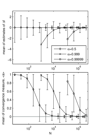
Figure 11: Gaussian work densities result in the displayed averaged estimates of $\Delta f$. For comparison, three different fractions $\alpha$ of forward work values are used (top). Average values of the convergence measure $a$ corresponding to the estimates of the top panel (bottom).

Comparing the top and the bottom panel of Fig. 11, which show the statistics (mean value and standard deviation as errorbars) of the observed estimates $\widehat{\Delta f}$ and of the corresponding values of $a$, we find a coherent behavior for all three cases of $\alpha$ values. The trend of the average $\left\langle a\right\rangle$ shows in all cases the same features in agreement with the trend found for exponential work densities.

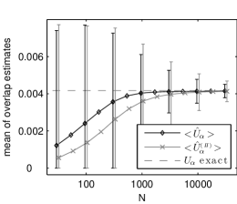
Figure 12: Mean values of overlap estimates $\widehat{U}_{\alpha}$ and $\widehat{U}^{\scriptscriptstyle(I\!I)}_{\alpha}$ of first and second order ($\alpha=0.5$).

As before, the characteristics of $a$ are understood by the slower convergence of $\widehat{U}^{\scriptscriptstyle(I\!I)}_{\alpha}$ compared to that of $\widehat{U}_{\alpha}$, as can be seen in Fig. 12. A scatter plot of $\widehat{U}^{\scriptscriptstyle(I\!I)}_{\alpha}$ versus $\widehat{U}_{\alpha}$ looks qualitatively like Fig. 7, but is not shown here.

Figure 13: The average convergence measure $\left\langle a\right\rangle$ plotted against the corresponding mean square error $\left\langle(\widehat{\Delta f}-\Delta f)^{2}\right\rangle$ of free energy estimates in dependence of $N$.

Figure 13 compares the average convergence measures as functions of the mean square error of $\widehat{\Delta f}$ for the three values of $\alpha$. For the range of small $\left\langle a\right\rangle$, all three curves agree and are linear. Again $\left\langle a\right\rangle$ decreases proportionally to $\frac{1}{N}$ for large $N$. Noticeable for small $N$ is the shift of $\left\langle a\right\rangle$ towards smaller values with increasing $\alpha$. This results from the definition of $a$: the upper bound $1-\widehat{U}_{\alpha}$ of $a$ tends to zero in the limits $\alpha\to 0,1$, as then $\widehat{U}_{\alpha}\to 1$.

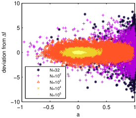
Figure 14: (Color online) A scatter plot of the deviation $\widehat{\Delta f}-\Delta f$ versus the convergence measure $a$ for many individual estimates in dependence of the sample size $N$ ($\alpha=0.5$).

The relation of single free energy estimates $\widehat{\Delta f}$ with the corresponding $a$ values can be seen in the scatter plot of Fig. 14. The mirror symmetry of the plot originates from the symmetry of the work densities and the choice $\alpha=0.5$, i.e. of the unbiasedness of the two-sided estimator. Opposed to the foregoing example, the correlation between $\widehat{\Delta f}-\Delta f$ and $a$ vanishes for any value of $N$. Despite the lack of any correlation, the figure reveals a strong relation between the deviation $\widehat{\Delta f}-\Delta f$ and the value of $a$: they converge equally to zero for large $N$.

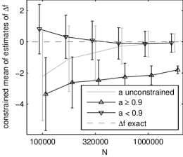
Figure 15: Averaged two-sided estimates of $\Delta f$ in dependence of the total sample size $N$ for the constraints $a\geq 0.9$, $a$ unconstrained, and $a<0.9$ ($\alpha=0.99999$).

Last, figure 15 shows averages of constrained $\Delta f$ estimates for the mutually exclusive conditions $a\geq 0.9$ and $a<0.9$, now with $\alpha=0.99999$ in order to incorporate some bias. We observe the same characteristics as before, cf. the inset of Fig. 10: The condition $a<0.9$ filters the estimates $\widehat{\Delta f}$ which are closer to the true value.

IV.3 The general case

The characteristics of the convergence measure are dominated by contributions of work densities inside and near the region where the overlap density $p_{\alpha}(w)$, Eq. (11), has most of its mass. We call this region the overlap region. In the overlap region, the work densities may have one of the following characteristic relation of shape:

1. Having their maxima at larger and smaller values of work, respectively, the forward and reverse work densities both drop towards the overlap region. Hence, any of both densities sample the overlap region by rare events, only, which are responsible for the behavior of the convergence measure.

2. Both densities decrease with increasing $w$ and the overlap region is well sampled by the forward work density compared with the reverse density. Especially the “rare” events $w<\Delta f$ of forward direction are much more available than the rare events $w>\Delta f$ of reverse direction. Hence, more or less typical events of one direction together with atypical events of the other direction are responsible for the behavior of the convergence measure. Likewise if both densities increase with $w$.

3. More generally, the work densities are some kind of interpolation between the above two cases.

4. Finally, there remain some exceptional cases. For instance, if the forward and reverse work densities have different support or if they do not obey the fluctuation theorem at all.

With respect to the exceptional case, the convergence measure fails to work, since it requires that the forward and reverse work densities have the same support and that the densities are related to each other via the fluctuation theorem (1).

In all other cases, the convergence measure certainly will work and will show a similar behavior, regardless of the detailed nature of the densities. This can be explained as follows. In the preceding subsections, we have investigated exponential and Gaussian work densities, two examples that differ in their very nature. While exponential work densities cover case number two, and Gaussians cover case number one, they show the same characteristics of $a$. This means that the characteristics of the convergence measure are insensitive to the individual nature of the work densities as long as they have the same support and obey the fluctuation theorem.

To this end, we want to point to some subtleties in the text of the actual paper. While the measure of convergence is robust with respect to the nature of work densities, some heuristic or pedagogic explanations in the text are written with regard to the typical case number one, where the overlap region is sampled by rare events, only. This concerns mainly Sec. II where we speak about effective cut-off values in the context of the neglected tail model. These effective cut-off values would become void if we would try to explain the bias of exponential work densities qualitatively via the neglected tail model. Also the explanations in the text of the next section are mainly focused on the typical case number one. This concerns the passages where we speak about rare events. Nevertheless, the main and essential statements are valid for all cases.

The most important property of $a$ is its almost simultaneous convergence with the free energy estimator $\widehat{\Delta f}$ to an à priori known value. This fact is used to develop a convergence criterion in the next section.

V The convergence criterion

Elaborated the statistical properties of the convergence measure, we are finally interested in the convergence of a single free energy estimate. In contrast to averages of many independent running estimates, estimates based on individual realization are not smooth in $N$, see e.g. Fig. 1.

For small $N$, typically $\widehat{U}^{\scriptscriptstyle(I\!I)}_{\alpha}$ underestimates $U_{\alpha}$ more than $\widehat{U}_{\alpha}$ does, pushing $a$ close to its upper bound. With increasing $N$, $\widehat{\Delta f}$ starts to “converge”; typically in a non-smooth manner. The convergence of $\widehat{\Delta f}$ is triggered by the occurrence of rare events. Whenever such a rare event in the important tails of the work densities gets sampled, $\widehat{\Delta f}$ jumps, and between such jumps, $\widehat{\Delta f}$ stays rather on a stable plateau. The measure $a$ is triggered by the same rare events, but the changes in $a$ are smaller, unless convergence starts happening. Typically, the rare events that bring $\widehat{\Delta f}$ near to its true value are the rare events which change the value of $a$ drastically. In the typical case, these rare events let $a$ even undershoot below zero, before $\widehat{\Delta f}$ and $a$ finally converge.

The features of the convergence measure,

1. it is bounded, $a\in(-1,\,1-\widehat{U}_{\alpha}]$,

2. it starts for small $N$ at its upper bound,

3. it converges to a known value, $a\to 0$,

4. and typically it converges almost simultaneously with $\widehat{\Delta f}$,

simplify the task of monitoring the convergence significantly, since it is far easier to compare estimates of $a$ with the known value zero than the task of monitoring convergence of $\widehat{\Delta f}$ to an unknown target value. The characteristics of the convergence measure enable us to state: typically, if a is close to zero, $\widehat{\Delta f}$ has converged.

Deviations from the typical situation are possible. For instance, $\widehat{\Delta f}$ may not show such clear jumps, neither may $a$. Occasionally, $\widehat{\Delta f}$ and $a$, may also fluctuate exceedingly strong. Thus, a single value of $a$ close to zero does not guarantee convergence of the free energy estimate as can be seen from some few individual events in the scatter plot of Fig. 14 that fail a correct estimate while $a$ is close to zero. A single random realization may give rise to a fluctuation that brings $a$ close to zero by chance, a fact that needs to be distinguished from $a$ having converged to zero. The difference between random chance and convergence is revealed by increasing the sample size, since it is highly unlikely that $a$ stays close to zero by random. It is the behavior of $a$ with increasing $N$, that needs to be taken into account in order to establish an equivalence between $a\to 0$ and $\widehat{\Delta f}\to\Delta f$.

This allows us to state the convergence criterion:

• if $a$ fluctuates close around zero, convergence is assured,

implying that if $a$ fluctuates around zero, $\widehat{\Delta f}$ fluctuates around its true value $\Delta f$, the bias vanishes, and the mean square error reaches its asymptotics which can be estimated using Eq. (8). $a$ fluctuating close around zero means that it does so over a suitable range of sample sizes, which extends over an order of magnitude or more.

VI Application

As an example, we apply the convergence criterion to the calculation of the excess chemical potential $\mu^{ex}$ of a Lennard Jones fluid. Using Metropolis Monte Carlo simulation Metropolis1953 of a fluid of $N_{p}$ particles, the forward work is defined as energy increase when inserting at random a particle into a given configuration Widom1963 , whereas the reverse work is defined as energy decrease when a random particle is deleted from a given $N_{p}+1$-particle configuration. The densities $p_{0}(w)$ and $p_{1}(w)$ of forward and reverse work obey the fluctuation theorem (1) with $\Delta f=\mu^{ex}$ Hahn2009a . Thus, Bennett’s acceptance ratio method can be applied to the calculation of the chemical potential.

Details of the simulation are reported in Ref. Hahn2009a . Here, the parameter values chosen read: $N_{p}=120$, reduced Temperature $T^{*}=1.2$, and reduced density $\rho^{*}=0.5$.

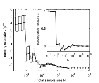
Figure 16: Running estimates of the excess chemical potential $\mu^{ex}$ in dependence of the sample size $N$ ($\alpha=0.9$). The inset displays the corresponding values of the convergence measure $a$.

Drawing work values up to a total sample size of $10^{6}$ with fraction $\alpha=0.9$ of forward draws (which will be a near-optimal choice Hahn2009b ), the successive estimates of the chemical potential together with the corresponding values of the convergence measure are shown in Fig. 16. The dashed horizontal line does not show the exact value of $\mu^{ex}$, which is unknown, but rather the value of the last estimate with $N=10^{6}$. Taking a closer look on the behavior of the convergence measure with increasing $N$, we observe $a$ near unity for $N\leq 10^{2}$, indicating the low $N$ regime and the lack of observing rare events. Then, a sudden drop near to zero happens at $N=10^{2}$, which coincides with a large jump of the estimate of $\mu^{ex}$, followed by large fluctuations of $a$ with strong negative values in the regime $N=10^{2}$ to $10^{4}$. This behavior indicates that the important but rare events which trigger the convergence of the $\mu^{ex}$ estimate are now sampled, but with strongly fluctuating relative frequency, which in specific cases causes the negative values of $a$ (because of too many rare events!). Finally, with $N>10^{4}$, $a$ equilibrates and converges to zero. The latter is observed over two orders of magnitude, such that we can conclude that the latest estimate of $\mu^{ex}$ with $N=10^{6}$ has surely converged and yields a reliable value of the chemical potential. The confidence interval of the estimate can safely be calculated as the square root of Eq. (6) (one standard deviation), and we obtain explicitly $\widehat{\mu^{ex}}=-2.451\pm 0.005$.

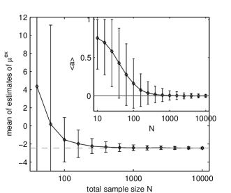
Figure 17: Statistics of estimates of the excess chemical potential: shown are the average value and the standard deviation (as errorbars) in dependence of the sample size $N$. The statistics of the corresponding values of the convergence measure is shown in the inset.

Interested in the statistical behavior of $a$ for the present application, we carried out 270 simulation runs up to $N=10^{4}$ to obtain the average values and standard deviations of $\widehat{\mu^{ex}}$ and $a$ which are depicted in Fig. 17. The dashed line marks the same value as that in Fig. 16. Again, we observe the same qualitative behavior of $a$ as in the foregoing examples of Sec. V, especially a positive average value of $\left\langle a\right\rangle$ and a convergence to zero which occurs simultaneously with the convergence of Bennett’s acceptance ratio method.

VII Conclusions

Since its formulation a decade ago, the Jarzynski equation and the Crooks fluctuation theorem gave rise to enforced research of nonequilibrium techniques for free energy calculations. Despite the variety of new methods, in general little is known about their statistical properties. In particular, it is often unclear whether the methods actually converge to the desired value of the free energy difference $\Delta f$, and if so, it remains in question whether convergence happened within a given calculation. This is of great concern, as usually the calculations are strongly biased before convergence starts happening. In consequence, it is impossible to state the result of a single calculation of $\Delta f$ with a reliable confidence interval unless a convergence measure is evaluated.

In this paper, we presented and tested a quantitative measure of convergence for two-sided free energy estimation, i.e. Bennett’s acceptance ratio method, which is intimately related to the fluctuation theorem. From this follows a criterion for convergence relying on monitoring the convergence measure $a$ within a running estimation of $\Delta f$. The heart of the convergence criterion is the nearly simultaneous convergence of the free energy calculation and the convergence measure $a$. Whereas the former converges towards the unknown value $\Delta f$, which makes it difficult or even impossible to decide when convergence actually takes place, the latter converges to an à priori known value. If convergence is detected with the convergence criterion, the calculation results in a reliable estimate of the free energy difference together with a precise confidence interval.

Appendix A

The derivation of inequality (10) relies on the close connection between the overlap $U_{\alpha}$ and the overlap area $\mathcal{A}$,

$$U_{\alpha}=\int\frac{p_{0}p_{1}}{\alpha p_{0}+\beta p_{1}}dw\geq\int\frac{p_{0}p_{1}}{(\alpha+\beta)\max\{p_{0},p_{1}\}}dw=\int\min\{p_{0},p_{1}\}dw=\mathcal{A},$$ (28)

$$U_{\frac{1}{2}}=2\int\frac{1}{1/p_{1}+1/p_{0}}dw<2\int\min\{p_{0},p_{1}\}dw=2\mathcal{A}.$$ (29)

Together with the inequality $\frac{1}{2}X(N,\frac{1}{2})\leq X(N,\alpha)$ of Bennett Bennett1976 , we obtain

$$\frac{1-2\mathcal{A}}{N\mathcal{A}}<\frac{1-U_{\frac{1}{2}}}{\frac{1}{2}NU_{\frac{1}{2}}}=\frac{1}{2}X(N,\frac{1}{2})\leq X(N,\alpha)\leq\frac{1}{N}\frac{1}{\alpha\beta}\big{(}\frac{1}{\mathcal{A}}-1\big{)}$$ (30)

which directly yields inequality (10).

Appendix B

Inequality (21) can be obtained as follows. Noting that $t_{c}(w)<\frac{1}{\alpha}$ and $b_{c}(w)<\frac{1}{\beta}$, cf. Eqs. (14) we have

$$2\widehat{U}_{\alpha}=\overline{t_{\scriptscriptstyle\widehat{\Delta f}}}^{\scriptscriptstyle(1)}+\overline{b_{\scriptscriptstyle\widehat{\Delta f}}}^{\scriptscriptstyle(0)}>\alpha\overline{t_{\scriptscriptstyle\widehat{\Delta f}}^{2}}^{\scriptscriptstyle(1)}+\beta\overline{b_{\scriptscriptstyle\widehat{\Delta f}}^{2}}^{\scriptscriptstyle(0)}=\widehat{U}^{\scriptscriptstyle(I\!I)}_{\alpha}\qquad\qquad\text{and further}$$ (31)

$$\widehat{U}^{\scriptscriptstyle(I\!I)}_{\alpha}=\widehat{U}_{\alpha}^{2}+\alpha\overline{(t_{\scriptscriptstyle\widehat{\Delta f}}-\widehat{U}_{\alpha})^{2}}^{\scriptscriptstyle(1)}+\beta\overline{(b_{\scriptscriptstyle\widehat{\Delta f}}-\widehat{U}_{\alpha})^{2}}^{\scriptscriptstyle(0)}\geq\widehat{U}_{\alpha}^{2},$$ (32)

which results in Eq. (21).

Appendix C

The errorbars in Figs. 1 and 16 are obtained via the error-propagation formula for the variance of Bennett’s acceptance ratio method.

A possible estimate $\widehat{\sigma}_{ep}^{2}$ of the variance of the two-sided free energy estimator obtained from error-propagation reads

$$\widehat{\sigma}_{ep}^{2}=\frac{1}{n_{1}}\frac{\overline{t_{\scriptscriptstyle\widehat{\Delta f}}^{2}}^{\scriptscriptstyle(1)}-{\overline{t_{\scriptscriptstyle\widehat{\Delta f}}}^{\scriptscriptstyle(1)}}^{2}}{{\overline{t_{\scriptscriptstyle\widehat{\Delta f}}}^{\scriptscriptstyle(1)}}^{2}}+\frac{1}{n_{0}}\frac{\overline{b_{\scriptscriptstyle\widehat{\Delta f}}^{2}}^{\scriptscriptstyle(0)}-{\overline{b_{\scriptscriptstyle\widehat{\Delta f}}}^{\scriptscriptstyle(0)}}^{2}}{{\overline{b_{\scriptscriptstyle\widehat{\Delta f}}}^{\scriptscriptstyle(0)}}^{2}}$$ (33)

Alternatively, $\widehat{\sigma}_{ep}^{2}$ can be expressed through the overlap estimates $\widehat{U}_{\alpha}$ and $\widehat{U}^{\scriptscriptstyle(I\!I)}_{\alpha}$ of first and second order, Eqs. (16) and (19),

$$\widehat{\sigma}_{ep}^{2}=\frac{1}{\alpha\beta N}\frac{\widehat{U}^{\scriptscriptstyle(I\!I)}_{\alpha}-\widehat{U}_{\alpha}^{2}}{\widehat{U}_{\alpha}^{2}}.$$ (34)

In the limit of large $N$, $\widehat{\sigma}_{ep}^{2}$ converges to the asymptotic mean square error $X(N,\alpha)$, Eq. (6). An upper bound on $\widehat{\sigma}_{ep}^{2}$ follows from inequality (23):

$$\widehat{\sigma}_{ep}^{2}\leq 2-\frac{1}{\alpha\beta N}.$$ (35)

Finally let us mention that the convergence measure $a$, Eq. (20), is closely related to the relative difference of the estimated asymptotic mean square error $\hat{X}$, Eq. (8), and $\widehat{\sigma}_{ep}^{2}$:

$$a=(1-\widehat{U}_{\alpha})\frac{\hat{X}-\widehat{\sigma}_{ep}^{2}}{\hat{X}}.$$ (36)

Appendix D

Consider the family $\widehat{\phi}(c)$ of $\Delta f$ estimators, parametrized by the real number $c$ Bennett1976 :

$$\widehat{\phi}(c)=c+\ln\frac{\overline{t_{c}}^{\scriptscriptstyle(1)}}{\overline{b_{c}}^{\scriptscriptstyle(0)}}.$$ (37)

For any fixed value of $c$, $\widehat{\phi}(c)$ defines a consistent estimator of $\Delta f$, $\widehat{\phi}(c)\overset{N\to\infty}{\longrightarrow}\Delta f\quad\forall c$. For finite $N$, however, the performance of the estimator strongly depends on $c$. The (optimal) two-sided estimate (2) is obtained by the additional condition $\widehat{\phi}(c)=c$, such that $\overline{t_{c}}^{\scriptscriptstyle(1)}=\overline{b_{c}}^{\scriptscriptstyle(0)}$ holds, and thus $c=\widehat{\Delta f}$. A possible measure for the sensibility of the estimate $\widehat{\phi}(c)$ on $c$ is it’s derivative with respect to $c$. Using $\frac{\partial}{\partial c}t_{c}=-\beta t_{c}b_{c}$, $\frac{\partial}{\partial c}b_{c}=\alpha t_{c}b_{c}$, and $\alpha t_{c}+\beta b_{c}=1$, we obtain

$$\frac{\partial}{\partial c}\widehat{\phi}(c)=-1+\alpha\frac{\overline{t_{c}^{2}}^{\scriptscriptstyle(1)}}{\overline{t_{c}}^{\scriptscriptstyle(1)}}+\beta\frac{\overline{b_{c}^{2}}^{\scriptscriptstyle(0)}}{\overline{b_{c}}^{\scriptscriptstyle(0)}}.$$ (38)

Taking the derivative at $c=\widehat{\Delta f}$ directly results in the convergence measure $a$,

$$\frac{\partial}{\partial c}\widehat{\phi}(c)|_{\widehat{\Delta f}}=-a.$$ (39)

References

- (1) J. G. Kirkwood, J. Chem. Phys. 3, 300 (1935).
- (2) A. Gelman and X.-L. Meng, Stat. Science. 13, 163 (1998).
- (3) D. D. L. Minh and J. D. Chodera, J. Chem. Phys. 131, 134110 (2009).
- (4) R. W. Zwanzig, J. Chem. Phys. 22, 1420 (1954).
- (5) G. M. Torrie and J. P. Valleau, J. Comput. Phys. 23, 187 (1977).
- (6) M.-H. Chen and Q.-M. Shao, Annals of Stat. 25, 1563 (1997).
- (7) H. Oberhofer and C. Dellago, Comput. Phys. Comm. 179, 41 (2008).
- (8) M. Watanabe and W. P. Reinhardt, Phys. Rev. Lett. 65, 3301 (1990).
- (9) S. X. Sun, J. Chem. Phys. 118, 5769 (2003).
- (10) F. M. Ytreberg and D. M. Zuckerman, J. Chem. Phys. 120, 10876 (2004).
- (11) C. Jarzynski, Phys. Rev E 73, 046105 (2006).
- (12) H. Ahlers and A. Engel, Eur. Phys. J. B 62, 357 (2008).
- (13) H. Then and A. Engel, Phys. Rev. E 77, 041105 (2008).
- (14) P. Geiger and C. Dellago, Optimum protocol for fast-switching free-energy calculations, accepted for publication in Phys. Rev. E (2010).
- (15) A. Engel, Phys. Rev. E 80, 021120 (2009).
- (16) X.-L. Meng and S. Schilling, J. Comput. Graph. Stat. 11, 552 (2002).
- (17) C. Jarzynski, Phys. Rev. E 65, 046122 (2002).
- (18) H. Oberhofer, C. Dellago, and S. Boresch, Phys. Rev. E 75, 061106 (2007).
- (19) S. Vaikuntanathan and C. Jarzynski, Phys. Rev. Lett. 100, 190601 (2008).
- (20) A. M. Hahn and H. Then, Phys. Rev. E 79, 011113 (2009).
- (21) N. Lu and T. B. Woolf, in Ch. Chipot and A. Pohorille (eds.), Free Energy Calculations, Springer Series in Chem. Phys. 86, Springer Berlin, 2007, pp. 199–247.
- (22) P. Maragakis, F. Ritort, C. Bustamante, M. Karplus, and G. E. Crooks, J. Chem. Phys. 129, 024102 (2004).
- (23) C. H. Bennett, J. Comput. Phys. 22, 245 (1976).
- (24) X.-L. Meng and W. H. Wong, Stat. Sin. 6, 831 (1996).
- (25) A. Kong, P. McCullagh, X.-L. Meng, D. Nicolae, and Z. Tan, J. R. Stat. Soc. B 65, 585 (2003).
- (26) M. R. Shirts and J. D. Chodera, J. Chem. Phys. 129, 124105 (2008).
- (27) G. E. Crooks, Phys. Rev. E 60, 2721 (1999).
- (28) M. Campisi, P. Talkner, and P. Hänggi, Phys. Rev. Lett. 102, 210401 (2009).
- (29) C. Jarzynski, Phys. Rev. Lett. 78, 2690 (1997).
- (30) G. E. Crooks, Phys. Rev. E 61, 2361 (2000).
- (31) M. R. Shirts, E. Bair, G. Hooker, and V. S. Pande, Phys. Rev. Lett. 91, 140601 (2003).
- (32) A. M. Hahn and H. Then, Phys. Rev. E 80, 031111 (2009).
- (33) D. Wu and D. A. Kofke, J. Chem. Phys. 121, 8742 (2004).
- (34) N. Metropolis, A. W. Rosenbluth, M. N. Rosenbluth, A. H. Teller, and E. Teller, J. Chem. Phys. 21, 1087 (1953).
- (35) B. Widom, J. Chem. Phys. 39, 2808 (1963).