FISH: A 3D parallel MHD code for astrophysical applications

Abstract

fish is a fast and simple ideal magneto-hydrodynamics code that scales to $\sim 10\,000$ processes for a Cartesian computational domain of $\sim 1000^{3}$ cells. The simplicity offish has been achieved by the rigorous application of the operator splitting technique, while second order accuracy is maintained by the symmetric ordering of the operators. Between directional sweeps, the three-dimensional data is rotated in memory so that the sweep is always performed in a cache-efficient way along the direction of contiguous memory. Hence, the code only requires a one-dimensional description of the conservation equations to be solved. This approach also enable an elegant novel parallelisation of the code that is based on persistent communications with MPI for cubic domain decomposition on machines with distributed memory. This scheme is then combined with an additional OpenMP parallelisation of different sweeps that can take advantage of clusters of shared memory. We document the detailed implementation of a second order TVD advection scheme based on flux reconstruction. The magnetic fields are evolved by a constrained transport scheme. We show that the subtraction of a simple estimate of the hydrostatic gradient from the total gradients can significantly reduce the dissipation of the advection scheme in simulations of gravitationally bound hydrostatic objects. Through its simplicity and efficiency, fish is as well-suited for hydrodynamics classes as for large-scale astrophysical simulations on high-performance computer clusters. In preparation for the release of a public version, we demonstrate the performance of fish in a suite of astrophysically orientated test cases.

1 Introduction

It has been argued that computational models provide the third pillar of scientific discovery, beside the traditional experiment and theory. On the practical side, there are indeed a lot of similarities between computer models and experiments: In both cases one tries to start from a well-defined initial state. The outcome of the simulation is in the same way unknown as the outcome of an experiment and unexpected results are interesting in both cases. Also, one has to define observables whose values one intends to measure at several time intervals or at the end of the simulation or experiment. If the computer model or experiment is complicated enough, these values will be affected by systematic and statistical errors and their understanding requires an involved theoretical analysis and interpretation. Finally, both computer model and experiment need sufficient, and sometimes quite extensive, documentation to make the results reproducible.

On the other hand, only the real experiment is capable of probing the properties of nature, while the computer model is bound to elaborate the properties of the theory it is built on. The strength of the computer simulation is that it may demonstrate and extend the predictive power of its underlying theory. In principle, though, it seems completely irrelevant whether the consequences of the underlying theory are evaluated by analytical approaches or a computer-aided model. The computer model can be regarded as the analytical evolution of a discretised model of the physics equations, where the computer only provides appreciated efficiency in the evaluations, but does not add anything new to an analytical investigation.

This leads to our point of view that the computer model is not an independent pillar of science, but an increasingly important contemporary method in the development of theory. The computer model is most helpful if many different physics aspects are intertwined in a manner that prevents the treatment of the problem by dividing it into subproblems. Classical examples are found in research areas whose subject is inaccessible to human manipulation and preparation in the laboratory, like meteorology, planetary interiors, stars, and astrophysical dynamics in general.

Because physics on many different length and time scales is involved, it is of primary importance to first perform order of magnitude estimates to identify irrelevant processes and to find equilibrium conditions that constrain degrees of freedom. A classical theoretical model is then built by the description of a sequence of dominant processes, supported by order of magnitude estimates. The next step in the traditional approach is to approximate the complicated microscopic input physics by simple analytical fitting formulas that depend on few parameters. If the fitting formulas are simple enough, the problem might become analytically solvable so that the dependence of the global features on the chosen parameters can be revealed. In stellar structure, for example, order of magnitude arguments show that the matter is in thermodynamical equilibrium. Hence, an equation of state can be defined that expresses the gas pressure, $p$, as a function of the local density, $\rho$, temperature and composition. In some regimes, the microscopic physics information in the equation of state is well approximated by an equation of state of the form $p=\kappa\rho^{1+1/n}$. Here, $\kappa$ is a constant and $n$ a parameter called the polytropic index. If this approximation holds, the equations of stellar structure can be integrated analytically for selected integer values of $n$ [1, 2]. Hence, traditional theoretical astrophysics relies on two prongs: (1) the interpretation of observations in terms of scenarios that are supported by order of magnitude estimates, and (2) the explanation of complicated processes by simple approximate laws that allow a precise analytical investigation of the most important aspects of the model.

It is obvious how scientific computing can extend the lever of approach (2). As soon as the complicated processes are reduced to simple approximate laws, the initial state and the equations of evolution of the model are mathematically well-defined. It is therefore possible to replace the former analytical investigation by calculations on the computer. For example, the Lane-Emden equation can be integrated numerically for many more values of the polytropic index. There is only one mathematically correct answer to each problem and the numerical calculation can be refined until the algorithm obtains the desired precision of the result.

It is much more intricate to let computer models contribute to approach (1), i.e. the interpretation of observations in terms of scenarios that are supported by order of magnitude estimates. A well-known example is the propagation of a shock front. Only a minority of computer codes attempt to resolve the microscopic width of the shock to correctly treat its complicated input physics. Most codes just ensure the accurate conservation of mass, momentum and energy across the shock front to obtain the shock propagation speed and the thermodynamic conditions on both sides of the shock. Here, it is the numerical algorithm that dynamically performs the simplification of the model and not the description of the input physics like in approach (2). Hence, one may implement a rich set of input physics and design the finite differencing such that fundamental laws of physics are fulfilled under all possible conditions. Then, the complexity of the model is bound by the scale on which unresolvable small-scale structures are dissipated in space and time. Because this scale depends on the numerical algorithm and the mesh topology rather than the investigated physics, different solutions of the same physics problem may not converge to the same microscopic solution. However, the goal of approach (1) is not to evaluate the detailed microscopic state of $\sim 10^{9}$ individual fluid cells (for a human being it would take several years of uninterrupted reading to absorb this amount of information), but to elaborate the generic macroscopic properties that are determined by the fundamental physics laws in combination with the microscopic input physics. The actual microscopic state of the fluid cells acts as an exemplary sampling of a specific macroscopic state. Convergence of the evolution of the macroscopic state must be demonstrated by careful comparison and theoretical interpretation of concurrent implementations of the same physics problem using different algorithms and meshes. Hence, we believe that it is important for the reliability of astrophysical models to be investigated with several different radiation-magneto-hydrodynamics codes that are simple and efficient enough to be broadly used.

There are several well-documented and publicly available software packages. gadget is a cosmological N-body code based on the Smoothed Particle Hydrodynamics method and parallelised using the Message Passing Interface (MPI). It is a Lagrangean approach with a hierarchical tree for the non-local evaluation of Newtonian gravity [3]. vh-1 is a multidimensional hydrodynamics code based on the Lagrangian remap version of the Piecewise Parabolic Method (PPM) [4] that has been further developed and parallelised using MPI. zeus-2D [5, 6, 7] and zeus-3D are widely used grid-based hydrodynamics codes for which a MPI-parallel zeus-mp version exists as well. It offers the choice of different advection schemes on a fixed or moving orthogonal Eulerian mesh in a covariant description. While these more traditional approaches distribute in the form of a software package that includes options to switch on or off, recent open source projects try to provide the codes in the form of a generic framework that can host a variety of different modules implementing different techniques. In this category we could mention the flash code [8, 9] with its main focus on the coupling of adaptive mesh stellar hydrodynamics to nuclear burning and the whisky code [10] as a recent general relativistic hydrodynamics code based on the cactus environment. Further we mention athena [11] and enzo [12] which are both well documented and publicly available codes.

In this paper we present our code fish (Fast and Simple Ideal magneto-Hydrodynamics), which follows a somewhat different strategy. fish is based on the publicly available serial version of a cosmological hydrodynamics code [13]. Its main virtue is the simplicity and the straightforward approach on a Cartesian mesh. It can equally well be used for educational purpose in hydrodynamics classes than for three-dimensional high-resolution astrophysical simulations [14]. However, in the first code versions, simplicity and parallel efficiency were not available at the same time. Here we describe a new and elegant implementation of the parallelisation with a hybrid MPI/OpenMP approach that has been redesigned from scratch and is well separated from the subroutines describing the physical conservation equations. Hence, the same code version is now simple and efficient on large high-performance computing clusters. In comparison to the above-mentioned software packages it is simple to modify and/or extend and has negligible overhead. With respect to earlier versions, the discretisation of the advection terms and the implementation of gravity has further been developed to make the fish code more accurate in the treatment of fast cold flows and more stable for the evolution of gravitationally bound hydrostatic objects. Special attention was given to the robustness of the approach in regions with poor resolution, which are difficult to avoid in global astrophysical models. fish has successfully been used in one of the first predictions of the gravitational wave signal from 3D supernova models with microscopic input physics [15] and provides the foundation for the implementation of spectral neutrino transport in our new code elephant (ELegant and Efficient Parallel Hydrodynamics with Approximate Neutrino Transport) [16].

In Section 2 we describe the physics equations and document the numerical methods used in fish. In Section 3 we discuss the optimisation of the memory access, the parallelisation of fish with MPI and OpenMP and present the scaling behaviour to $\sim 10000$ processes. In Section 4 we finally investigate the performance of fish in a suit of six mostly magneto-hydrodynamic test problems.

2 Numerical methods

Solving the MHD equations numerically involves overcoming at least two challenges. Firstly the difficulty of solving the Riemann problem, used as building blocks for Godunov type shock capturing numerical schemes, due to the non-strict hyperbolicity of the MHD equations, see e.g. [17, 18, 19]. The second problem is the divergenceless constraint on the magnetic field. A non-vanishing divergence of the magnetic field can produce an acceleration of the magnetised fluid parallel to the field lines [20].

The algorithm of Pen et al. [13] solves the first problem by using a Riemann solver free relaxation method [21]. The second issue is addressed by using a constrained transport method [22] on a staggered grid.

The algorithm of Pen et al. makes extensive use of operator splitting. In particular, the evolution of the conducting fluid and the magnetic field are split by first holding the magnetic field constant and evolving the fluid and then performing the reverse action. The source terms arising due to gravity are also accounted for in the operator splitting method. Further, the full three dimensional problem is dimensionally split into one-dimensional subproblems. An adequately ordered application of the solution operators permits second order accuracy in time [23].

2.1 The equations of ideal magnetohydrodynamics

The equations of ideal magnetohydrodynamics (MHD) describe the movement of a compressible conducting fluid subject to magnetic fields. In ideal MHD all dissipative processes are neglected, meaning that the fluid possesses no viscosity and its conductivity is assumed to be infinite. The ideal MHD equations then read [24]

$$\frac{\partial\rho}{\partial t}+\nabla\cdot\left(\rho\boldsymbol{v}\right) = 0$$ (1)

$$\frac{\partial\rho\boldsymbol{v}}{\partial t}+\nabla\cdot\left(\boldsymbol{v}\rho\boldsymbol{v}-\boldsymbol{b}\boldsymbol{b}\right)+\nabla P_{tot} = -\rho\nabla\phi$$ (2)

$$\frac{\partial E}{\partial t}+\nabla\cdot\left[\left(E+P_{tot}\right)\boldsymbol{v}-\boldsymbol{b}\left(\boldsymbol{v}\cdot\boldsymbol{b}\right)\right] = -\rho\boldsymbol{v}\cdot\nabla\phi$$ (3)

$$\frac{\partial\boldsymbol{b}}{\partial t}-\nabla\times\left(\boldsymbol{v}\times\boldsymbol{b}\right) = 0,$$ (4)

expressing the conservation of mass, momentum, energy and magnetic flux, respectively. Here $\rho$ is the mass density, $\boldsymbol{v}$ the velocity and $E=\rho e+\frac{\rho}{2}v^{2}+\frac{b^{2}}{2}$ the total energy being, the sum of internal, kinetic and magnetic energy. The magnetic field is given by $\boldsymbol{B}=/\sqrt{4\pi}\boldsymbol{b}$ and $P_{tot}=p+\frac{b^{2}}{2}$ is the total pressure, being the sum of the gas pressure and the magnetic pressure. For the equation of state we assume an ideal gas law

$$p=\rho e(\gamma-1)$$ (5)

where $\gamma$ is the ratio of specific heats. The right hand side of the momentum and energy conservation equations detail the effect of gravitational forces onto the conserved variables. The gravitational potential $\phi$ is determined by the Poisson equation

$$\nabla^{2}\phi=4\pi\rho.$$ (6)

The MHD equations (1-4) conserve the divergence of the magnetic field so that an initial condition

$$\nabla\cdot\boldsymbol{b}=0$$ (7)

remains true, consistent with the physical observation that magnetic monopoles have never been observed.

Before we start describing the individual solution operators, we first introduce our notation. We discretise time into discrete steps $\Delta t^{n}$ and space into finite volumes or cells $V_{i,j,k}$ where $n$ labels the different time levels and the triple $(i,j,k)$ denotes a particular cell. The vector $\boldsymbol{u}=\left(\rho,\rho v_{x},\rho v_{y},\rho v_{z},E\right)^{T}$ denotes the conserved fluid variables. The solution vector $\boldsymbol{u}^{n}_{i,j,k}$ contains the spatially averaged values of the conserved variables at time $t$ in cell $V_{i,j,k}$

$$\boldsymbol{u}_{i,j,k}=\frac{1}{V_{i,j,k}}\int_{V_{i,j,k}}\boldsymbol{u}\left(\boldsymbol{x},t\right)\mathrm{d}x\mathrm{d}y\mathrm{d}z,$$ (8)

where the cell volume $V_{i,j,k}=\Delta x\Delta y\Delta z$ is given by the assumed constant cell dimensions $\Delta x=x_{i^{\prime}}-x_{i^{\prime}-1}$, $\Delta y=y_{j^{\prime}}-y_{j^{\prime}-1}$, $\Delta z=z_{k^{\prime}}-z_{k^{\prime}-1}$. Half-integer indices are indicated by a prime $i^{\prime}=i+1/2$, $j^{\prime}=j+1/2$, $k^{\prime}=k+1/2$ and denote the intercell boundary. Further we define the cell face averaged magnetic field components at time $t$ by

$$\left(b_{x}\right)_{i^{\prime},j,k}=\frac{1}{S_{i^{\prime},j,k}}\int_{S_{i^{\prime},j,k}}b_{x}\left(\boldsymbol{x},t\right)\mathrm{d}y\mathrm{d}z$$ (9)

$$\left(b_{y}\right)_{i,j^{\prime},k}=\frac{1}{S_{i,j^{\prime},k}}\int_{S_{i,j^{\prime},k}}b_{y}\left(\boldsymbol{x},t\right)\mathrm{d}x\mathrm{d}z$$ (10)

$$\left(b_{z}\right)_{i,j,k^{\prime}}=\frac{1}{S_{i,j,k^{\prime}}}\int_{S_{i,j,k^{\prime}}}b_{z}\left(\boldsymbol{x},t\right)\mathrm{d}x\mathrm{d}y$$ (11)

where $S_{i^{\prime},j,k}=\Delta y\Delta z$ denotes the cell face of cell $V_{i,j,k}$ located at $x_{i^{\prime}}$ and spanned by the zone increments $\Delta y$ and $\Delta z$. $\left(b_{y}\right)^{n}_{i,j^{\prime},k}$ and $\left(b_{z}\right)^{n}_{i,j,k^{\prime}}$ are defined analogously.

In an operator-split scheme the solution algorithm to the ideal MHD equations can be summarized as

$$\boldsymbol{u}^{n+2}=L_{\mathrm{forward}}L_{\mathrm{backward}}\boldsymbol{u}^{n},$$ (12)

where

$$L_{\mathrm{forward}} =L_{x}\left(\Delta t\right)B^{yz}_{x}\left(\Delta t\right)L_{y}\left(\Delta t\right)B^{xz}_{y}\left(\Delta t\right)L_{z}\left(\Delta t\right)B^{xy}_{z}\left(\Delta t\right)$$ (13)

$$L_{\mathrm{backward}} =L_{z}\left(\Delta t\right)B^{xy}_{z}\left(\Delta t\right)L_{y}\left(\Delta t\right)B^{xz}_{y}\left(\Delta t\right)L_{x}\left(\Delta t\right)B^{yz}_{x}\left(\Delta t\right)$$

are the forward and backward operator for one time step. The operators $L_{x,y,z}$ evolve the fluid and account for the source terms, while the $B$ operators evolve the magnetic field. If the individual operators are second order accurate, then the application of the forward followed by the backward operator is second order accurate in time [23]. In the following subsections we shall detail the individual operators.

The numerical solution algorithm to the MHD equations is explicit. Hence we are restricted by the Courant, Friedrich and Lewy [25] (CFL) condition. Therefore we impose the following time step

$$\Delta t^{n}=k\cdot\min_{i,j,k}\left(\frac{\Delta x}{C_{i,j,k}^{n,x}},\frac{\Delta y}{C_{i,j,k}^{n,y}},\frac{\Delta z}{C_{i,j,k}^{n,z}}\right)$$ (14)

where

$$C_{i,j,k}^{n,d}=\max\left(v_{d,i,j,k}^{n}+c_{Fi,j,k}^{n}\right)$$ (15)

is the maximum speed at which information can travel in the whole computational domain in direction $d=x,y,z$ being the sum of the velocity component in d and the speed of the fast magnetosonic waves $c_{F}$. We typically set the CFL number $k$ to $0.75$.

2.2 Solving the fluid MHD equations

In this subsection we describe the evolution of the fluid variables $\boldsymbol{u}$ in the $x$-direction. During this process the magnetic field is held constant and interpolated to cell centers. The gravitational source terms are assumed to vanish for the moment. Then mass, momentum and energy conservation in $x$ direction can be written as

$$\frac{\partial\boldsymbol{u}}{\partial t}+\frac{\partial\boldsymbol{F}}{\partial x}=0$$ (16)

where

$$\boldsymbol{F}=\left[\begin{array}[]{c}\rho v_{x}\\ \rho v_{x}^{2}+P_{tot}-b_{x}^{2}\\ \rho v_{x}v_{y}-b_{x}b_{y}\\ \rho v_{x}v_{z}-b_{x}b_{z}\\ (E+P_{tot})v_{x}-b_{x}\boldsymbol{b}\cdot\boldsymbol{v}\end{array}\right]$$ (17)

is the flux vector.

Integrating eq. (16) over a cell $V_{i,j,k}$ gives

$$\frac{\partial\boldsymbol{u}_{i,j,k}}{\partial t}+\frac{1}{\Delta x}\left(\boldsymbol{F}_{i^{\prime},j,k}-\boldsymbol{F}_{i^{\prime}-1,j,k}\right)=0$$ (18)

where the definition of the cell averaged values (8) has been substituted and Gauss’ theorem has been used. The numerical flux $\boldsymbol{F}_{i^{\prime},j,k}$ represents an average flux of the conserved quantities through the surface $S_{i^{\prime},j,k}$

$$\boldsymbol{F}_{i^{\prime},j,k}=\frac{1}{S_{i^{\prime},j,k}}\int_{S_{i^{\prime},j,k}}\boldsymbol{F}\left(\boldsymbol{x},t\right)\mathrm{d}y\mathrm{d}z$$ (19)

at given time $t$. Eq. (18) is a semi-discrete conservative scheme for the conservation law (16). In the following we focus on obtaining the numerical fluxes in a stable and accurate manner. Time integration of the ordinary differential equation (18) will be addressed later in this subsection.

Many schemes for the stable and accurate computation of the numerical fluxes have been devised in the literature. Godunov type methods achieve this by solving either exact or approximate Riemann problems at cell interfaces [26, 27, 28]. Through solving the Riemann problem, these methods ensure an upwind discretisation of the conservation law and hence achieve causal consistency. Due to the already mentioned difficulty of solving the Riemann problem in the ideal MHD case, the algorithm of Pen at el. [13] uses the relaxation scheme of Jin and Xin [21]. For detailed information on these type of methods we refer to [21, 29] and the references therein.

The idea of the relaxation scheme is to replace a system like (17) by a larger system

$$\frac{\partial\boldsymbol{u}}{\partial t}+\frac{\partial\boldsymbol{w}}{\partial x} =0$$ (20)

$$\frac{\partial\boldsymbol{w}}{\partial t}+D^{2}\frac{\partial\boldsymbol{u}}{\partial x} =\frac{1}{\epsilon}\left(\boldsymbol{F}(\boldsymbol{u})-\boldsymbol{w}\right),$$

called the relaxation system. Here, the relaxation rate $\epsilon$ is a small positive parameter and $D^{2}$ is a positive definite matrix. For small relaxation rates, system (20) rapidly relaxes to the local equilibrium defined by $\boldsymbol{w}=\boldsymbol{F}(\boldsymbol{u})$. A necessary condition for solutions of the relaxation system (20) to converge in the small $\epsilon$ limit to solutions of the original system (16) is that the characteristic speeds of the hyperbolic part of (20) are at least as large or larger than the characteristic speeds in system (16). This is the so-called subcharacteristic condition.

As in Ref. [21] we choose $D=d\cdot I$ to be a diagonal matrix. In order to fulfill the subcharacteristic condition the diagonal element $d$ or the so-called freezing speed is chosen to be

$$d=|v_{x}|+c_{F},$$ (21)

where $c_{F}$ is the speed of the fast magnetosonic waves, i.e. the fastest wave propagation speed supported by the equations of ideal MHD.

The key point in the relaxation system is that in the local equilibrium limit it has a very simple characteristic structure

$$\frac{\partial}{\partial t}\left(\boldsymbol{w}+D\boldsymbol{u}\right)+D\frac{\partial}{\partial x}\left(\boldsymbol{w}+D\boldsymbol{u}\right)=0$$ (22)

$$\frac{\partial}{\partial t}\left(\boldsymbol{w}-D\boldsymbol{u}\right)-D\frac{\partial}{\partial x}\left(\boldsymbol{w}-D\boldsymbol{u}\right)=0,$$

where $\boldsymbol{w}\pm D\boldsymbol{u}$ are then the characteristic variables. They travel with the “frozen” characteristic speeds $\pm D$ respectively.

System (22) can be easily recast into an equation for $\boldsymbol{u}$ and $\boldsymbol{w}$. However, we are practically only interested in that for $\boldsymbol{u}$

$$\frac{\partial\boldsymbol{u}}{\partial t}+\frac{\partial\boldsymbol{F^{+}}}{\partial x}+\frac{\partial\boldsymbol{F^{-}}}{\partial x}=0$$ (23)

where $\boldsymbol{F}^{+}=(\boldsymbol{w}+D\boldsymbol{u})/2$ denotes the right travelling waves and $\boldsymbol{F}^{-}=(\boldsymbol{w}-D\boldsymbol{u})/2$ the left travelling waves. In the follwing we shall drop the indices of the ignored directions. Since this defines an upwind direction for each wave component, a first order upwind scheme results from choosing $\boldsymbol{F}^{+}_{i^{\prime}}=\boldsymbol{F}^{+}_{i}$ and $\boldsymbol{F}^{-}_{i^{\prime}}=\boldsymbol{F}^{-}_{i+1}$. In this case, the total flux at the cell interfaces is readily evaluated to become

$$\boldsymbol{F}_{i^{\prime}}=\boldsymbol{F}^{+}_{i^{\prime}}+\boldsymbol{F}^{-}_{i^{\prime}}=\frac{1}{2}\left(\boldsymbol{F}_{i}+\boldsymbol{F}_{i+1}\right)-\frac{1}{2}D\left(\boldsymbol{u}_{i+1}-\boldsymbol{u}_{i}\right)$$ (24)

where $\boldsymbol{F}_{i}=\boldsymbol{w}_{i}=\boldsymbol{F}(\boldsymbol{u}_{i})$. For $D$ we use the freezing speed

$$d=\max\left(d_{i},d_{i+1}\right)$$ (25)

in order to satisfy the subcharacteristic condition. We note that this choice for the freezing speed makes the numerical flux equivalent to the Rusanov flux and the local Lax-Friedrichs flux. As pointed out in [29], a wide variety of numerical flux assignments can be derived from the relaxation system by simply letting the matrix $D$ having a more complicated form than diagonal.

So far, the numerical flux (24) is only first order accurate. First order methods permit the automatic capturing of flow discontinuities but are inaccurate in smooth flow regions due to the large amount of numerical dissipation inherent to them. As a matter of fact, the large numerical dissipation present in first order methods is not a deficit of theses methods but it is the reason why they are stable at flow discontinuities in the first place. However, in many applications both smooth and discontinuous flow features are present and therefore the use of higher order methods is desirable. We opt for a second order accurate total variation diminishing (TVD) scheme due to the low computational cost and the robustness of these type of schemes.

Let us first consider the right traveling waves $\boldsymbol{F}^{+}$. Given the $i$th cell, a first order accurate flux at the cell boundary $x_{i^{\prime}}$ is then given by $\boldsymbol{F}^{+}_{i^{\prime}}=\boldsymbol{F}^{+}_{i}=\boldsymbol{F}^{+}(\boldsymbol{u}_{i})$. This corresponds to a piece-wise constant approximation of the flux function $\boldsymbol{F}^{+}(x,t)$ over the staggered cell $[x_{i},x_{i+1}]$. For second order accuracy we seek a piece-wise linear approximation

$$\boldsymbol{F}^{+}(x,t)\approx\boldsymbol{F}^{+}_{i}+\left.\frac{\partial\boldsymbol{F}^{+}}{\partial x}\right|_{i}(x-x_{i})$$ (26)

where the derivative may be approximated from first order flux differences. Two choices exist: either left or right differences

$$\left.\frac{\partial\boldsymbol{F}^{+}}{\partial x}\right|_{i}=\left\{\begin{array}[]{l l l}\Delta\boldsymbol{F}^{+,L}_{i}=\left(\boldsymbol{F}^{+}_{i}-\boldsymbol{F}^{+}_{i-1}\right)/\Delta x\\ \\ \Delta\boldsymbol{F}^{+,R}_{i}=\left(\boldsymbol{F}^{+}_{i+1}-\boldsymbol{F}^{+}_{i}\right)/\Delta x\\ \end{array}\right..$$ (27)

To choose between the left $\Delta\boldsymbol{F}^{+,L}_{i}$ and right $\Delta\boldsymbol{F}^{+,R}_{i}$ differences a flux limiter $\phi$

$$\Delta\boldsymbol{F}^{+}_{i}=\phi\left(\Delta\boldsymbol{F}^{+,L}_{i},\Delta\boldsymbol{F}^{+,R}_{i}\right)$$ (28)

is used.

This limiter enforces a nonlinear stability constraint commonly known as TVD to ensure the stability of the scheme in the vicinity of discontinuities. The limiter reduces spurious oscillations associated with higher accuracy than first order to get a high resolution method. See for example [27, 30, 18, 28] and references therein.

We have implemented the minmod limiter

$$\phi(a,b)=\mathrm{minmod}(a,b)=\frac{1}{2}\left(\mathrm{sign}(a)+\mathrm{sign}(b)\right)\min(|a|,|b|)$$ (29)

which chooses the smallest absolute difference if both have the same sign, and the Van Leer limiter

$$\phi(a,b)=\frac{1}{2}\left(\mathrm{sign}(a)+\mathrm{sign}(b)\right)\frac{2ab}{a+b}.$$ (30)

Other choices are possible for the scheme to be TVD [21]. Note that when the left and right flux differences have different signs, i.e. at extrema and hence also at shocks, no correction is added in (26) and the scheme switches to first order accuracy. For core-collapse simulations we use the Van Leer limiter in the subsonic flow regions and the minmod limiter in supersonic regions.

In a similar way we may construct a piece-wise linear approximation for the left going fluxes $\boldsymbol{F}^{-}$ in the staggered cell $[x_{i},x_{i+1}]$ starting at $x_{i+1}$

$$\boldsymbol{F}^{-}(x,t)\approx\boldsymbol{F}^{-}_{i+1}+\left.\frac{\partial\boldsymbol{F}^{-}}{\partial x}\right|_{i+1}(x-x_{i+1})$$ (31)

with either the left or right differences

$$\left.\frac{\partial\boldsymbol{F}^{-}}{\partial x}\right|_{i+1}=\left\{\begin{array}[]{l l l}\Delta\boldsymbol{F}^{-,L}_{i+1}=\left(\boldsymbol{F}^{-}_{i+1}-\boldsymbol{F}^{-}_{i}\right)/\Delta x\\ \\ \Delta\boldsymbol{F}^{-,R}_{i+1}=\left(\boldsymbol{F}^{-}_{i+2}-\boldsymbol{F}^{-}_{i+1}\right)/\Delta x\\ \end{array}\right..$$ (32)

Again the flux limiter $\phi$ is used to discriminate between the left or right differences

$$\Delta\boldsymbol{F}^{-}_{i+1}=\phi\left(\Delta\boldsymbol{F}^{-,L}_{i+1},\Delta\boldsymbol{F}^{-,R}_{i+1}\right).$$ (33)

The total second order accurate numerical flux is then simply

$$\boldsymbol{F}_{i^{\prime}}=\boldsymbol{F}^{+}_{i}+\boldsymbol{F}^{-}_{i+1}+\frac{\Delta x}{2}\left(\Delta\boldsymbol{F}^{+}_{i}-\Delta\boldsymbol{F}^{-}_{i+1}\right).$$ (34)

For the time integration of eq. (18) we use a two step predictor-corrector method. As predictor we compute a half time step with the first order fluxes (24). We regard the freezing speed in the predictor step as a parameter varying between $d=0$ and $d=\max\left(d_{i},d_{i+1}\right)$ to regulate the numerical dissipation. Hence we vary the predictor between a first order scheme and a second order centered difference scheme depending on the application.

In the corrector step we then use the calculated values from the predictor step $\boldsymbol{u}^{n^{\prime}}$ to compute the second order TVD fluxes eq. (34):

$$\boldsymbol{u}_{i}^{n+1}=\boldsymbol{u}_{i}^{n}-\frac{\Delta t}{\Delta x}\left(\boldsymbol{F}_{i^{\prime}}^{n^{\prime}}-\boldsymbol{F}_{i^{\prime}-1}^{n^{\prime}}\right).$$ (35)

Hence we obtain a second order update in time and space of the fluid variables. This ends the description of the $L_{x}$ solution operator. The other spatial directions are treated in the same way.

2.3 Incorporation of gravitation

Gravitational forces play an important role in most astrophysical processes. A code devoted to the simulation of these processes should therefore include gravity and we describe our implementation in the following subsection. To integrate the source terms, we split the source term dimensionally as follows:

$$\frac{\partial\boldsymbol{u}}{\partial t}+\frac{\partial\boldsymbol{F}}{\partial x}=\boldsymbol{S}_{x}$$ (36)

where $\boldsymbol{S}_{x}=(0,-\rho\partial\phi/\partial x,0,0,-\rho v_{x}\partial\phi/\partial x)$, and in an analogous manner for the $y$ and $z$ direction. In the following we shall regard the gravitational potential as given and constant in time. For the integration of eq. (36) one then has two possibilities, either an operator split or an unsplit method.

In the fully operator split version, the evolution of the conserved variables is divided into a homogeneous system ($\boldsymbol{S}_{x}=0$) and the ordinary differential equation

$$\frac{\mathrm{d}\boldsymbol{u}}{\mathrm{d}t}=\boldsymbol{S}_{x}$$ (37)

Solving the homogeneous part has been discussed in the previous section. In operator notation, we then solve equation (36) as

$$\boldsymbol{u}^{n+1}=G_{x}\left(\frac{\Delta t}{2}\right)L_{x}\left(\Delta t\right)G_{x}\left(\frac{\Delta t}{2}\right)$$ (38)

which is second order accurate in time.

Further, for reasons to be explained in section 3, our code has as fundamental variables density, momentum and internal energy. Therefore we only update the momentum field, and the operator $G_{x}$ is then explicitly

$$G_{x}\left(\Delta t\right):\;(\rho\boldsymbol{v})_{i}^{n+1}=(\rho\boldsymbol{v})_{i}^{n}-\Delta t\cdot\rho_{i}^{n}\left(\frac{\partial\phi}{\partial x}\right)_{i}^{n},$$ (39)

where we use centered differences for the gravitational potential

$$\left(\frac{\partial\phi}{\partial x}\right)_{i}^{n}=\frac{\phi_{i+1}^{n}-\phi_{i-1}^{n}}{2\Delta x}.$$ (40)

Note that the density field is left constant according to (37). The total energy is computed by summing up internal energy, magnetic energy and kinetic energy and given as input to the $L_{x}$ operator. Therefore the total energy change due to the source term is implied from the updated momentum field.

As a second possibility, we implemented an unsplit version. There we directly account for gravity in the fluid predictor/corrector steps. The predictor step then is given by

$$\boldsymbol{u}_{i}^{n^{\prime}}=\boldsymbol{u}_{i}^{n}-\frac{\Delta t}{2\Delta x}\left(\boldsymbol{F}_{i^{\prime}}^{n}-\boldsymbol{F}_{i^{\prime}-1}^{n}\right)+\frac{\Delta t}{2}\boldsymbol{S}_{i}^{n}$$ (41)

where the $\boldsymbol{F}_{i^{\prime}}^{n}$ is the predictor flux as described in previous section and

$$\begin{aligned} \boldsymbol{S}_{i}^{n}=\left[\begin{array}[]{c}0\\ \rho_{i}^{n}\\ 0\\ 0\\ (\rho v_{x})_{i}^{n}\\ \end{array}\right]\frac{\phi_{i+1}-\phi_{i-1}}{2\Delta x}\end{aligned}.$$ (42)

The corrector step is then

$$\boldsymbol{u}_{i}^{n+1}=\boldsymbol{u}_{i}^{n}-\frac{\Delta t}{\Delta x}\left(\boldsymbol{F}_{i^{\prime}}^{n^{\prime}}-\boldsymbol{F}_{i^{\prime}-1}^{n^{\prime}}\right)+\Delta t\boldsymbol{S}_{i}^{n^{\prime}},$$ (43)

where the fluid fluxes are given in previous section and $\boldsymbol{S}_{i}^{n^{\prime}}$ is analogous to (42). However, the density and the momentum are then given by the predictor step $n^{\prime}$.

Both implementations of the source terms are second order accurate in space and time.

Astrophysical simulations often include gravitationally bound objects that can be in hydrostatic equilibrium (HSE). With the described discretisation of the fluxes, the gradients due to the hydrostatic stratification are interpreted by the fluid scheme as a propagating wave and the scheme invokes numerical dissipation. In HSE, however, the gradients are not the result of a propagating wave but rather a consequence of gravity which is stationary. In order to subtract the gravitationally induced gradients from the algorithm that tailors the dissipation in the TVD scheme, we try to find an analytical estimate of the gradients present in HSE.

In the following we neglect the influence of magnetic fields and are considering only gas pressure supported equilibrium. In HSE, the pressure variation is then given by

$$\frac{1}{\rho}\frac{\partial p}{\partial x}=-\frac{\partial\phi}{\partial x}.$$ (44)

Furthermore we neglect entropy and composition gradients. The later assumption is needed for more complex equations of state $p=p(\rho,s,\boldsymbol{Y})$ where $\boldsymbol{Y}$ denotes a vector of chemical compositions. Under these assumptions, we can express the pressure gradient as

$$\frac{\partial p}{\partial x}=\left(\frac{\partial p}{\partial\rho}\right)_{s,\boldsymbol{Y}}\frac{\partial\rho}{\partial x}=c_{S}^{2}\frac{\partial\rho}{\partial x},$$ (45)

where $c_{S}$ is the speed of sound. Then the density gradient in HSE can be expressed with (44) as

$$\frac{\partial\rho}{\partial x}=-\frac{\rho}{c_{S}^{2}}\frac{\partial\phi}{\partial x}.$$ (46)

If we now relax the HSE condition by allowing the velocity to be non zero but roughly constant across a few cells of investigation, we can rewrite the momentum gradient by using the continuity equation

$$\frac{\partial\rho v_{x}}{\partial x}=-\frac{\rho v_{x}}{c_{S}^{2}}\frac{\partial\phi}{\partial x}.$$ (47)

Similar equations can be derived for the $y$ and $z$ components of the momentum gradient in $x$ direction. Using the fundamental thermodynamic relation $\mathrm{d}e=-p\mathrm{d}V$ an energy gradient can be derived as well

$$\frac{\partial E}{\partial x}=-\frac{1}{c_{S}^{2}}\left(E+p\right)\frac{\partial\phi}{\partial x}.$$ (48)

In summary, we then have the following gradients in HSE

$$\frac{\partial\boldsymbol{u}}{\partial x}=\frac{\boldsymbol{\xi}}{c_{S}^{2}}\frac{\partial\phi}{\partial x},$$ (49)

where

$$\boldsymbol{\xi}=-\left(\begin{array}[]{c}\rho\\ \rho v_{x}\\ \rho v_{y}\\ \rho v_{z}\\ E+p\end{array}\right).$$ (50)

This estimate of the gradients in HSE are now subtracted from the difference $\boldsymbol{u}_{i+1}-\boldsymbol{u}_{i}$, that generates the numerical dissipation when it is multiplied by the freezing speed. First we multiply (49) by $\mathrm{d}x$ and discretise the result as

$$\boldsymbol{g}_{i}=\frac{1}{c_{S,i}\cdot c_{S,i+1}}\frac{\boldsymbol{\xi}_{i+1}+\boldsymbol{\xi}_{i}}{2}(\phi_{i+1}-\phi_{i}).$$ (51)

This approximation is more in the spirit of finite differences than finite volume methods. Nevertheless, since we only seek second order accuracy we did not explore more sophisticated methods. Then we define

$$\boldsymbol{\Delta u}_{i} = \boldsymbol{u}_{i+1}-\boldsymbol{u}_{i}$$ (52)

$$\boldsymbol{\delta u}_{i} = \textrm{minmod}\left(\boldsymbol{\Delta u}_{i}-\boldsymbol{g}_{i},\boldsymbol{\Delta u}_{i}\right).$$ (53)

The minmod function prevents $\boldsymbol{\delta u}_{i}$ of becoming antidissipative. The HSE corrected difference is then used to modify the first order upwind flux (24) as

$$\boldsymbol{F}_{i^{\prime}}=\frac{1}{2}\left(\boldsymbol{F}_{i}+\boldsymbol{F}_{i+1}\right)-\frac{1}{2}D_{\mathrm{adv}}\boldsymbol{\Delta u}_{i}-\frac{1}{2}D_{\mathrm{ac}}\boldsymbol{\delta u}_{i},$$ (54)

where

$$D_{\mathrm{adv}} =\max\left(v_{x,i},v_{x,i+1}\right)I$$ (55)

$$D_{\mathrm{ac}} =\max\left(c_{S,i},c_{S,i+1}\right)I.$$ (56)

Hence for the advective part of the numerical dissipation we use the full difference $\boldsymbol{\Delta u}_{i}$ while for the acoustic part we use the HSE corrected difference $\boldsymbol{\delta u}_{i}$. The second order fluxes are constructed in the same way as described in section 2.2 but with the HSE corrected first order fluxes.

We note that the previous description of HSE is only directly applicable for purely hydrodynamic simulations. However, we have found that by replacing the acoustic speed by the fast magnetosonic speed

$$D_{\mathrm{ac}} =\max\left(c_{F,i},c_{F,i+1}\right)I$$ (57)

works in a stable manner for MHD simulations as well.

For completeness we outline how the HSE correction could be applied more generally to other flux assignment methods in the context of purely hydrodynamic simulations, e.g. the method of Roe. In that method, the intercell flux is given in the form

$$\boldsymbol{F}_{i^{\prime}}=\frac{1}{2}\left(\boldsymbol{F}_{i}+\boldsymbol{F}_{i+1}\right)-\frac{1}{2}\sum_{p=1}^{5}\alpha_{p}|\lambda_{p}|\boldsymbol{K}_{p},$$ (58)

where the $\lambda_{p}$ are the eigenvalues and the $\boldsymbol{K}_{p}$ are the right eigenvectors of the Jacobian matrix of the flux function $\boldsymbol{\mathrm{d}F}/\boldsymbol{\mathrm{d}u}$. The eigenvalues are $\lambda_{1}=v_{x}-c_{S}$, $\lambda_{2,3,4}=v_{x}$ and $\lambda_{5}=v_{x}+c_{S}$. The eigenvectors can be found, for example, in [28]. The coefficients $\alpha_{p}$ are obtained by projecting the differences in the conserved variables onto the right eigenvectors:

$$\boldsymbol{\Delta u}_{i}=\sum_{p=1}^{5}\alpha_{p}\boldsymbol{K}_{p}.$$ (59)

The HSE correction can now be used to modify the projection of the acoustic modes 1 and 5. Instead of projecting the acoustic modes onto $\boldsymbol{\Delta u}_{i}$ , one can project them onto the HSE corrected differences $\boldsymbol{\delta u}_{i}$. The advective modes 2,3 and 4 remain identical.

We mention that Ref. [31] derived a simple “modified states” version of the PPM method with the same aim to improve the numerical solution in HSE. However, their method is only directly applicable to the PPM method.

Alternatively, the gravitational source terms can be completely avoided by using a fully conservative form of the hydrodynamics equations (see [49]).

2.4 Advection of the magnetic field

In this subsection we describe the advection of the magnetic field in $x$-direction $B_{x}^{yz}$. The operators for the update in $y$ and $z$ directions $B_{y}^{xz}$ and $B_{z}^{xy}$ are handled analogously. During this operator split update, all quantities other than the magnetic field are held constant. The update is then prescribed by the induction equation

$$\frac{\partial\boldsymbol{b}}{\partial t}-\nabla\times\left(\boldsymbol{v}\times\boldsymbol{b}\right)=0.$$ (60)

Straight forward discretisation of (60) can only guarantee that $\nabla\cdot\boldsymbol{b}=0$ is of the order of the truncation error. However, at flow discontinuities, the discrete divergence may become large. As a consequence, large errors in the simulation can accumulate [32]. Therefore care has to be taken. A variety of methods have been proposed to surmount this difficulty, see e.g. [22, 33, 34, 35, 36]. The algorithm of Pen et. al [13], and hence our code, uses the constrained transport method [22].

The key idea of the constrained transport method is to write the induction equation in integral form. Integrating eq. (60), for example, over the surface $S_{i^{\prime},j,k}$ of cell $V_{i,j,k}$, substituting definition (9) and using Stoke’s theorem yields

$$\frac{\partial}{\partial t}\left(b_{x}\right)_{i^{\prime},j,k}=\int_{\partial S_{i^{\prime},j,k}}\boldsymbol{v}\times\boldsymbol{b}\cdot\mathrm{d}\boldsymbol{x}$$ (61)

where $\partial S_{i^{\prime},j,k}$ denotes the contour of $S_{i^{\prime},j,k}$, i.e. the edges of the cell-face at $i^{\prime}$. The integral form then naturally suggests one to choose the normal projections of the magnetic field at faces of the cell $V_{i,j,k}$ and the normal projections of the electric field $\boldsymbol{E}=\boldsymbol{v}\times\boldsymbol{b}$ at the cell edges as primary variables. This positioning leads directly to the jump conditions of electric and magnetic fields [37] and therefore mimics Maxwells equations at the discrete level. The discrete form of the $\nabla\cdot\boldsymbol{b}=0$ constraint is then defined as

$$\left(\nabla\cdot\boldsymbol{b}\right)^{n}_{i,j,k}=\frac{\left(b_{x}\right)^{n}_{i^{\prime},j,k}-\left(b_{x}\right)^{n}_{i^{\prime}-1,j,k}}{\Delta x}+\frac{\left(b_{y}\right)^{n}_{i,j^{\prime},k}-\left(b_{y}\right)^{n}_{i,j^{\prime}-1,k}}{\Delta y}+\frac{\left(b_{z}\right)^{n}_{i,j,k^{\prime}}-\left(b_{z}\right)^{n}_{i,j,k^{\prime}-1}}{\Delta z}.$$ (62)

A detailed inspection of the characteristic structure of the induction equation reveals the presence of two transport modes and one constraint mode. As pointed out by Pen et al. [13], this allows one to separate the evolution of the induction equation into advection and constraint steps. In $x$-direction, for example, this means that the $y$ and $z$ components of the magnetic field need to be updated as

$$\frac{\partial}{\partial t}\left(b_{y}\right)_{i,j^{\prime},k} =-\frac{1}{\Delta x}\left[\left(v_{x}b_{y}\right)_{i^{\prime},j^{\prime},k}-\left(v_{x}b_{y}\right)_{i^{\prime}-1,j^{\prime},k}\right]$$ (63)

$$\frac{\partial}{\partial t}\left(b_{z}\right)_{i,j,k^{\prime}} =+\frac{1}{\Delta x}\left[\left(v_{x}b_{z}\right)_{i^{\prime},j,k^{\prime}}-\left(v_{x}b_{z}\right)_{i^{\prime}-1,j,k^{\prime}}\right].$$

However, the $x$ component of the magnetic field has to be updated as

$$\begin{aligned} \frac{\partial}{\partial t}\left(b_{x}\right)_{i^{\prime},j,k}=&+\frac{1}{\Delta y}\left[\left(v_{x}b_{y}\right)_{i^{\prime},j^{\prime},k}-\left(v_{x}b_{y}\right)_{i^{\prime},j^{\prime}-1,k}\right]\\ &-\frac{1}{\Delta z}\left[\left(v_{x}b_{z}\right)_{i^{\prime},j,k^{\prime}}-\left(v_{x}b_{z}\right)_{i^{\prime},j,k^{\prime}-1}\right].\end{aligned}$$ (64)

The fluxes in eq. (63) need to be upwinded for stability, since they represent the two advection modes. To maintain $\nabla\cdot\boldsymbol{b}=0$ within machine precision, the same fluxes used to update $b_{y}$ and $b_{z}$ in eq. (63) need to be used in eq. (64) for the $b_{x}$ update. A simple calculation then clearly shows that $\partial/\partial t(\nabla\cdot\boldsymbol{b})=0$.

To update $\left(b_{y}\right)_{i,j^{\prime},k}$ we then proceed as follows. Note that the velocity $v_{x}$ needs to be interpolated to the same location as $\left(b_{y}\right)_{i,j^{\prime},k}$, i.e. to cell face $S_{i,j^{\prime},k}$:

$$(v_{x})_{i,j^{\prime},k}=\frac{(v_{x})_{i,j,k}+(v_{x})_{i,j+1,k}}{2}.$$ (65)

This simple interpolation is, however, not numerically stable due to the negligence of causal consistency (or equivalently numerical dissipation). It turns out, that for stability a simple averaging in $x$ direction

$$(v_{x})_{i,j^{\prime},k}=\frac{1}{4}\left[\left(v_{x}\right)_{i+1,j^{\prime},k}+2\left(v_{x}\right)_{i,j^{\prime},k}+\left(v_{x}\right)_{i-1,j^{\prime},k}\right]$$ (66)

introduces enough numerical dissipation [13]. A first order accurate upwinded flux is then given by

$$\left(v_{x}b_{y}\right)_{i^{\prime},j^{\prime},k}=\left\{\begin{array}[]{l l l}\left(v_{x}b_{y}\right)_{i,j^{\prime},k}&,&(v_{x})_{i^{\prime},j^{\prime},k}>0\\ \\ \left(v_{x}b_{y}\right)_{i+1,j^{\prime},k}&,&(v_{x})_{i^{\prime},j^{\prime},k}\leq 0\\ \end{array}\right.$$ (67)

where the velocity average is

$$(v_{x})_{i^{\prime},j^{\prime},k}=\frac{1}{2}\left[\left(v_{x}\right)_{i,j^{\prime},k}+\left(v_{x}\right)_{i+1,j^{\prime},k}\right].$$ (68)

Second order accuracy in space and time is achieved in the same fashion as for the fluid updates: a first order predictor combined with a second order corrector with a piece-wise linear TVD approximation to the fluxes. This ends the description of the $\left(b_{y}\right)_{i,j^{\prime},k}$ component of the magnetic field. The update of the $\left(b_{z}\right)_{i,j,k^{\prime}}$ follows the same strategy.

2.5 Generalisation to non-uniform meshes

Finite volume methods can be constructed for non-uniform meshes in a straightforward manner. The only quantities affected by the non-uniform mesh are the volumes of the computational cells, their bounding surfaces as well as the cell edge lengths.

In the current version of the code, we have implemented irregular Cartesian meshes. Then the mesh increments $\Delta x_{i}=x_{i^{\prime}}-x_{i^{\prime}-1}$, $\Delta y_{j}=y_{j^{\prime}}-y_{j^{\prime}-1}$, $\Delta z_{k}=z_{k^{\prime}}-z_{k^{\prime}-1}$ are no longer constant for the respective direction and equation (18) then changes to

$$\frac{\partial\boldsymbol{u}_{i,j,k}}{\partial t}+\frac{1}{\Delta x_{i}}\left(\boldsymbol{F}_{i^{\prime},j,k}-\boldsymbol{F}_{i^{\prime}-1,j,k}\right)=0.$$ (69)

For more general coordinates see for example [38].

The update formulas for irregular Cartesian meshes are then simply obtained by substituting $\Delta x$ by $\Delta x_{i}$ adequately in all the previous sections. Analogously $\Delta y$ by $\Delta y_{j}$ and $\Delta z$ by $\Delta z_{k}$. Furthermore, the velocity interpolation in the magnetic field advection needs also to conform with the non-equidistant spacing of the cell centers. However, the velocity averaging (66) is left unchanged since its primary goal is not an interpolation but an inclusion of the stabilising effect of numerical dissipation. Finally, the CFL condition eq. (14) needs to be adapted,

$$\Delta t^{n}=k\min\left(\frac{\Delta x_{i}}{C_{i,j,k}^{n,x}},\frac{\Delta y_{j}}{C_{i,j,k}^{n,y}},\frac{\Delta z_{k}}{C_{i,j,k}^{n,z}}\right)\,\text{ for all }\,i,j,k.$$ (70)

3 Parallelisation and performance

The implementation of the above-described simple algorithms uses the directional operator splitting in a peculiar way: Instead of the traditional approach to hold the data locations fixed in memory while sweeping updates in $x$-, $y$-, and $z$-directions, we rearrange the data in the memory between the sweeps so that different directional sweeps always occur along the contiguous direction of the data in the memory [13]. This has the advantage that the data load and store operations are very efficient for the large arrays that contain the three-dimensional data and that only one one-dimensional subroutine is required per operator split physics ingredient to perform the corresponding data update in the sweep. The disadvantage is the additional compute load to rearrange the data (of order 10% of the total CPU-time) and the complications the rearranged data can cause if the code needs to import or export oriented data between the sweeps (e.g. for debugging).

The most convenient operation to rearrange the data in the desired way is a rotation with angle $2\pi/3$ about the axis threading the origin and point $\left(1,1,1\right)$. Each rotation aligns another original coordinate axis with the current x-direction, without changing any relative quantities between data points or the parity of the system. Three consequential rotations lead back to the original state. But how does this procedure interfere with the parallelisation? After having applied a cuboidal domain decomposition for distributed memory architectures, one realises that it is not meaningful to rotate the whole domain about the same rotation axis, because this would invoke excessive data communication among the processes. It is sufficient to to rotate all cuboids individually about the axis defined in their local reference frame. These local rotations do not require any data communication.

However, data communication is required across the interfaces of the distributed data to calculate the advection terms in Eq. (18), the gradient of the gravitational potential (40), or to interpolate the velocities in the update of the magnetic field to the zone edges in Eq. (65) and (66). In the following, we describe our approach to the parallelisation in two dimensions, its extension to the third dimension is straightforward.

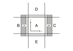
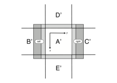
Figure 1: The interaction between sweeps and rotations is illustrated for a process A with its four neighbouring processes B-E. The distributed data stored and treated in process A carries a small permanent buffer area (light shading) around all of its interfaces. An additional volatile buffer (dark shading) is added in the current $x$-direction. The $x$-sweep is performed horizontally. For the $y$-sweep, the data and the permanent buffer are rotated clockwise by $90$ degrees such that the $y$-sweep can also be performed in the horizontal direction.

Figure 1 shows the computational domain of a process A after the cuboidal domain decomposition. The data stored and updated in process A is surrounded by a small permanent buffer zone (light shading). In the current $x$-direction, there is an additional volatile buffer zone (dark shading). At the beginning of a time step, the overlapping data from process B is communicated to process A in order to update the buffer designated by ’left’. The overlapping data communicated from process C fills the buffer designated by ’right’. During the communication, the horizontal sweep in $x$-direction can already start to work on the interior zones that don’t require the communicated buffer zones. Once all data has arrived, the $x$-sweep can be completed so that all zones in domain A and the permanent buffer is up to date. Hence communication is overlapped with computation.

For the sweep in $y$-direction, all local data in Figure 1 are rotated clockwise by $90$ degrees so that the $y$-direction becomes horizontal. This time it is the data of process E that need to be communicated to the buffer zones designated by ’left’ and the data of process D that need to be communicated to the buffer zones designated by ’right’. Again, the sweep can start with the inner zones and update the border zones once the communications have completed. The important point is to realise that the $y$-sweep is now also applied in the horizontal direction so that the one-dimensional subroutines used for the $x$-sweep can be used without any modifications. In the three-dimensional code, the procedure is repeated a third time for the sweeps in $z$-direction. Finally, all three sweeps are once more applied in reverse order to obtain second order accuracy. This ordering of the sweeps requires four rotations between the six directional sweeps.

Hence, the communication pattern is the only action that needs to be performed differently during the different sweeps: For the $x$-sweep we need to copy $B\longrightarrow A\left(\textrm{left}\right)$ and $C\longrightarrow A\left(\textrm{right }\right)$, while for the $y$-sweep we need to copy $E\longrightarrow A\left(\textrm{left}\right)$ and $D\longrightarrow A\left(\textrm{right}\right)$. This distinction can easily be implemented using persistent communications in the MPI. When the code is initialised, the communications $B\longrightarrow A\left(\textrm{left}\right)$ and $C\longrightarrow A\left(\textrm{right }\right)$are defined to be invoked by a handle $h_{x}$, while the communications $E\longrightarrow A\left(\textrm{left}\right)$ and $D\longrightarrow A\left(\textrm{right}\right)$are defined to be invoked by a handle $h_{y}$. With this preparation it is straightforward to perform the $x$-sweep by calling a function $\mathtt{sweep}\left(h_{x},n_{x},n_{y},A,\mathtt{f}\right)$ and the $y$-sweep by calling the same function $\mathtt{sweep}\left(h_{y},n_{y},n_{x},A^{\prime},\mathtt{f}\right)$, where $n_{x}$ and $n_{y}$ specify the dimensions of $A$, where $A^{\prime}$ is the rotated state of $A$ and where $\mathtt{f}$ points to a one-dimensional function that implements the physical equations treated by the sweep. In this way, the setup of the communication topology during the initialisation of the code, the trigger of communications and the dimensional index gymnastics in the $\mathtt{sweep}$ subroutine, and the implementation of the physics in the function $\mathtt{f}$ are all very well disentangled.

The repeated evaluation of the physics equations in the function $\mathtt{f}$ amounts to the dominant contribution to the total CPU-time. Because the sweeps are now always performed along contiguous memory, it is possible to pipeline the physics quantities in the cache so that the access of the large data arrays is reduced to a minimum. The first order predictor and second order corrector are evaluated according to the following scheme:

loop over cells i in x-direction
  u3 = u4
  u4 = u5
  u5 = u6
  u6 = u(i)
  if i<3 cycle
  uu1 = uu2
  uu2 = uu3
  uu3 = uu4
  uu4 = uu5
  uu5 = u5 + rate(u4,u5,u6)*0.5*dt !first order
  if i<7 cycle
  u(i-3) = u3 + rate(uu1,uu2,uu3,uu4,uu5)*dt !second order
end loop over cells

Here, $u(i)$ is the state vector with the conserved variables, which is only involved twice per time step $dt$, once for data retrieval and once for data storage. The hydrodynamics equations of Eq. (36) and their discretisation described in Eqs. (41) and (43) are abbreviated here by the evaluation of $\mathtt{rate()}$. The whole operation has a stencil of $7$ cells and will lead to $3$ unassigned cells at each end of the array $u$. Hence, the buffer in Fig. 1 has to be large enough to host the unassigned cells.

Note that the horizontal sweep in $x$-direction is performed independently for all $n_{y}$ rows of the data in process $A$. Hence it is straightforward to further parallelise the loop over the rows $i_{y}=1\ldots n_{l}$ with OpenMP, where $n_{l}=n_{y}+2n_{bp}$ is the dimension of $A$ including the permanent buffer of width $n_{bp}$ on either side. This one OpenMP parallel section suffices to parallelise over 90% of the workload of the code for shared memory nodes. Hence, the above-described approach naturally leads to a hybrid parallelisation, where MPI is used to distribute the memory by the cuboidal domain decomposition across different nodes or processors, while OpenMP is used to parallelise the loop over the rows along the current sweep direction on the cores that are available to each node or processor.

We evaluated the strong scaling of fish on the new ROSA system (Cray XT-5, nodes with 2 quad-core AMD Opteron 2.4 GHz Shanghai processors, SeaStar 2.2 communications processor with 2 GBytes/s of injection bandwidth per node) at the Swiss National Supercomputer Center (CSCS). The dominant limitation to the scaling of fish is the rather large stencil that emerges from the combination of the MHD and hydrodynamics solver with a first and second order step in a single sweep. fish scales without problem if the problem size is increased with the increased number of processors. More interesting is the case of a fixed size problem. Figure 2 shows the strong scaling for a problem with $600^{3}$ cells. As the number of processors is increased, the ratio of buffer zones to volume zones increases as well. In this case it is the evaluation of the physics equations on the buffer zones that limit the efficiency. However, Fig. 2 also shows that fish scales very nicely to of order $10000$ processors in the hybrid MPI/OpenMP mode where MPI is used between nodes and OpenMP within the node. This scaling can be achieved because the parallelisation with OpenMP does not increase the number of buffer zones. A version of fish with smaller stencils is under development.

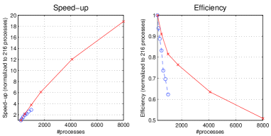
Figure 2: Strong scaling of the fish code. The speedup, normalised to 216 processes, is shown on the left hand side. The efficiency is displayed on the right hand side. The dashed lines with data points taken at the circles refer to a parallelisation that uses only MPI. The solid lines with data points taken at the crosses refer to a hybrid parallelisation with MPI between nodes and OpenMP within nodes. The problem size was kept constant at $600^{3}$ cells. The deviation from perfect scaling is rather due to the increase of work on buffer zones with respect to the work on volume zones than a bottleneck in the communication.

4 Numerical results

In this section we verify our code by performing several multidimensional test simulations of astrophysical interest. The algorithm has already been tested for second order accuracy in [13] and we do not repeat that here. Unless otherwise stated, we use periodic boundary conditions for all test problems. The simulations are stopped before any interaction due to the periodic boundary can occur.

4.1 Circularly polarised Alfvén waves

Our first test problem involves the propagation of circularly polarised Alfén waves. These waves are a smooth exact non-linear solution to the equations of ideal MHD [24] and represent therefore an ideal problem to test the convergence of numerical methods.

We have used the same initial conditions [36]. Circularly polarised Alfvén waves are propagated the $x-y$ plane at an angle of $\alpha=30^{\circ}$ with respect to the $x$-axis. The domain is set to $[0,1/\cos\alpha]\times[0,1/\sin\alpha]$ and discretised with $N\times N$ cells where $N=32,64,128,256,512$. The adiabatic index is set to $\gamma=5/3$. Then we have $\rho=1$, $v_{\parallel}=0$, $p=0.1$, $b_{\parallel}=1$, $v_{\perp}=b_{\perp}=A\sin[2\pi(x\cos\alpha+y\sin\alpha)]$ and $v_{z}=b_{z}=A\cos[2\pi(x\cos\alpha+y\sin\alpha)]$. The subscript $\parallel$ and $\perp$ denote the components parallel and perpendicular to the wave propagation, respectively. We have set the wave amplitude to $A=0.1$. With these parameters the Alfvén velocity is $B_{\parallel}\rho=1$ and therefore the wave profile is advected to its initial position after a simulation time $t=1$.

In figure 3 are shown the numerical errors after the wave profile crossed the domain once $t=1$. The error is given by the L1 norm of the difference between the initial conditions and the numerical solution at time $t=1$ over all cells:

$$\delta\boldsymbol{u}=\frac{1}{N^{2}}\sum_{i,j}\mid\boldsymbol{u}_{i,j}^{n}-\boldsymbol{u}_{i,j}^{0}\mid.$$

To get the absolute numerical error we have summed over all components of $\delta\boldsymbol{u}$. The scheme shows second order accuracy as can be inferred from figure 3.

Figure 3: Convergence for circularly polarised Alfvén waves. The points are the absolute numerical error as function of the number of grid points. The solid line is a reference second order rate.

4.2 Sedov-Taylor blast wave

The Sedov-Taylor blastwave test is a purely hydrodynamical test involving a strong spherically symmetric outward propagating shock wave. An analytical self-similar solution can be found for example in [39, 40]. We use an adiabatic index of $\gamma=5/3$. The problem is solved on a cubic domain $(x,y,z)\in[0,1]^{3}$ with $256^{3}$ computational cells and equidistant mesh spacing.

The density is set to unity and the velocity to zero throughout the whole domain. A huge amount of internal energy $e=3\times 10^{3}$ is placed uniformly in a small spherical region of radius $0.01$ at the center of the domain. Outside the spherical region the energy is set to $e=1\times 10^{-3}$. The energy amount concentrated at the center then starts a strong shock wave which propagates spherically outward from the center of the domain. The simulation was stopped at time $t=1.7419\times 10^{-4}$ when the shock has propagated to a distance $r\approx 0.45$ from the center. In figure 4 a random subset of cells (blue points) and a radial average of the numerical solution (green) are compared against the exact solution (red). All the values have been normalized to the exact postshock value. The postshock values of the numerical solution are lower but come close to the exact solution. Despite we have a dimensionally split code, the scattering of the points at the shock is not dramatic when compared to the Cartesian grid size of $\Delta x=\Delta y=\Delta z\approx 0.004$. In figure 5 a shaded surface plot is shown for the density in the $x,y$ plane with $z=1/2$. As seen in the figure, the shock looks spherical and no serious symmetry breaking due to the dimensionally split character of the code can be seen.

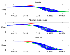
Figure 4: Radial distribution of the Sedov-Taylor blast wave test. The blue points represent a random subset of all the cells, the green line is a radial average of the numerical solution and the red line is the exact solution. All values have been normalized to the exact postshock values. The ticks on the $r$ axis have the size of the mesh spacing $\Delta x$ and the shock is resolved within roughly $2\Delta x$.

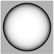
Figure 5: Shaded surface plot of the density for the Sedov-Taylor blast wave in the $x,y$ plane with $z=1/2$ illustrating the spherical symmetric character of the numerical solution.

4.3 Spherical Riemann problem

This problem is a spherical setup of Sod’s shocktube and was suggested in [28] as a test for multidimensional hydrodynamics codes. The solution is computed on a cubic domain $(x,y,z)\in[0,1]^{3}$ with $256^{3}$ computational cells and equidistant mesh spacing. Once again, an adiabatic index $\gamma=5/3$ is used.

The domain is decomposed into a spherical region of radius $R=0.25$ at the center of the domain and the remaining exterior region. The fluid variables are set to constant values in each region. At the boundary between both regions a circular discontinuity results. In both regions, the velocity is set to zero. In the inner region we set the density $\rho=0.125$ and the pressure $p=0.1$. In the outer region, we set the density $\rho=1$ and the pressure $p=1$. The simulation is stopped at time $t=0.09$.

In figure 6 the density distribution at the end of the simulation is displayed. The blue points are a random subset of cells, the green line is a radial average of the numerical solution and the red line is a highly resolved numerical solution from a 1D spherically symmetric code based on the same algorithm as the 3D one. The shock, the contact discontinuity and the rarefaction wave are well captured by the 3D code. The scattering of the points is strongest at the inward propagating shock. In figure 7 a shaded surface plot of the density in the $x,y$ plane with $z=1/2$ is pictured. The spherical character of the solution is well retained and the dimensional splitting does not degrade this symmetry.

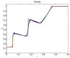
Figure 6: Radial density distribution of the spherical Riemann problem. The blue points represent a random subset of all the cells, the green line is an average over all the cells and the red line is the result of a highly resolved 1D simulation.

Figure 7: Shaded surface plot of the density for the spherical Riemann problem in the $x,y$ plane with $z=1/2$ illustrating the spherically symmetric character of the numerical solution. The density ranges from 1 (black) to 0.125 (white).

4.4 Magnetic explosion

This test is based on the same idea as the Sedov-Taylor blastwave problem with the addition of a magnetic field We used the same domain, number of cells and adiabatic index. The density is set to $\rho=1$ and the velocity to vanish everywhere in the domain. At the center of the domain we set the pressure $P=100$ in a spherical region with radius $R=0.1$. Outside of a sphere with radius $R=0.125$ we set the pressure to $P=1$. In the spherical shell between the high central pressure and the outer low pressure regions, we let the pressure vary linearly between the two extremes. The magnetic field components are set as $b_{x}=b_{y}=7/\sqrt{(}2)$ and $b_{z}=0$. Inside the high pressure sphere the ratio between gas pressure and magnetic pressure is $\beta=2P/B^{2}\approx 4$ and outside it is $\beta=2P/B^{2}\approx 0.04$. This is a difficult test problem for codes evolving the total energy: The internal energy is obtained by the substraction of kinetic and magnetic energy from the total energy. When the energy density is locally dominated by the magnetic field, negative internal energies can occur which then break down the simulation.

The simulation was stopped at $t=0.03$ and we used a CFL number of $0.5$. For the fluid update we used the minmod limiter. The results are displayed in figure 8 for the density, pressure, kinetic energy and magnetic energy. As apparent from the figure, spherical symmetry is broken and one clearly distinguishes between the flow propagation parallel and orthogonal to the magnetic field. The outermost shell indicates a fast magnetosonic shock, which is only weakly compressive. The energy density is dominated by the magnetic field. On the inside there are two dense shells propagating parallel to the magnetic field. From the outside these dense shells are bound by a slow magnetosonic shock and a contact on the inside.

Similar initial conditions can be found in the literature, see e.g. [41, 42, 43]. We have tried to run our code with the same initial conditions as in ref. [44] where the magnetic field is higher $b_{x}=b_{y}=10/\sqrt{(}2)$ and with no linear interpolation between the high and low pressure regions. However, we didn’t succeed under reasonable CFL conditions ($>0.05$) and simulation time. The appearance of negative internal energies always stopped the simulation. For very low $\beta$ flows we pay the price for the algorithmic simplicity of splitting fluid and magnetic advection. An upwind interpolation of the velocities to cell faces might help to cure the problem. However, we have not yet explored this possibility.

Figure 8: Shaded surface plot of the magnetic explosion at time $t=0.03$. Density (top left) ranges from 0.24 (white) to 2.17 (black). Gas pressure (top right) ranges from 0.25 (white) to 15.85 (black). Magnetic energy (bottom left) ranges from 7.66 (white) to 33.50 (black). Kinetic energy (bottom right) ranges from 0 (white) to 17.33 (black).

4.5 The rotor problem

Our next test is the so-called rotor problem, presented in [41]. We use the first rotor problem in [36] as initial conditions. We solve this 2D problem in the Cartesian domain $[0,1]^{2}$ with $256^{2}$ computational cells. The problem consists of a dense rapidly rotating cylinder (the rotor) with $\rho=10$, $v_{x}=-2(y-1/2)/r_{0}$, $v_{y}=2(x-1/2)/r_{0}$ extending up to a radius $r_{0}=0.1$, where $r=[(x-1/2)^{2}+(y-1/2)^{2}]^{1/2}$, installed in a lighter resting fluid. The lighter fluid is characterized by $\rho=1$, $v_{x}=v_{y}=0$ for $r>r_{1}=0.115$. In between the rotating and the light fluid $r_{0}<r<r_{1}$ we set

$$\rho = 1+9f(r)$$

$$v_{x} = -2f(r)(y-1/2)/r$$

$$v_{y} = 2f(r)(x-1/2)/r$$

where

$$f(r)=\frac{r_{1}-r}{r_{1}-r_{0}}.$$

This smoothes out the discontinuities and reduces initial transients. The magnetic field is initially set to $b_{x}=5/\sqrt{4\pi}$, $b_{y}=b_{z}=0$ and the pressure is uniformly set to $p=1$. The adiabatic index used for this test is $\gamma=1.4$.

The simulation was run to time $t=0.15$ and the results are displayed in figure 9. The dense rotating cylinder initially not in equilibrium has started to expand until the magnetic pressure due to field wrapping has stopped the expansion resulting in its oblate shape. The outer layers of the dense cylinder has lost part of its initial angular momentum in form of Alvén waves radiating away. This braking of the magnetic rotor is a possible model for the angular momentum loss of collapsing gas clouds in star formation [45, 46].

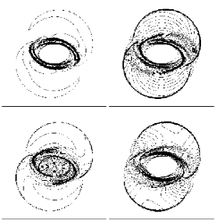
Figure 9: Contour plot of the rotor problem at time $t=0.15$. The density (top left), the gas pressure (top right), the Mach number (bottom left) and the magnetic pressure (bottom right).

4.6 Two dimensional MHD Riemann problem

The next test we performed is a two dimensional Riemann problem. The initial conditions are similar to [47]:

$$\left(\rho,v_{x},v_{y},v_{z},P\right)=\left\{\begin{array}[]{r r r r}\left(\right.1,&-0.75,&0.5,&0.,1.\left.\right),\;x\leq L_{x}/2,\;y\leq L_{y}/2\\ \left(\right.3,&-0.75,&-0.5,&0.,1.\left.\right),\;x>L_{x}/2,\;y\leq L_{y}/2\\ \left(\right.2,&0.75,&0.5,&0.,1.\left.\right),\;x\leq L_{x}/2,\;y>L_{y}/2\\ \left(\right.1,&0.75,&-0.5,&0.,1.\left.\right),\;x>L_{x}/2,\;y>L_{y}/2\\ \end{array}\right.$$

and the magnetic field is uniformly $\boldsymbol{b}=\left(2,0,1\right)/\sqrt{4\pi}$. We setup the problem on the domain $[0,0.8]^{2}$ and hence $L_{x}=0.8$, $L_{y}=0.8$ with $512^{2}$ cells. The adiabatic index is set to $\gamma=5/3$. For this test we used zeroth order extrapolation boundary conditions and evolved the problem to time $t=0.8$ The density, pressure, kinetic energy and magnetic energy are displayed in figure 10. A similar test problem can also be found in [48]. Our results compare qualitatively well with the cited references.

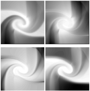
Figure 10: Contour plot of the 2D MHD Riemann problem at time $t=0.8$. Density (top left) ranges from 0.3428 (white) to 2.5698 (black). Gas pressure (top right) ranges from 0.1208 (white) to 0.7757 (black). Magnetic energy (bottom left) ranges from 0.0039 (white) to 0.2953 (black). Kinetic energy (bottom right) ranges from 0 (white) to 0.6233 (black).

4.7 Steady polytrope

As a final test, we show the performance of our HSE correction scheme on an astrophysical problem. We simulate a model star, a so-called polytrope [1]. These model stars are constructed in spherical symmetry from hydrostatic equilibrium

$$\frac{\mathrm{d}p}{\mathrm{d}r}=-\rho\frac{\mathrm{d}\phi}{\mathrm{d}r}$$ (71)

and Poisson’s equation

$$\frac{1}{r^{2}}\frac{\mathrm{d}}{\mathrm{d}r}\left(r^{2}\frac{\mathrm{d}\phi}{\mathrm{d}r}\right)=4\pi G\rho$$ (72)

where $r$ is the radial variable and $G$ is the gravitational constant. The functional relation between $p$ and $\rho$ is of the form $p=\kappa\rho^{\gamma}$ where $\kappa$ and $\gamma$ are constants. This relation is called a polytropic equation of state, $\kappa$ is the polytropic constant and $\gamma$ the polytropic exponent not to be confused here with the adiabatic index. We chose the following parameters: $M=1M_{\odot}$, $R=1R_{\odot}$ and $\gamma=4/3$. Here $M$ is the total mass of the star in units of solar masses and $R$ is the radius of the star in units of solar radii. With these parameters eq. (71) and (72) can easily be solved by any ODE integrator. The resulting star has then a polytropic constant $\kappa\approx 3.841\times 10^{14}$ (in cgs units) and a mean density of $\overline{\rho}\approx 1.408$ $\mathrm{g/cm}^{3}$. This sets the hydrostatic timescale $\tau_{\mathrm{HSE}}$ $\approx$ $(\overline{\rho}G)^{-1/2}/2$ $\approx$ $1.631\times 10^{3}\mathrm{s}$, which is the characteristic timescale on which the star reacts to perturbations of its hydrostatic equilibrium. We then mapped the spherical profiles of the density, internal energy and gravitational potential onto a 3D Cartesian grid of dimensions $[0,2.9R_{\odot}]^{3}$ such that the center of the star coincides with the center of the domain. We have put around the star a low density atmosphere $\rho_{\mathrm{atm}}=10^{-6}\rho_{C}$ where $\rho_{C}=76.313$ $\mathrm{g/cm}^{3}$ is the central density. The low density atmosphere is not in hydrostatic equilibrium but since its mass is so low it will have little dynamic effect on the star. We adopted continuous boundary conditions.

We then evolve the hydrodynamic variables for $20$ hydrostatic timescales $\tau_{\mathrm{HSE}}$ with the ideal gas law (5), $\gamma=4/3$, and with the unsplit source term integrator described in 2.3. The gravitational potential is kept fixed for the whole simulation. We have used both $64^{3}$ and $128^{3}$ cells to discretise the domain.

The results of the simulation are shown in figure 11. The subplot on the left hand side shows the spherically averaged density distribution of the simulation with $128^{3}$ cells resolution with and without the HSE correction (dash dotted and solid red lines respectively). The solid blue line is the density profile as initially put on the 3D grid and is therefore the reference solution. The subplot on the right hand side shows the central density normalised to the exact value as function of time in units of the hydrostatic timescale $\tau_{\mathrm{HSE}}$. The dash dotted lines are once again with the HSE correction while the solid lines are without. The blue lines have been computed with $64^{3}$ cells and the red lines with $128^{3}$ cells.

Due to the fact that the center of the star is an extremum in density and internal energy, any TVD scheme switches there to first order accuracy. Hence the strong numerical dissipation associated with first order accuracy heats the center of the star which increases the pressure and as a consequence the central density is diminished. In other words the star evaporates.

As can be seen from figure 11, the HSE correction effectively lowers this spurious effect. The HSE corrected simulation with $64^{3}$ cells (blue dash dotted on right subplot) does even better than the simulation with $128^{3}$ cells without correction.

With increasing resolution, as one expects, the effect of the HSE correction gets less dramatic. However, for low to intermediately resolved strong gravitationally induced gradients the HSE correction can greatly improve the accuracy at the center of the star.

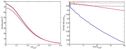
Figure 11: Left: radially averaged density for the simulation with $128^{3}$ cells with (dash dotted red line) and without (solid red line) HSE correction. The solid blue line is the reference solution. The HSE correction significantly increases the accuracy in the inner region. Right: central density normalised to the exact value as a function of time. The dash dotted and the solid lines again denote the simulation results with and without HSE correction. The blue lines were computed with $64^{3}$ cells and the red ones with $128^{3}$. The central density is kept nearly at constant value for the HSE corrected simulations while without the correction the central density decreases monotonically. Note the initial decrease in central density for all curves which is an initial relaxation of the numerical solution to the employed resolution.

5 Conclusion

We describe a simple and efficient three-dimensional implementation of the ideal magneto-hydrodynamics equations in our code named fish. The algorithms used are mostly based on [13]. Three different choices make the code very transparent and easy to work with: First, the rigorous operator splitting in second order operator ordering separates the sweeps across different coordinate directions. Also the constrained transport of the magnetic field is operator split from the hydrodynamics update. Second, the use of a Riemann solver free relaxation scheme with second order TVD advection facilitates the update of the state vector. Second order in time is achieved by a predictor-corrector approach within each time step. Third, subroutines for the physics operators are only required for the $x$-direction because the sweeps in $y$-direction and $z$-direction are performed by a rotation of the computational domain. Between the sweeps, the data is rotated such that an $x$-sweep in the direction of contiguous memory actually performs a $y$- or $z$-sweep in the coordinate frame of the rotated data. We document the details of an improved discretisation of the advective fluxes with respect to earlier versions of the code. Due to its clarity, we have successfully used the code for exercises and computational experiments in magneto-hydrodynamics classes.

We present different tests to evaluate the accuracy of fish. Second order convergence is demonstrated by the example of a circularly polarised propagating Alfven wave. The capability of accurately capturing hydrodynamic shocks is shown in a Sedov-Taylor blast wave explosion and in a spherical Riemann problem that are evolved in the three-dimensional computational domain. The latter two examples produce nice spherical flow features and show that the directional operator splitting does not cause sizeable asymmetries. We also investigate strong magnetosonic shocks in the form of a magnetic explosion. For this problem we reached a limit of the current scheme for very low plasma $\beta$ and very strong shocks. However, there is still room for improving the scheme in this extreme regimes and future developments will go in that direction. In order to further test the coupling between the magnetic fields and the fluid we perform the rotor problem in a two-dimensional computational domain. Finally, we calculate a 2D MHD Riemann problem and successfully compare the result with the literature. The only test that led to insufficient performance was the time evolution of a gravitationally bound hydrostatic object at low resolution. The problem is that the presence of gravitation leads to stationary density gradients that are mistaken as propagating wave gradients in the scheme that tailors the numerical dissipation for a total variation diminishing solution. The corresponding stationary dissipation leads to the evaporation of the bound object on few dynamical time scales. We remedied this problem by analytically estimating the hydrostatic gradients and subtracting them from the total gradients before calculating and applying the dissipation for the propagating waves. This to our knowledge novel and simple measure could also be used in combination with the Roe Riemann solver and potentially other approximate solvers. It allows the stable evolution of a gravitationally bound object over many dynamical time scales without exaggerated numerical dissipation at the center. This is shown in our last test case where we evolve a polytrope in hydrostatic equilibrium.

Inspite of the straightforward approach, fish is very efficient, even for problems containing $\sim 1000^{3}$ and more cells. fish implements cubic domain decomposition for distributed memory computer clusters. The process-wise rotation of the data between the sweeps takes about $10\%$ of the computational cost, but is largely compensated for by the fact that the individual sweeps along contiguous memory can be pipelined in the cache. The rotation of the data before the directional sweeps enables a very elegant parallelisation scheme that is based on non-blocking persistent MPI communication directives. We perform the communication for each direction separately and overlap it with computations of the update of interior cells. As sweeps along the same direction are embarassingly parallel within a shared memory cluster, we additionally parallelise those using OpenMP directives. With this, fish can take advantage of multi-core processors and scales nicely to $\sim 10000$ processes for a problem of fixed size. The limiting factor in the scaling of fish is the increasing ratio of work on buffer zones to work on enclosed zones. Even more processes can be used efficiently if the problem size grows with the number of available processes.

fish is mainly targeted for astrophysical applications where simple and efficient low-order algorithms are appreciated to accept manifold variations of input physics. The input physics is often a patchwork of different descriptions and algorithms for the different domains. As they do not always connect with a prescribed smoothness and as decisions about approximations are often taken during runtime, it is difficult to work with higher order methods. fish has successfully been used in one of the first predictions of the graviational wave signal from 3D supernova models with microscopic input physics [15] and provides the foundation for the implementation of spectral neutrino transport in our new code ELEPHANT (ELegant and Efficient Parallel Hydrodynamics with Approximate Neutrino Transport) [16]. The dynamical contrast of the density in many astrophysical applications suggests the implementation of an adaptive mesh. We discussed the extension of the approach to non-uniform orthogonal meshes, but find them only applicable for limited dynamical contrasts of about a factor of two increase of the resolution. On the long term, it appears more promising to embed the uniform Cartesian mesh of our current approach in a multi-patch driver like e.g. carpet in the cactus framework. We hope that this paper will serve as a reference for future users and developers of the public version of fish, which is in preparation and will soon become available.

References

- [1] S. Chandrasekhar, An introduction to the study of stellar structure (New York: Dover, 1967).
- [2] J. H. Lane, American Journal of Science 50, 57 (1869).
- [3] V. Springel, N. Yoshida, and S. D. M. White, New Astronomy 6, 79 (2001).
- [4] J. M. Blondin and E. A. Lufkin, ApJS88, 589 (1993).
- [5] J. M. Stone, D. Mihalas, and M. L. Norman, ApJS80, 819 (1992).
- [6] J. M. Stone and M. L. Norman, ApJ413, 198 (1993).
- [7] J. M. Stone and M. L. Norman, ApJ413, 210 (1993).
- [8] A. C. Calder et al., ApJS143, 201 (2002).
- [9] B. Fryxell et al., ApJS131, 273 (2000).
- [10] B. Giacomazzo and L. Rezzolla, Classical and Quantum Gravity 24, 235 (2007).
- [11] J. M. Stone et al., ApJS178, 137 (2008).
- [12] B. W. O’Shea et al., ArXiv Astrophysics e-prints (2004), arXiv:astro-ph/0403044.
- [13] U.-L. Pen, P. Arras, and S. Wong, ApJS149, 447 (2003).
- [14] U.-L. Pen, C. D. Matzner, and S. Wong, ApJ596, L207 (2003).
- [15] S. Scheidegger, T. Fischer, S. C. Whitehouse, and M. Liebendörfer, A&A490, 231 (2008), 0709.0168.
- [16] M. Liebendörfer, S. C. Whitehouse, and T. Fischer, ApJ698, 1174 (2009), 0711.2929.
- [17] A. A. Barmin, A. G. Kulikovskiy, and N. V. Pogorelov, J. Comput. Phys. 126, 77 (1996).
- [18] R. J. LeVeque, D. Mihalas, and E. A. Dorfi, Computational Methods for Astrophysical Fluid Flow (Springer, Berlin, 2005).
- [19] M. Torrilhon, J. Plasma Phys. 69, 253 (2003).
- [20] J. U. Brackbill and D. C. Barnes, J. Comput. Phys. 35, 426 (1980).
- [21] S. Jin and Z. Xin, Comm. Pure and Appl. Math. 48, 235 (1995).
- [22] C. R. Evans and J. F. Hawley, ApJ332, 659 (1988).
- [23] G. Strang, SIAM J. Num. Anal. 5, 506 (1968).
- [24] L. D. Landau and E. M. Lifschitz, Lehrbuch der theoretischen Physik, 10 Bde., Bd.8, Elektrodynamik der Kontinua (Deutsch (Harri), 1991).
- [25] R. Courant, K. Friedrichs, and H. Lewy, Mathematische Annalen 100, 32 (1928).
- [26] S. K. Godunov, Mat. Sb. (N.S.) 47 (89), 271 (1959).
- [27] C. B. Laney, Computational Gasdynamics (Cambridge University Press, 1998).
- [28] E. F. Toro, Riemann Solvers and Numerical Methods for Fluid Dynamics. A Practical Introduction (Springer-Verlag GmbH, 1997).
- [29] R. J. LeVeque and M. Pelanti, J. Comput. Phys. 172, 572 (2001).
- [30] R. J. LeVeque, Numerical Methods for Conservation Laws (Birkhäuser, 1992).
- [31] M. Zingale et al., ApJS143, 539 (2002).
- [32] J. U. Brackbill and D. C. Barnes, J. Comput. Phys. 35, 426 (1980).
- [33] P. Londrillo and L. Del Zanna, J. Comput. Phys. 195, 17 (2004).
- [34] J. A. Rossmanith, SIAM J. Sci. Comput. 28, 1766 (2006).
- [35] M. Torrilhon and M. Fey, SIAM J. Num. Anal. 42, 1694 (2004).
- [36] G. Tóth, J. Comput. Phys. 161, 605 (2000).
- [37] J. D. Jackson, Classical Electrodynamics Third Edition (Wiley, 1998).
- [38] M. Vinokur, J. Comput. Phys. 81, 1 (1989).
- [39] L. D. Landau, E. M. Lifschitz, and W. Weller, Lehrbuch der theoretischen Physik, 10 Bde., Bd.6, Hydrodynamik (Deutsch (Harri), 1991).
- [40] G. B. Whitham, Linear and Nonlinear Waves (Pure and Applied Mathematics) (Wiley-Interscience, 1974).
- [41] D. S. Balsara and D. S. Spicer, J. Comput. Phys. 149, 270 (1999).
- [42] P. Londrillo and L. Del Zanna, ApJ530, 508 (2000).
- [43] A. L. Zachary, A. Malagoli, and P. Colella, SIAM J. Sci. Comput. 15, 263 (1994).
- [44] T. A. Gardiner and J. M. Stone, J. Comput. Phys. 227, 4123 (2008).
- [45] T. C. Mouschovias and E. V. Paleologou, ApJ237, 877 (1980).
- [46] T. C. Mouschovias and E. V. Paleologou, Moon and Planets 22, 31 (1980).
- [47] W. Dai and P. R. Woodward, J. Comput. Phys. 142, 331 (1998).
- [48] S. Serna, J. Comput. Phys. 228, 4232 (2009).
- [49] U.-L. Pen, ApJS115, 19-34 (1998).