Ergodic solenoids and generalized currents

Abstract.

We introduce the concept of solenoid as an abstract laminated space. We do a thorough study of solenoids, leading to the notion of ergodic and uniquely ergodic solenoids. We define generalized currents associated with immersions of oriented solenoids endowed with a transversal measure into smooth manifolds, generalizing Ruelle-Sullivan currents.

1. Introduction

This is the first of a series of articles [4, 5, 6, 7] in which we aim to give a geometric realization of real homology classes in smooth manifolds, by using immersed laminations, which we call solenoids. In this paper we define these structures, we carry a thorough study, and we construct the homology class associated to an oriented measured immersed solenoid in a smooth manifold.

Let $M$ be a smooth compact connected and oriented manifold of dimension $n\geq 1$ without boundary. Any closed oriented submanifold $N\subset M$ of dimension $0\leq k\leq n$ determines a homology class in $H_{k}(M,{\mathbb{Z}})$. This homology class in $H_{k}(M,{\mathbb{R}})$, as dual of De Rham cohomology, is explicitly given by integration of the restriction to $N$ of differential $k$-forms on $M$. Also, any immersion $f:N\to M$ defines an integer homology class in a similar way by integration of pull-backs of $k$-forms. Unfortunately, because of topological reasons dating back to Thom [11], not all integer homology classes in $H_{k}(M,{\mathbb{Z}})$ can be realized in such a way. Geometrically, we can realize any class in $H_{k}(M,{\mathbb{Z}})$ by topological $k$-chains. The real homology $H_{k}(M,{\mathbb{R}})$ classes are only realized by formal combinations with real coefficients of $k$-cells. This is not fully satisfactory. In particular, for a variety of reasons (for example, in the aim of developing a geometric intersection theory for real homology classes), it is important to have an explicit realization, as geometric as possible, of real homology classes.

In 1975, Ruelle and Sullivan [10] defined, for arbitrary dimension $0\leq k\leq n$, geometric currents by using oriented $k$-laminations embedded in $M$ and endowed with a transversal measure. They applied their results to the stable and unstable laminations of Axiom A diffeomorphisms (i.e. those with hyperbolic non-wandering set with a dense set of periodic orbits). The point of view of Ruelle and Sullivan is also based on duality. The observation is that $k$-forms can be integrated on each leaf of the lamination and then all over the lamination using the transversal measure. This makes sense locally in each flow-box, and then it can be extended globally by using a partition of unity. The result only depends on the cohomology class of the $k$-form. It is natural to ask whether it is possible to realize every real homology class using a Ruelle-Sullivan current. A first result, with a precedent in [2], confirms that this is not the case: homology classes with non-zero self-intersection cannot be represented by Ruelle-Sullivan currents with no compact leaves (see Theorem 10.1).

More precisely, for each Ruelle-Sullivan lamination with a non-atomic transversal measure, we can construct a smooth $(n-k)$-form which provides the dual in de Rham cohomology (see section 9). Using it, we prove that the self-intersection of a Ruelle-Sullivan current (for a lamination) is zero, therefore it is not possible to represent a real homology class in $H_{k}(M,{\mathbb{R}})$ with non-zero self-intersection (see section 10). This obstruction only exists when $n-k$ is even. This may be the historical reason behind the lack of results on the representation of an arbitrary homology class by Ruelle-Sullivan currents. In section 7 we review and extend Ruelle-Sullivan theory.

Therefore, in order to represent every real homology class we must first enlarge the class of Ruelle-Sullivan currents. This is done by considering immersions of abstract oriented solenoids. We define a $k$-solenoid to be a Hausdorff compact space foliated by $k$-dimensional leaves with finite dimensional transversal structure (see the precise definition in section 2).

For these oriented solenoids we can consider $k$-forms that we can integrate provided that we are given a transversal measure invariant by the holonomy group. We define an immersion of a solenoid $S$ into $M$ to be a regular map $f:S\to M$ that is an immersion in each leaf. If the solenoid $S$ is endowed with a transversal measure $\mu$, then any smooth $k$-form in $M$ can be pulled back to $S$ by $f$ and integrated. The resulting numerical value only depends on the cohomology class of the $k$-form. Therefore we have defined a closed current that we denote by $(f,S_{\mu})$ and call a generalized current. This defines a homology class $[f,S_{\mu}]\in H_{k}(M,{\mathbb{R}})$. Using these generalized currents, the above mentioned obstruction disappears. Actually in [6], we shall prove that every real homology class in $H_{k}(M,{\mathbb{R}})$ can be realized by a generalized current $(f,S_{\mu})$ where $S_{\mu}$ is an oriented measured immersed solenoid. Moreover in [7], it is shown that the set of such generalized currents $(f,S_{\mu})$ realizing a given real homology class $a\in H_{k}(M,{\mathbb{R}})$ is dense in the space of closed currents representing $a$.

But the space of solenoids is large, and we would like to realize the real homology classes by a minimal class of solenoids enjoying good properties. We are first naturally led to topological minimality. As we prove in section 2, the spaces of $k$-solenoids is inductive and therefore there are always minimal $k$-solenoids. However, the transversal structure and the holonomy group of minimal solenoids can have a rich structure, studied in sections 3 and 4. In particular, such a solenoid may have many different transversal measures, each one yielding a different generalized current for the same immersion $f$. Therefore, of particular interest are uniquely ergodic solenoids, with only one ergodic transversal measure. We study them in section 5.

We also make a thorough study of Riemannian solenoids. We identify transversal measures with the class of measures that disintegrate as volume along leaves (daval measures), and also prove a canonical decomposition of measures into a daval measure and a singular part, corresponding to the classical Lebesgue decomposition on manifolds (see section 6).

Acknowledgements.  The authors are grateful to Alberto Candel, Etienne Ghys, Nessim Sibony, Dennis Sullivan and Jaume Amorós for their comments and interest on this work. In particular, Etienne Ghys early pointed out on the impossibility of realization in general of integer homology classes by embedded manifolds. We thank the referee for a extremely careful reading of the manuscript and many suggestions.

2. Minimal solenoids

We first define abstract solenoids, which are the main tool in this article. As usual, $C^{\omega}$ denotes the space of analytic functions. By $r\leq\omega$, we mean that $r$ is an integer, that $r=\infty$ or that $r=\omega$.

Definition 2.1.

Let $0\leq s,r\leq\omega$, $r\geq s$, and let $k,\ell\geq 0$ be two integers. A foliated manifold (of dimension $k+\ell$, with $k$-dimensional leaves, of regularity $C^{r,s}$) is a smooth manifold $W$ of dimension $k+\ell$ endowed with an atlas ${\mathcal{A}}=\{(U_{i},\varphi_{i})\}$, $\varphi_{i}:U_{i}\to{\mathbb{R}}^{k}\times{\mathbb{R}}^{\ell}$, whose transition maps

$$\varphi_{ij}=\varphi_{i}\circ\varphi_{j}^{-1}:\varphi_{j}(U_{i}\cap U_{j})\to\varphi_{i}(U_{i}\cap U_{j})\ \,,$$

are of the form $\varphi_{ij}(x,y)=(X_{ij}(x,y),Y_{ij}(y))$, where $Y_{ij}(y)$ is of class $C^{s}$ and $X_{ij}(x,y)$ is of class $C^{r,s}$.

A flow-box for $W$ is a pair $(U,\varphi)$ consisting of an open subset $U\subset W$ and a map $\varphi:U\to{\mathbb{R}}^{k}\times{\mathbb{R}}^{\ell}$ such that ${\mathcal{A}}\cup\{(U,\varphi)\}$ is still an atlas for $W$.

Clearly an open subset of a foliated manifold is also a foliated manifold.

Given two foliated manifolds $W_{1}$, $W_{2}$ of dimension $k+\ell$, with $k$-dimensional leaves, and of regularity $C^{r,s}$, a regular map $f:W_{1}\to W_{2}$ is a continuous map which is locally, in flow-boxes, of the form $f(x,y)=(X(x,y),Y(y))$, where $Y$ is of class $C^{s}$ and $X$ is of class $C^{r,s}$.

A diffeomorphism $\phi:W_{1}\to W_{2}$ is a homeomorphism such that $\phi$ and $\phi^{-1}$ are both regular maps.

Definition 2.2.

($k$-solenoid) Let $0\leq r\leq s\leq\omega$, and let $k,\ell\geq 0$ be two integers. A pre-solenoid of dimension $k$, of class $C^{r,s}$ and transversal dimension $\ell$ is a pair $(S,W)$ where $W$ is a foliated manifold and $S\subset W$ is a compact subspace which is a union of leaves.

Two pre-solenoids $(S,W_{1})$ and $(S,W_{2})$ are equivalent if there are open subsets $U_{1}\subset W_{1}$, $U_{2}\subset W_{2}$ with $S\subset U_{1}$ and $S\subset U_{2}$, and a diffeomorphism $f:U_{1}\to U_{2}$ such that $f$ is the identity on $S$.

A $k$-solenoid of class $C^{r,s}$ and transversal dimension $\ell$ (or just a $k$-solenoid, or a solenoid) is an equivalence class of pre-solenoids.

We usually denote a solenoid by $S$, without making explicit mention of $W$. We shall say that $W$ defines the solenoid structure of $S$.

Definition 2.3.

(Flow-box) Let $S$ be a solenoid. A flow-box for $S$ is a pair $(U,\varphi)$ formed by an open subset $U\subset S$ and a homeomorphism

$$\varphi:U\to D^{k}\times K(U)\,,$$

where $D^{k}$ is the $k$-dimensional open ball and $K(U)\subset{\mathbb{R}}^{\ell}$, such that there exists a foliated manifold $W$ defining the solenoid structure of $S$, $S\subset W$, and a flow-box $\hat{\varphi}:\hat{U}\to{\mathbb{R}}^{k}\times{\mathbb{R}}^{\ell}$ for $W$, with $U=\hat{U}\cap S$, $\hat{\varphi}(U)=D^{k}\times K(U)\subset{\mathbb{R}}^{k}\times{\mathbb{R}}^{\ell}$ and $\varphi=\hat{\varphi}_{|U}$.

The set $K(U)$ is the transversal space of the flow-box. The dimension $\ell$ is the transversal dimension.

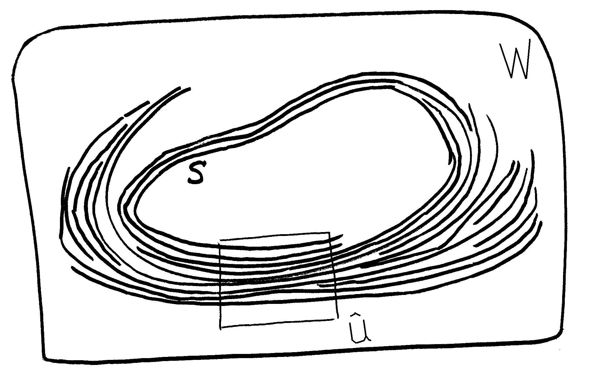
Figure 1. Flow-box

As $S$ is locally compact, any point of $S$ is contained in a flow-box $U$ whose closure $\overline{U}$ is contained in a bigger flow-box. For such flow-box, $\overline{U}\cong\overline{D}^{k}\times\overline{K}(U)$, where $\overline{D}^{k}$ is the closed unit ball, $\overline{K}(U)$ is some compact subspace of ${\mathbb{R}}^{\ell}$, and $U=D^{k}\times K(U)\subset\overline{D}^{k}\times\overline{K}(U)$. We might call these flow-boxes good. All flow-boxes that we shall use are of this type so we shall not append any appelative to them.

When the transversals of flow-boxes $K(U)\subset{\mathbb{R}}^{\ell}$ are open sets of ${\mathbb{R}}^{\ell}$ we talk about full transversals. In this case the solenoid structure is a $(k+\ell)$-dimensional compact manifold foliated by $k$-dimensional leaves.

Remark 2.4.

We refer to $k$ as the dimension of the solenoid and we write

$$k=\dim S\,.$$

Note that, contrary to manifolds, this dimension in general does not coincide with the topological dimension of $S$. The local structure and compactness imply that solenoids are metrizable topological spaces. The Hausdorff dimension of the transversals $K(U)$ is well defined and obviously bounded by the transversal dimension $\ell$. Thus, considering a finite covering by flow-boxes, we see that the Hausdorff dimension of $S$, $\dim_{H}S$, is well defined, and equal to

$$\dim_{H}S=k+\max_{U}\dim_{H}K(U)\leq k+\ell<+\infty\,.$$

Remark 2.5.

The definition of solenoid admits various generalizations. We could focus on intrinsic changes of charts in $S$ with some transverse Whitney regularity but without requiring a local diffeomorphism extension. Such a definition would be more general, but it is not necessary for our purposes. The present definition balances generality and simplicity.

Another alternative generalization would be to avoid any restrictive transversal assumption beyond continuity, and allow for transversals of flow-boxes any topological space $K(U)$. But a fruitful point of view is to regard the theory of solenoids as a generalization of the classical theory of manifolds. Therefore it is natural to restrict the definition only allowing finite dimensional transversal spaces. For an alternative approach see [3].

Definition 2.6.

(Diffeomorphisms of solenoids) Let $S_{1}$ and $S_{2}$ be two $k$-solenoids of class $C^{r,s}$ with the same transversal dimension. A $C^{r,s}$-diffeomorphism $f:S_{1}\to S_{2}$ is the restriction of a $C^{r,s}$-diffeomorphism $\hat{f}:W_{1}\to W_{2}$ of two foliated manifolds defining the solenoid structures of $S_{1}$ and $S_{2}$, respectively.

Remark 2.7.

A homeomorphism of solenoids is a diffeomorphism of class $C^{0,0}$.

This defines the category of smooth solenoids of a given regularity. Note that we have the subcategory of smooth solenoids with full transversals, and we have a forgetting functor into the category of smooth manifolds.

Definition 2.8.

(Leaf) A leaf of a $k$-solenoid $S$ is a leaf $l$ of any foliated manifold $W$ inducing the solenoid structure of $S$, such that $l\subset S$. Note that this notion is independent of $W$.

Note that $S\subset W$ is the union of a collection of leaves. Therefore, for a leaf $l$ of $W$ either $l\subset S$ or $l\cap S=\emptyset$.

Observe that when the transversals of flow-boxes $K(U)$ are totally disconnected then the leaf-equivalence coincides with path connection equivalence, and the leaves are the path connected components of $S$.

Definition 2.9.

(Oriented solenoid) An oriented solenoid is a solenoid $S$ such that there is a foliated manifold $W\supset S$ inducing the solenoid structure of $S$, where $W$ has oriented leaves.

It is easy to see that $S$ is oriented if and only if there is an orientation for the leaves of $S$ such that there is a covering by flow-boxes which preserve the orientation of the leaves.

Notice that we do not require $W$ to be oriented. For example, we can foliate a Möbius strip and create an oriented solenoid.

Definition 2.10.

We define ${\mathcal{S}}^{r,s}_{k,\ell}$ to be the space of $C^{r,s}$ $k$-solenoids with transversal dimension $\ell$.

Proposition 2.11.

Let $S_{0}\in{\mathcal{S}}_{k,\ell}^{r,s}$ be a solenoid. A non-empty compact subset $S$ of $S_{0}$ which is a union of leaves is a $k$-solenoid of class $C^{r,s}$ and transversal dimension $\ell$.

Proof.

Let $W$ be a $C^{r,s}$-foliated manifold defining the solenoid structure of $S_{0}$. Then $S\subset W$ and $W$ defines a $C^{r,s}$-solenoid structure for $S$.

Note that the flow-boxes of $S_{0}$ give, by restriction to $S$, flow-boxes for $S$. ∎

Corollary 2.12.

Connected components of solenoids ${\mathcal{S}}_{k,\ell}^{r,s}$ are in ${\mathcal{S}}_{k,\ell}^{r,s}$.

Theorem 2.13.

The space $({\mathcal{S}}_{k,\ell}^{r,s},\subset)$ ordered by inclusion is an inductive set.

Proof.

Let $(S_{n})\subset{\mathcal{S}}_{k,\ell}^{r,s}$ be a nested sequence of solenoids, $S_{n+1}\subset S_{n}$. Define

$$S_{\infty}=\bigcap_{n}S_{n}\,.$$

Then $S_{\infty}$ is a non-empty compact subset of $S_{1}$ as intersection of a nested sequence of such sets. It is also a union of leaves since each $S_{n}$ is so. Therefore by proposition 2.11, it is an element of ${\mathcal{S}}_{k,\ell}^{r,s}$. ∎

Corollary 2.14.

The space ${\mathcal{S}}_{k,\ell}^{r,s}$ has minimal elements.

Proposition 2.15.

If $S\in{\mathcal{S}}_{k,\ell}^{r,s}$ is minimal then $S$ is connected. $S$ is minimal if and only if all leafs of $S$ are dense.

Proof.

Each connected component of $S$ is a solenoid, thus by minimality $S$ must be connected.

Also the closure ${\overline{L}}$ of any leaf $L\subset S$ is a non-empty compact set union of leaves. Thus it is a solenoid and by minimality we must have ${\overline{L}}=S$.

Conversely, if $S$ is not minimal, then there is a proper sub-solenoid $S_{0}\subset S$. Take any leaf $l\subset S_{0}$. Then $l$ is not dense in $S$. ∎

3. Topological transversal structure of solenoids

Definition 3.1.

(Transversal) Let $S$ be a $k$-solenoid. A local transversal at a point $p\in S$ is a subset $T$ of $S$ with $p\in T$, such that there is a flow-box $(U,\varphi)$ of $S$ with $U$ a neighborhood of $p$ containing $T$ and such that

$$\varphi(T)=\{0\}\times K(U)\,.$$

A transversal $T$ of $S$ is a compact subset of $S$ such that for each $p\in T$ there is an open neighborhood $V$ of $p$ such that $V\cap T$ is a local transversal at $p$.

If $S$ is a $k$-solenoid of class $C^{r,s}$, then any transversal $T$ inherits an $\ell$-dimensional $C^{s}$-Whitney structure.

We clearly have:

Proposition 3.2.

The union of two disjoint transversals is a transversal.

Definition 3.3.

A transversal $T$ of $S$ is a global transversal if all leaves intersect $T$.

The next proposition is clear.

Proposition 3.4.

The union of two disjoint transversals, one of them global, is a global transversal.

Proposition 3.5.

If $S$ is minimal then all transversals are global. Moreover, if $S$ is minimal then any local transversal intersects all leaves of $S$.

Proof.

It is enough to see the second statement, since it implies the first. Let $U$ be a flow-box and $T=\varphi^{-1}(\{0\}\times K(U))$ a local transversal (see definition 2.3). By proposition 2.15, all leaves intersect $U$ and therefore they intersect $T$. ∎

Observe that the definition of solenoid with regular transverse structure says that $S$ is always embedded in a $(k+\ell)$-dimensional manifold $W$. Therefore $S\subset W$ has an interior and a boundary relative to $W$. These sets do not depend on the choice of $W$.

Definition 3.6.

(Proper interior and boundary) Let $S$ be a $k$-solenoid. Let $W$ be a foliated manifold defining the solenoid structure of $S$. The proper interior of $S$ is the interior of $S$ as a subset of $W$, considered as a $(k+\ell)$-dimensional manifold (where $\ell$ is the transversal dimension as usual).

The proper boundary of $S$ is defined as the complement in $S$ of the proper interior.

Let $\hat{\varphi}:\hat{U}\to{\mathbb{R}}^{k}\times{\mathbb{R}}^{\ell}$ be a flow-box for $W$ such that $U=\hat{U}\cap S$ and $\varphi=\hat{\varphi}_{|U}:U\to D^{k}\times K(U)$ is a flow-box for $S$. Then $K(U)\subset{\mathbb{R}}^{\ell}$. The proper interior, resp. the proper boundary, of $S$, intersected with $U$, consists of the collection of leaves $\varphi^{-1}(D^{k}\times\{y\})$, where $y\in K(U)$ is in the interior, resp. boundary, of $K(U)\subset{\mathbb{R}}^{\ell}$.

Note that the proper boundary of a solenoid that is a foliation of a manifold is empty. We have the converse, as follows from proposition 2.11.

Proposition 3.7.

If the proper boundary of $S$ is non-empty then it is a sub-solenoid of $S$.

Proposition 3.8.

Let $S\in{\mathcal{S}}$ be a minimal solenoid. If $S$ is not the foliation of a manifold then $S$ has empty proper interior, i.e. $K(U)\subset{\mathbb{R}}^{\ell}$ has empty interior for any flow-box $(U,\varphi)$.

Proof.

The proper boundary of $S$ is non-empty because otherwise, for each flow-box $U$, $K(U)\subset{\mathbb{R}}^{\ell}$ is an open set. Thus $S$ would be an open subset of $W$, where $W$ is a foliated manifold defining the solenoid structure of $S$, and so $S$ is itself a foliated $(k+l)$-manifold. This contradicts the assumption.

Now by minimality the proper boundary must coincide with $S$ and the proper interior is empty. ∎

Example 3.9.

The dyadic solenoid is obtained as follows. Let $T=\bar{D}^{2}\times S^{1}$ be the solid torus, and consider the standard embedding $\imath:T\to{\mathbb{R}}^{3}$. Let $f:T\to T$ be the embedding of $T$ into $T$ given by stretching the $\bar{D}^{2}$-direction and running over the $S^{1}$-direction twice (see Figure 2, such $f$ is a hyperbolic map). Let $T_{n}=\imath\circ f^{n}(T)$, $n\geq 0$, and consider $S=\bigcap_{n\geq 0}T_{n}$. Then $S$ is a $1$-solenoid with $2$-dimensional transversal structure. This can be seen as follows: consider a smooth foliation on $T_{0}-T_{1}$ which is standard near $\partial T_{0}=S^{1}\times S^{1}$ (i.e. with leaves $\{p\}\times S^{1}$), and which is equal to the foliation $f(\partial T_{0})$ on $\partial T_{1}$. We foliate $T_{n}-T_{n+1}$ by translating the foliation on $T_{0}-T_{1}$ via $f^{n}$. This gives a foliation on $T_{0}$, smooth on $T_{0}-S$, and of class $C^{\infty,0}$. So $S$ is a solenoid of class $C^{\infty,0}$.

It is easy to see that $S$ is homeomorphic to the topological space $\underleftarrow{\mathrm{lim}}\ \{g^{n}:S^{1}\to S^{1}\}$, where $g:S^{1}\to S^{1}$, $g(z)=z^{2}$. The above construction gives this space a solenoid structure.

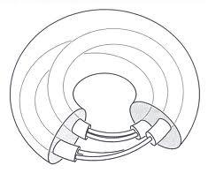
Figure 2. The dyadic solenoid

Solenoids with a one dimensional transversal will play a prominent role in [6]. We have for these the following structure theorem.

Theorem 3.10.

(Minimal solenoids with a $1$-dimensional transversal). Let $S\in{\mathcal{S}}$ be a minimal $k$-solenoid which admits a $1$-dimensional transversal $T$.

Then we have two cases:

1. $T$ is a finite union of circles, and $S$ is a $1$-dimensional foliation of a connected manifold of dimension $k+1$.

2. $T$ is totally disconnected, in which case we have two further possibilities:

   1. $T$ is a finite set and $S$ is a connected manifold of dimension $k$,

   2. $T$ is a Cantor set.

Proof.

We define the proper interior of $T$ as the intersection of the proper interior of $S$ with $T$. Now we have two cases.

If the proper interior of $T$ is non-empty, then the proper interior of $S$ is non-empty. Then the complement of the proper interior of $S$, if non-empty, is a sub-solenoid of $S$, contradicting minimality. Thus the proper interior of $S$ is all $S$, so the proper interior of $T$ is the whole of $T$. This means that any point $p\in T$ has a neighborhood (in $T$) homeomorphic to an interval. Therefore $T$ is a topological compact $1$-dimensional manifold, thus a finite union of circles. This ends the first case.

If the proper interior of $T$ is empty, then $T$ is totally disconnected. In this case, if $T$ has an isolated point $p$, then $S$ has only one leaf because by minimality any other leaf must accumulate the leaf containing $p$, and this is only possible if it coincides with it. Then $S$ is a $k$-dimensional connected manifold. If $T$ has no isolated points, then $T$ is non-empty, perfect, compact and totally disconnected, i.e. it is a Cantor set. ∎

4. Holonomy, Poincaré return and suspension

We study in this section the holonomy properties of solenoids, some of which are classical for foliations.

Definition 4.1.

(Holonomy) Given two points $p_{1}$ and $p_{2}$ in the same leaf, two local transversals $T_{1}$ and $T_{2}$, at $p_{1}$ and $p_{2}$ respectively, and a path $\gamma:[0,1]\to S$, contained in the leaf with endpoints $\gamma(0)=p_{1}$ and $\gamma(1)=p_{2}$, we define a germ of a map, the holonomy map,

$$h_{\gamma}:(T_{1},p_{1})\to(T_{2},p_{2})\,,$$

by lifting $\gamma$ to nearby leaves.

We denote by ${\operatorname{Hol}}_{S}(T_{1},T_{2})$ the set of germs of holonomy maps from $T_{1}$ to $T_{2}$.

Remark 4.2.

If $T_{1}$ and $T_{2}$ are global transversals then the sets of holonomy maps from $T_{1}$ to $T_{2}$ is non-empty. In particular, if $S$ is minimal the set of holonomy maps between two arbitrary local transversals is non-empty.

Definition 4.3.

(Holonomy pseudo-group) The holonomy pseudo-group of a local transversal $T$ is the pseudo-group of holonomy maps from $T$ into itself. We denote it by ${\operatorname{Hol}}_{S}(T)={\operatorname{Hol}}_{S}(T,T)$.

The holonomy pseudo-group of $S$ is the pseudo-group of all holonomy maps. We denote it by ${\operatorname{Hol}}_{S}$,

$${\operatorname{Hol}}_{S}=\bigcup_{T_{1},T_{2}}{\operatorname{Hol}}_{S}(T_{1},T_{2})\,.$$

Remark 4.4.

The orbit of a point $x\in S$ by the holonomy pseudo-group coincides with the leaf containing $x$.

Therefore, a solenoid $S$ is minimal if and only if the action of the holonomy pseudo-group is minimal, i.e. all orbits are dense.

The Poincaré return map construction reduces sometimes the holonomy to a classical dynamical system.

Definition 4.5.

(Poincaré return map) Let $S$ be an oriented minimal $1$-solenoid and $T$ be a local transversal. Then the holonomy return map is well defined for all points in $T$ and defines the Poincaré return map

$$R_{T}:T\to T\,.$$

The return map is well defined because in minimal solenoids “half” leaves are dense.

Lemma 4.6.

Let $S$ be a minimal $1$-solenoid. Let $p_{0}\in S$ and let $l_{0}\subset S$ be the leaf containing $p_{0}$. The point $p_{0}$ divides the leaf $l_{0}$ into two connected components. They are both dense in $S$.

Proof.

Consider one connected component of $l_{0}-\{p_{0}\}$, and let $C$ be its accumulation set. Then $C$ is non-empty, by compactness of $S$, and it is compact, as a closed subset of the compact solenoid $S$. It is also a union of leaves because if $l\subset S$ is a leaf, then $C\cap l$ is open in $l$ as is seen in flow-boxes, and also $C\cap l$ is closed in $l$. Therefore by connectedness of $l$, $C\cap l$ is empty or $l\subset C$.

We conclude that $C$ is a sub-solenoid, and by minimality we have $C=S$. ∎

When $S$ admits a global transversal (in particular when $S$ is minimal and admits a transversal) and the Poincaré return map is well defined, we have that it is continuous (without any assumption on minimality of $S$).

Proposition 4.7.

Let $S$ be an oriented $1$-solenoid and let $T$ be a global transversal such that the Poincaré return map $R_{T}$ is well defined. Then the holonomy return map $R_{T}$ is continuous. If the Poincaré return map for the reversed orientation of $S$ is also well defined, then $R_{T}$ is a homeomorphism of $T$. Moreover, if $S$ is a solenoid of class $C^{r,s}$ then $R_{T}$ is a $C^{s}$-diffeomorphism.

Proof.

The map $R_{T}$ is continuous because the inverse image of an open set is clearly open.

If the Poincaré return map $R_{T}^{-}$ for the same transversal obtained for the reverse orientation of $S$ is also well defined, then $R_{T}$ is bijective because by construction its inverse is $R_{T}^{-}$. Hence $R_{T}$ is a homeomorphism of $T$. Moreover, letting $W$ be a foliated manifold defining the solenoid structure of $S$, $T$ is a subset of an open manifold $U$ of dimension $l$, and the map $R_{T}$ extends as a homeomorphism $U_{1}\to U_{2}$, where $U_{1}$, $U_{2}$ are neighborhoods of $T$ (at least locally). If the transversal regularity of $S$ is $C^{s}$ then the local extension of $R_{T}$ is a $C^{s}$-diffeomorphism. ∎

When $T$ is only a local transversal then in general $R_{T}$ is not continuous. Nevertheless the discontinuities of $R_{T}$ are well controlled in practice and are innocuous when we deal with measure theoretic properties of $R_{T}$.

The suspension construction reverses Poincaré construction of the first return map.

Definition 4.8.

(Suspension construction) Let $X\subset{\mathbb{R}}^{\ell}$ be a compact set and let $f:X\to X$ be a homeomorphism which has a $C^{s}$-diffeomorphism extension to a neighborhood of $X$ in ${\mathbb{R}}^{\ell}$. The suspension of $f$ is the oriented $1$-solenoid $S_{f}$ defined by the suspension construction

$$S_{f}=([0,1]\times X)_{/(0,x)\sim(1,f(x))}\,.$$

Remark 4.9.

The solenoid $S_{f}$ has regularity $C^{\omega,s}$ (the transition maps are constructed with $f$).

The transversal $T=\{0\}\times X$ is a global transversal and the associated Poincaré return map $R_{T}:T\to T$ is well defined and equal to $f$.

In particular, the theory of dynamical systems for $X\subset{\mathbb{R}}^{\ell}$ and diffeomorphisms $f:X\to X$ (extending to a neighborhood of $X$) is contained in the theory of transversal structures of solenoids.

Note that example 3.9 is a $1$-solenoid constructed by suspension. The transversal $T$ is a Cantor set, homeomorphic to the $2$-adic integers ${\mathbb{Z}}_{2}$, and the suspension map is $f:{\mathbb{Z}}_{2}\to{\mathbb{Z}}_{2}$, $n\mapsto n+1$.

5. Measurable transversal structure of solenoids

In this section we study measure theory on solenoids, and in particular the measurable transverse structure.

Definition 5.1.

(Transversal measure) Let $S$ be a $k$-solenoid. A transversal measure $\mu=(\mu_{T})$ for $S$ is a collection of locally finite measures, each $\mu_{T}$ being associated to each local transversal $T$ and supported on $T$, which are invariant by the holonomy pseudo-group (see definition 4.3). More precisely, if $T_{1}$ and $T_{2}$ are two transversals and $h:V\subset T_{1}\to T_{2}$ is a holonomy map, then

$$h_{*}(\mu_{T_{1}}|_{V})=\mu_{T_{2}}|_{h(V)}\,.$$

We assume that a transversal measure $\mu$ is non-trivial, i.e. for some $T$, $\mu_{T}$ is non-zero.

We denote by $S_{\mu}$ a $k$-solenoid $S$ endowed with a transversal measure $\mu=(\mu_{T})$. We refer to $S_{\mu}$ as a measured solenoid.

Observe that for any transversal measure $\mu=(\mu_{T})$ the scalar multiple $c\,\mu=(c\,\mu_{T})$, where $c>0$, is also a transversal measure. Notice that there is no natural scalar normalization of transversal measures.

Definition 5.2.

(Support of a transversal measure) Let $\mu=(\mu_{T})$ be a transversal measure. We define the support of $\mu$ by

$$\operatorname{supp}\mu=\bigcup_{T}\operatorname{supp}\mu_{T}\,,$$

where the union runs over all local transversals $T$ of $S$.

Proposition 5.3.

The support of a transversal measure $\mu$ is a sub-solenoid of $S$.

Proof.

For any flow-box $U$, $\operatorname{supp}\mu\cap U$ is closed in $U$, since $\operatorname{supp}\mu_{K(U)}$ is closed in $K(U)$. Hence, $\operatorname{supp}\mu$ is closed in $S$. Also, locally in flow-boxes $\operatorname{supp}\mu$ contains full leaves of $U$. Therefore a leaf of $S$ is either disjoint from $\operatorname{supp}\mu$ or contained in $\operatorname{supp}\mu$. Also $\operatorname{supp}\mu$ is non-empty because $\mu$ is non-trivial. We conclude that $\operatorname{supp}\mu$ is a sub-solenoid. ∎

Definition 5.4.

(Transverse ergodicity) A transversal measure $\mu=(\mu_{T})$ on a solenoid $S$ is ergodic if for any Borel set $A\subset T$ invariant by the pseudo-group of holonomy maps on $T$, we have

$$\mu_{T}(A)=0\ \ {\hbox{\rm{ or }}}\ \ \mu_{T}(A)=\mu_{T}(T)\,.$$

We say that $S_{\mu}$ is an ergodic solenoid.

Definition 5.5.

(Transverse unique ergodicity) Let $S$ be a $k$-solenoid. The solenoid $S$ is transversally uniquely ergodic, or a uniquely ergodic solenoid, if $S$ has a unique up to scalars transversal measure $\mu$ and moreover $\operatorname{supp}\mu=S$.

Observe that in order to define these notions we only need continuous transversals. These ergodic notions are intrinsic and purely topological, i.e. if $S_{1}$ and $S_{2}$ are two homeomorphic solenoids by a homeomorphism $h:S_{1}\to S_{2}$, then $S_{1}$ is uniquely ergodic if and only if $S_{2}$ is. If $S_{1,\mu_{1}}$ and $S_{2,\mu_{2}}$ are homeomorphic and $\mu_{2}=h_{*}\mu_{1}$ via the homeomorphism $h:S_{1}\to S_{2}$, then $S_{1,\mu_{1}}$ is ergodic if and only if $S_{2,\mu_{2}}$ is.

These notions of ergodicity generalize the classical ones and do exactly correspond to the classical notions in the situation described by the next theorem.

Theorem 5.6.

Let $S$ be an oriented $1$-solenoid. Let $T$ be a global transversal such that the Poincaré return map $R_{T}:T\to T$ is well defined.

Then the solenoid $S$ is minimal, resp. ergodic, uniquely ergodic, if and only if $R_{T}$ is minimal, resp. ergodic, uniquely ergodic.

Proof.

We have by proposition 4.7 that $R_{T}$ is continuous. A leaf of $S$ is dense if and only if its intersection with $T$ is a dense orbit of $R_{T}$, hence the equivalence of minimality.

For the ergodicity, observe that we have a correspondence between measures on $T$ invariant by $R_{T}$ and transversal measures for $S$. Each transversal measure for $S$, locally defines a measure on $T$, hence defines a measure on $T$. Conversely, given a measure $\nu$ on $T$, we can transport $\nu$ in order to define a measure in each local transversal $T^{\prime}$ in the following way. We can define a map $R_{T^{\prime},T}:T^{\prime}\to T$ of first impact on $T$ by following leaves of $S$ from $T^{\prime}$ in the positive orientation. By the global character of the transversal this map is well defined. By construction $R_{T^{\prime},T}$ is injective. So we can define $\mu_{T^{\prime}}=R_{T^{\prime},T}^{*}\nu_{R_{T^{\prime},T}(T^{\prime})}$. Then $(\mu_{T^{\prime}})$ defines a transversal measure. The equivalence of unique ergodicity follows. Also $\nu$ is ergodic if and only $(\mu_{T^{\prime}})$ is ergodic because any decomposition of $\nu=\nu_{1}+\nu_{2}$ induces a decomposition of $(\mu_{T^{\prime}})$ by the transversal measures corresponding to the decomposing measures. ∎

When we have an ergodic oriented $1$-solenoid $S_{\mu}$ and $T$ is a local transversal, then the Poincaré return map is well defined $\mu_{T}$-almost everywhere and $\mu_{T}$ is ergodic.

Proposition 5.7.

Let $S$ be an oriented $1$-solenoid and let $T$ be a local transversal of $S$. Let $\mu$ be an ergodic transversal measure for $S$. Then the Poincaré return map $R_{T}$ is well defined for $\mu_{T}$-almost all points of $T$ and $\mu_{T}$ is an ergodic measure of $R_{T}$.

Proof.

Let $A_{T}\subset T$ be the set of wandering points of $T$, i.e. those points whose positive half leaves through them never meet $T$ again. Clearly $A_{T}$ is a Borel set. If $\mu_{T}(A_{T})\not=0$ we can decompose $\mu_{T}$ by decomposing $\mu_{T|A_{T}}$ and transporting the decomposition (back and forward) by the holonomy in order to decompose the transversal measure. Therefore $\mu_{T}(A_{T})=0$. As before, a decomposition of $\mu_{T}$ into invariant measures by $R_{T}$ yields a decomposition of the transversal measure $\mu$ invariant by holonomy. ∎

Recall that a dynamical system is minimal when all orbits are dense, and that uniquely ergodic dynamical systems are minimal. We have the same result for uniquely ergodic solenoids.

Proposition 5.8.

An oriented uniquely ergodic $1$-solenoid $S$ is minimal.

Proof.

If $S$ has a non-dense leaf $l\subset S$, we can consider a local transversal $T_{0}$ such that $T_{0}\cap\bar{l}\not=\emptyset$. Let $(l_{n})$ be an exhaustion of $l$ by compact subsets. Let $\mu_{n}$ be the atomic probability measure on $T_{0}$ equidistributed on the intersection of $l_{n}$ with $T_{0}$. Any limit measure $\mu_{n_{k}}\to\nu$ is a probability measure on $T_{0}$ with $\operatorname{supp}\nu\subset T_{0}\cap\bar{l}$. It follows easily that $\nu$ is invariant by the holonomy on $T_{0}$. Transporting by the holonomy, $\nu$ defines a transversal measure $\mu=(\mu_{T})$ (up to normalization, in each transversal it is also a limit of counting measures). But this contradicts unique ergodicity since $\operatorname{supp}\mu\not=S$. ∎

Given a measured solenoid $S_{\mu}$ we can talk about “$\mu$-almost all leaves” with respect to the transversal measure. More precisely, a Borel set of leaves has zero $\mu$-measure if the intersection of this set with any local transversal $T$ is a set of $\mu_{T}$-measure zero.

Now Poincaré recurrence theorem for classical dynamical systems translates as:

Proposition 5.9.

(Poincaré recurrence) Let $S_{\mu}$ be an ergodic oriented $1$-solenoid with $\operatorname{supp}\mu=S$. Then $\mu$-almost all leaves are dense and accumulate themselves.

Proof.

For each local transversal $T$ we know by proposition 5.7 that the Poincaré return map $R_{T}$ is defined for $\mu_{T}$-almost every point and leaves invariant $\mu_{T}$. Therefore by Poincaré recurrence theorem, $\mu_{T}$-almost every point has a dense orbit by $R_{T}$ in $\operatorname{supp}\mu_{T}=T$.

Observe that $S_{\mu}$ ergodic implies that $S$ is connected (otherwise we may decompose the invariant measure by restricting it to each connected component).

By compactness we can choose a finite number of local transversals $T_{i}=\varphi^{-1}(\{0\}\times K(U_{i}))$ with flow-boxes $\{U_{i}\}$ covering $S$. We can assume that we have that $U_{i}\cap U_{j}$ is a flow-box if non-empty. This assumption and the connectedness of $S$ imply that any Borel set of leaves that has either total or zero measure in a flow-box $U_{i}$, has the same property in $S$.

Now, the set of leaves $S_{i}$ that are non-dense in a given flow-box $U_{i}$ is of zero $\mu$-measure in $U_{i}$ (by Poincaré recurrence theorem applied to $R_{T_{i}}$). By the above, $S_{i}$ is of zero $\mu$-measure in $S$. Finally the set of non-dense leaves in $S$ is the finite union of the $S_{i}$, therefore is a set of leaves of zero $\mu$-measure. ∎

We denote by ${\mathcal{M}}_{\mathcal{T}}(S)$ the space of transversal positive measures on the solenoid $S$ equipped with the topology generated by weak convergence in each local transversal.

We denote by $\overline{\mathcal{M}}_{\mathcal{T}}(S)$ the quotient of ${\mathcal{M}}_{\mathcal{T}}(S)$ by positive scalar multiplication.

Proposition 5.10.

The space ${\mathcal{M}}_{\mathcal{T}}(S)$ is a cone in the vector space of all transversal signed measures ${\mathcal{V}}_{\mathcal{T}}(S)$. Extremal measures of ${\mathcal{M}}_{\mathcal{T}}(S)$ correspond to ergodic tranversal measures.

Proof.

Only the last part needs a proof. If $(\mu_{T})$ is not ergodic, then there exists a local tranversal $T_{0}$ and two disjoint Borel set $A,B\subset T_{0}$ invariant by holonomy with $\mu_{T_{0}}(A)\not=0$, $\mu_{T_{0}}(B)\not=0$ and $\mu_{T_{0}}(A)+\mu_{T_{0}}(B)=\mu_{T_{0}}({T_{0}})$. Let $S_{A}\subset S$, resp. $S_{B}\subset S$, be the union of leaves of the solenoid intersecting $A$, resp. $B$. These are Borel subsets of $S$. Let $(\mu_{T|T\cap S_{A}})$ and $(\mu_{T|T\cap S_{B}})$ be the transversal measures conditional to $T\cap S_{A}$, resp. $T\cap S_{B}$. Then

$$(\mu_{T})=(\mu_{T|T\cap S_{A}})+(\mu_{T|T\cap S_{B}})\,,$$

and $(\mu_{T})$ is not extremal. ∎

Corollary 5.11.

If ${\mathcal{M}}_{\mathcal{T}}(S)$ is non-empty then ${\mathcal{M}}_{\mathcal{T}}(S)$ contains ergodic measures.

We shall provide the proof of this result after theorem 6.8.

6. Riemannian solenoids

In this section we endow solenoids with a Riemannian structure and we study their metric properties.

All measures considered are Borel measures and all limits of measures are understood in the weak-* sense. We denote by ${\mathcal{M}}(S)$ the space of probability measures supported on $S$.

Definition 6.1.

(Riemannian solenoid) Let $S$ be a $k$-solenoid of class $C^{r,s}$ with $r\geq 1$. A Riemannian structure on $S$ is a Riemannian metric on the leaves of $S$ such that there is a foliated manifold $W$ defining the solenoid structure of $S$ and a metric $g_{W}$ on the leaves of $W$ of class $C^{r-1,s}$ such that $g=g_{W|S}$.

For instance, example 3.9 can be given a Riemannian structure by restricting the Riemannian metric of ${\mathbb{R}}^{3}$ to the leaves of the solenoid.

As for compact manifolds, via a partition of unity, any solenoid can be endowed with a Riemannian structure.

In the rest of this section $S$ denotes a Riemannian solenoid. Note that a Riemannian structure defines a $k$-volume on the leaves of $S$. This is a function $\operatorname{Vol}_{k}$ which assigns to any subset $A\subset l$ on a leaf $l\subset S$ its volume with respect to the Riemannian metric on the leaf.

Definition 6.2.

(Flow group) We define the flow group $G_{S}^{0}$ of a Riemannian $k$-solenoid $S$ as the group of $k$-volume preserving diffeomorphisms of $S$ isotopic to the identity in the group of diffeomorphims of $S$. We define the extended flow group $G_{S}$ as the group of $k$-volume preserving diffeomorphisms of $S$.

Note that we do not claim that $G_{S}^{0}$ is the connected component of the identity of $G_{S}$, although this may well be true.

Definition 6.3.

(daval measures) Let $\mu$ be a measure supported on $S$. The measure $\mu$ is a daval measure if it disintegrates as volume along leaves of $S$, i.e. for any flow-box $(U,\varphi)$ with local transversal $T=\varphi^{-1}(\{0\}\times K(U))$, we have a measure $\mu_{U,T}$ supported on $T$ such that for any Borel set $A\subset U$

$$\mu(A)=\int_{T}{\operatorname{Vol}}_{k}(A_{y})\ d\mu_{U,T}(y)\,,$$

where $A_{y}=A\cap\varphi^{-1}(D^{k}\times\{y\})\subset U$.

We denote by ${\mathcal{M}}_{\mathcal{L}}(S)\subset{\mathcal{M}}(S)$ the space of probability daval measures.

It follows from this definition that the measures $(\mu_{U,T})$ do indeed define a transversal measure as we prove in the next proposition.

Proposition 6.4.

Let $\mu$ be a daval measure on $S$. Then we have the following properties.

1. For a local transversal $T$, the measures $\mu_{U,T}$ do not depend on $U$. So they define a unique measure $\mu_{T}$ supported on $T$.

2. The measures $(\mu_{T})$ are uniquely determined by $\mu$.

3. The measures $(\mu_{T})$ are locally finite.

4. The measures $(\mu_{T})$ are invariant by holonomy and therefore define a transversal measure.

Proof.

For (i) and (ii) notice that for any Riemannian metric $g$ we have, denoting by $B_{\epsilon}^{g}(y)$ the Riemannian ball of radius $\epsilon$ around $y$ in its leaf,

$$\lim_{\epsilon\to 0}\frac{\operatorname{Vol}_{k}(B_{\epsilon}^{g}(y))}{\epsilon^{k}}=c(k)\,,$$

where $c(k)$ is a constant only depending on $k$. Therefore by dominated convergence we have for any Borel set $C\subset T$

$$\mu_{U,T}(C)=\lim_{\epsilon\to 0}\int_{T}\frac{{\operatorname{Vol}}_{k}(B_{\epsilon}^{g}(y))}{c(k)\epsilon^{k}}\ d\mu_{U,T}(y)=\lim_{\epsilon\to 0}\frac{\mu(V_{\epsilon}(C))}{c(k)\epsilon^{k}}\,,$$

where $V_{\epsilon}(C)$ denotes the $\epsilon$-neighborhood of $C$ along leaves. The last limit is clearly independent of $U$, thus $\mu_{U,T}$ is independent of $U$ as claimed, and $\mu_{T}$ is uniquely determined by $\mu$.

For (iii) observe that for each flow-box $U$ we have that

$$y\mapsto{\operatorname{Vol}}_{k}(L_{y})\,,$$

$L_{y}=\varphi^{-1}(D^{k}\times\{y\})$, is continuous on $y\in T$, therefore for any compact subset $C\subset T$ exists $\epsilon_{0}>0$ such that for all $y\in C$,

$${\operatorname{Vol}}_{k}(L_{y})\geq\epsilon_{0}\,.$$

Let $V=\varphi^{-1}(D^{k}\times C)$, then we have

(1) $$\mu(V)=\int_{C}{\operatorname{Vol}}_{k}(L_{y})\ d\mu_{T}(y)\geq\epsilon_{0}\ \mu_{T}(C)\,,$$

therefore $\mu_{T}(C)<+\infty$.

Regarding (iv), consider a flow-box $(U,\varphi)$ and two local transversals $T_{1}$ and $T_{2}$ in $U$ of the form $T_{i}=\varphi^{-1}(\{x_{i}\}\times K(U))$, $i=1,2$, $x_{i}\in D^{k}$. These transversals are associated to flow-boxes $(U,\varphi_{i})$ with the same domain $U$. There is a local holonomy map in $U$, $h:T_{1}\to T_{2}$. For any Borel set $A\subset U$, we have by definition

$$\int_{T_{1}}{\operatorname{Vol}}_{k}(A_{y})\ d\mu_{U,T_{1}}(y)=\mu(A)=\int_{T_{2}}{\operatorname{Vol}}_{k}(A_{y^{\prime}})\ d\mu_{U,T_{2}}({y^{\prime}})\,.$$

On the other hand, the change of variables, $y^{\prime}=h(y)$, gives

$$\int_{T_{1}}{\operatorname{Vol}}_{k}(A_{y})\ d\mu_{U,T_{1}}(y)=\int_{T_{2}}{\operatorname{Vol}}_{k}(A_{y^{\prime}})\ dh_{*}\mu_{U,T_{1}}(y^{\prime})\,.$$

Thus for any Borel set $A\subset U$,

$$\int_{T_{2}}{\operatorname{Vol}}_{k}(A_{y^{\prime}})\ d\mu_{U,T_{2}}({y^{\prime}})=\int_{T_{2}}{\operatorname{Vol}}_{k}(A_{{y^{\prime}}})\ dh_{*}\mu_{U,T_{1}}({y^{\prime}})\,.$$

And taking horizontal Borel sets, this implies

$$\mu_{U,T_{2}}=h_{*}\mu_{U,T_{1}}\,.$$

The invariance by local holonomy implies the invariance by all holonomies. Take two arbitrary local transversals $T_{1}^{\prime}$ and $T_{2}^{\prime}$, two points $p_{1}\in T_{1}^{\prime}$, $p_{2}\in T_{2}^{\prime}$ in the same leaf, and a path $\gamma$ from $p_{1}$ to $p_{2}$ inside a leaf. Then we can construct a small neighborhood flow-box $(U,\varphi)$ around the curve $\gamma$, so that $T_{1}^{\prime\prime}=\varphi^{-1}(\{x_{1}\}\times K(U))\subset T_{1}^{\prime}$ and $T_{2}^{\prime\prime}=\varphi^{-1}(\{x_{2}\}\times K(U))\subset T_{2}^{\prime}$ ($x_{1}$ and $x_{2}$ being two distinct points of $D^{k}$) are open subsets of the respective transversals and $\gamma$ is fully contained in a leaf of $U$. ∎

From this it follows that Riemannian solenoids do not necessarily have daval measures (i.e. ${\mathcal{M}}_{\mathcal{L}}(S)$ can be empty), because there are solenoids which do not admit transversal measures (see [9] for interesting examples).

Proposition 6.5.

The space of probability daval measures ${\mathcal{M}}_{\mathcal{L}}(S)$ is a compact convex set in the vector space of signed measures ${\mathcal{V}}(S)$.

Proof.

The convexity is clear, and by compactness of ${\mathcal{M}}(S)$ we only need to show that ${\mathcal{M}}_{\mathcal{L}}(S)$ is closed, which follows from the more precise lemma that follows. ∎

Lemma 6.6.

Let $(\mu_{n})$ be a sequence of measures on $S$ that disintegrate as volume on leaves in a flow-box $U$. Then any limit $\mu$ disintegrates as volume on leaves in $U$ and the transversal measure is the limit of the transversal measures.

Proof.

We assume that $\mu_{n}\to\mu$. Given the transversal $T$, the transversal measures $(\mu_{n,T})$ are locally finite by proposition 6.4. Moreover, formula (1) shows that they are uniformly locally finite. Extract (with a diagonal process) a converging subsequence $\mu_{n_{k},T}$ to a locally finite measure $\mu_{T}$. For any vertically compactly supported continuous function $\phi$ defined on $U$ and depending only on $y\in T$,

$$\int_{U}\phi\ d\mu_{n_{k}}=\int_{T}\phi\operatorname{Vol}_{k}(L_{y})\ d\mu_{n_{k},T}(y)\,,$$

with $L_{y}=\varphi^{-1}(D^{k}\times\{y\})$. Passing to the limit $k\to+\infty$,

$$\int_{U}\phi\ d\mu=\int_{T}\phi\operatorname{Vol}_{k}(L_{y})\ d\mu_{T}(y)\,.$$

Therefore the limit measure $\mu$ disintegrates as volume on leaves in $U$ with transversal measure $\mu_{T}$. Since $\mu_{T}$ is uniquely determined by $\mu$ (by proposition 6.4), the only limit of the transversal measures is $\mu_{T}$. ∎

Theorem 6.7.

A finite measure $\mu$ on $S$ is $G_{S}^{0}$-invariant if and only if $\mu$ is a daval measure.

Proof.

If $\mu$ disintegrates as volume along leaves, then it is clearly invariant by a transformation in $G_{S}^{0}$ close to the identity as is seen in each flow-box. Then it is $G_{S}^{0}$-invariant since a neighborhood of the identity in $G_{S}^{0}$ generates $G_{S}^{0}$.

Conversely, assume that $\mu$ is a $G_{S}^{0}$-invariant finite measure. We must prove that in any flow-box $(U,\varphi)$ we have $\mu=\operatorname{Vol}_{k}\times\mu_{K(U)}$. We can find a map $h:D^{k}\times K(U)\to{\mathbb{R}}^{k}\times K(U)$ of class $C^{r,s}$, preserving leaves, and such that it takes the $k$-volume for the Riemannian metric to the Lebesgue measure on ${\mathbb{R}}^{k}$. On $h(D^{k}\times K(U))$, we still denote by $\mu$ the corresponding measure. We can disintegrate $\mu=\{\nu_{y}\}\times\eta$, where $\eta$ is supported on $K(U)$ and $\nu_{y}$ is a measure on each horizontal leaf, parametrized by $y\in K(U)$ (see [1] for disintegration of measures), i.e.

(2) $$\int_{U}\phi\ d\mu=\int_{K(U)}\left(\int_{L_{y}}\phi\ d\nu_{y}\right)\ d\eta(y)\,.$$

The group $G_{S}^{0}$ in this chart contains all small translations. Each translation must leave invariant $\eta$-almost all measures $\nu_{y}$. Therefore a countable number of translations leave invariant $\eta$-almost all measures $\nu_{y}$. Now observe that if $\tau_{n}$ are translations leaving invariant $\nu_{y}$, and $\tau_{n}\to\tau$, then $\tau$ leaves $\nu_{y}$ invariant. Thus taking a countable and dense set of translations of fixed small displacement, and taking limits, it follows that all small translations leave invariant $\nu_{y}$ for $\eta$-almost all $y$. By Haar theorem these measures are proportional to the Lebesgue measure, $\nu_{y}=c(y){\operatorname{Vol}}_{k}$. We have that $c\in L^{1}(K(U),\eta)$ by applying (2) with $\varphi$ being the characteristic function of a sub-flow-box with horizontal leaves being balls of fixed $k$-volume. We define the transversal measure $\mu_{K(U)}$ as

$$d\mu_{K(U)}=c\ d\eta\,.$$

Therefore $\mu=\operatorname{Vol}_{k}\times\mu_{K(U)}$ on $U$, hence $\mu$ is a daval measure. ∎

Theorem 6.8.

(Tranverse measures of the Riemannian solenoid) There is a one-to-one correspondence between transversal measures $(\mu_{T})$ and finite daval measures $\mu$. Furthermore, there is an isomorphism

$$\overline{{\mathcal{M}}}_{\mathcal{T}}(S)\cong{\mathcal{M}}_{\mathcal{L}}(S)\,,$$

between the space $\overline{\mathcal{M}}_{\mathcal{T}}(S)$ of transversal positive measures on $S$ modulo positive scalar multiplication, and the space ${\mathcal{M}}_{\mathcal{L}}(S)$ of probability daval measures on $S$.

Proof.

The open sets inside flow-boxes form a basis for the Borel $\sigma$-algebra, and the formula

$$\mu(A)=\int_{T}{\operatorname{Vol}}_{k}(A_{y})\ d\mu_{T}(y)\,,$$

for $A$ in a flow-box $U$ with local transversal $T$, is compatible for different flow-boxes. So it defines a measure $\mu$. This measure is finite because by compactness we can cover $S$ by a finite number of flow-boxes with finite mass. By construction, $\mu$ is a daval measure. The converse was proved earlier in proposition 6.4.

This correspondence is clearly a topological isomorphism. ∎

Proof of corollary 5.11  First, to prove that ${\mathcal{M}}_{\mathcal{T}}(S)$ has ergodic measures is equivalent to proving that $\overline{\mathcal{M}}_{\mathcal{T}}(S)$ has ergodic measures.

We put an accessory Riemannian structure on $S$. Then theorem 6.8 allows to identify $\overline{\mathcal{M}}_{\mathcal{T}}(S)$ to ${\mathcal{M}}_{\mathcal{L}}(S)$. By proposition 6.5, this is a compact convex set inside the locally convex topological vector space of all (signed) daval measures. The statement now follows from the application of Krein-Milman theorem. $\Box$

Definition 6.9.

(Volume of measured solenoids) For a measured Riemannian solenoid $S_{\mu}$ we define the volume measure of $S$ as the unique probability measure (also denoted by $\mu$) associated to the transversal measure $\mu=(\mu_{T})$ by theorem 6.8.

For uniquely ergodic Riemannian solenoids $S$, this volume measure is uniquely determined by the Riemannian structure (as for a compact Riemannian manifold). We observe that, contrary to what happens with compact manifolds, there is no canonical total mass normalization of the volume of the solenoid depending only on the Riemannian metric. This is the reason why we normalize $\mu$ to be a probability measure.

The following result generalizes the decomposition of any measure on a smooth manifold into an absolutely continuous part with respect to a Lebesgue measure and a singular part. Indeed, theorem 6.11 generalizes that decomposition to solenoids, since it reduces to the classical result when the solenoid is a manifold.

We first define irregular measures. These are measures which have no mass that disintegrates as volume along leaves.

Definition 6.10.

Let $\mu$ be a measure supported on $S$. We say that $\mu$ is irregular if for any Borel set $A\subset S$ and for any non-zero measure $\nu\in{\mathcal{M}}_{\mathcal{L}}(S)$ we do not have

$$\nu_{|A}\leq\mu_{|A}\,.$$

Theorem 6.11.

Let $\mu$ be any measure supported on $S$. There is a unique canonical decomposition of $\mu$ into a regular part $\mu_{r}\in{\mathcal{M}}_{\mathcal{L}}(S)$ and an irregular part $\mu_{i}$,

$$\mu=\mu_{r}+\mu_{i}\,.$$

We can define the regular part by

$$\mu_{r}(A)=\sup_{\nu}\nu(A)\leq\mu(A)\,,$$

for any Borel set $A\subset S$, where the supremum runs over all measures $\nu\in{\mathcal{M}}_{\mathcal{L}}(S)$, with $\nu_{|A}\leq\mu_{|A}$ (if no such measure exists then $\mu_{r}(A)=0$).

Proof.

Consider all measures $\nu\in{\mathcal{M}}_{\mathcal{L}}(S)$ such that $\nu\leq\mu$. We define $\mu_{r}=\sup\nu$. Considering a countable basis $(A_{i})$ for the Borel $\sigma$-algebra and extracting a triangular subsequence, we can find a sequence of such measures $(\nu_{n})$ such that $\nu_{n}(A_{i})\to\mu_{r}(A_{i})$, for all $i$, i.e. $\nu_{n}\to\mu_{r}$. Since ${\mathcal{M}}_{\mathcal{L}}(S)$ is closed it follows that $\mu_{r}\in{\mathcal{M}}_{\mathcal{L}}(S)$. By construction, $\mu-\mu_{r}$ is a positive measure and irregular. Moreover the decomposition

$$\mu=\mu_{r}+\mu_{i}$$

is unique, because for another decomposition

$$\mu=\nu_{r}+\nu_{i}\,,$$

we have by construction of $\mu_{r}$,

$$\nu_{r}\leq\mu_{r}\,.$$

Therefore

$$\nu_{i}=(\mu_{r}-\nu_{r})+\mu_{i}\,,$$

and $\mu_{i}$ being positive this implies that

$$0\leq\mu_{r}-\nu_{r}\leq\nu_{i}\,.$$

By definition of irregularity of $\nu_{i}$, this is only possible if $\mu_{r}=\nu_{r}$, then also $\mu_{i}=\nu_{i}$, and the decomposition is unique. ∎

7. Generalized Ruelle-Sullivan currents

Our purpose in this section is to associate natural currents to immersed solenoids. We fix in this section a $C^{\infty}$ manifold $M$ of dimension $n$.

Definition 7.1.

(Immersion and embedding of solenoids) Let $S$ be a $k$-solenoid of class $C^{r,s}$ with $r\geq 1$. A map $f:S\to M$ is regular if it has an extension $\hat{f}:W\to M$ of class $C^{r,s}$, where $W$ is a foliated manifold which defines the solenoid structure of $S$. An immersion

$$f:S\to M$$

is a regular map such that the differential restricted to the tangent spaces of leaves has rank $k$ at every point of $S$. We say that $f:S\to M$ is an immersed solenoid.

Let $r,s\geq 1$. A transversally immersed solenoid $f:S\to M$ is a regular map $f:S\to M$ such that

• It admits an extension $\hat{f}:W\to M$ which is an immersion of a $(k+\ell)$-dimensional manifold into an $n$-dimensional one of class $C^{r,s}$.

• the images of the leaves intersect transversally in $M$.

An embedded solenoid $f:S\to M$ is a transversally immersed solenoid with injective $f$, that is, the leaves do not intersect or self-intersect. Equivalently, $f:S\to M$ admits an extension $\hat{f}:W\to M$ which is an embedding.

Note that under a transversal immersion, resp. an embedding, $f:S\to M$, the images of the leaves are immersed, resp. injectively immersed, submanifolds.

A foliation of $M$ can be considered as a solenoid, and the identity map is an embedding.

We shall denote the space of compactly supported currents of dimension $k$ by ${\mathcal{C}}_{k}(M)$. These currents are functionals $T:\Omega^{k}(M)\to{\mathbb{R}}$. The space ${\mathcal{C}}_{k}(M)$ is endowed with the weak-* topology. A current $T\in{\mathcal{C}}_{k}(M)$ is closed if $T(d\alpha)=0$ for any $\alpha\in\Omega^{k-1}(M)$, i.e. if it vanishes on $B^{k}(M)=\operatorname{im}(d:\Omega^{k-1}(M)\to\Omega^{k}(M))$. Therefore, by restricting to $Z^{k}(M)=\ker(d:\Omega^{k}(M)\to\Omega^{k+1}(M))$, a closed current $T$ defines a linear map

$$[T]:H^{k}(M,{\mathbb{R}})=\frac{Z^{k}(M)}{B^{k}(M)}\longrightarrow{\mathbb{R}}\,.$$

By duality, $T$ defines a real homology class $[T]\in H_{k}(M,{\mathbb{R}})$.

We now define associated currents to immersions of solenoids. We use in the definition a given measurable partition of unity and show after the definition that the construction is independent of the choice.

Definition 7.2.

(Generalized currents) Let $S$ be an oriented $k$-solenoid of class $C^{r,s}$, $r\geq 1$, endowed with a transversal measure $\mu=(\mu_{T})$. An immersion

$$f:S\to M$$

defines a current $(f,S_{\mu})\in{\mathcal{C}}_{k}(M)$, called generalized Ruelle-Sullivan current, or just generalized current, as follows.

Let $\omega$ be an $k$-differential form in $M$. The pull-back $f^{*}\omega$ defines a $k$-differential form on the leaves of $S$. Let $S=\bigcup_{i}S_{i}$ be a measurable partition such that each $S_{i}$ is contained in a flow-box $U_{i}$. We define

$$\langle(f,S_{\mu}),\omega\rangle=\sum_{i}\int_{K(U_{i})}\left(\int_{L_{y}\cap S_{i}}f^{*}\omega\right)\ d\mu_{K(U_{i})}(y)\,,$$

where $L_{y}$ denotes the horizontal disk of the flow-box.

The current $(f,S_{\mu})$ is closed, hence it defines a real homology class

$$[f,S_{\mu}]\in H_{k}(M,{\mathbb{R}})\,,$$

called Ruelle-Sullivan homology class.

Note that this definition does not depend on the measurable partition (given two partitions consider the common refinement). If the support of $f^{*}\omega$ is contained in a flow-box $U$ then

$$\langle(f,S_{\mu}),\omega\rangle=\int_{K(U)}\left(\int_{L_{y}}f^{*}\omega\right)\ d\mu_{K(U)}(y)\,.$$

In general, take a partition of unity $\{\rho_{i}\}$ subordinated to the covering $\{U_{i}\}$, then

$$\langle(f,S_{\mu}),\omega\rangle=\sum_{i}\int_{K(U_{i})}\left(\int_{L_{y}}\rho_{i}f^{*}\omega\right)d\mu_{K(U_{i})}(y)\,.$$

Let us see that $(f,S_{\mu})$ is closed. For any exact differential $\omega=d\alpha$ we have

$$\langle(f,S_{\mu}),d\alpha\rangle= \sum_{i}\int_{K(U_{i})}\left(\int_{L_{y}}\rho_{i}\,f^{*}d\alpha\right)\ d\mu_{K(U_{i})}(y)$$

$$= \sum_{i}\int_{K(U_{i})}\left(\int_{L_{y}}d(\rho_{i}f^{*}\alpha)\right)\ d\mu_{K(U_{i})}(y)$$

$$\qquad-\sum_{i}\int_{K(U_{i})}\left(\int_{L_{y}}d\rho_{i}\wedge f^{*}\alpha\right)\ d\mu_{K(U_{i})}(y)=0\,.\qquad$$

The first term vanishes using Stokes in each leaf (the form $\rho_{i}f^{*}\alpha$ is compactly supported on $U_{i}$), and the second term vanishes because $\sum_{i}d\rho_{i}\equiv 0$. Therefore $[f,S_{\mu}]$ is a well defined homology class of degree $k$.

In their original article [10], Ruelle and Sullivan defined this notion for the restricted class of solenoids embedded in $M$.

8. De Rham cohomology of solenoids

In this section we present the definition of the De Rham cohomology groups for solenoids. The general theory for foliated spaces from [3, chapter 3] can be applied to our solenoids. In [3], the required regularity is of class $C^{\infty,0}$, but it is easy to see that the arguments extend to the case of regularity of class $C^{1,0}$.

Let $S$ be a $k$-solenoid of class $C^{r,s}$ with $r\geq 1$. The space of $p$-forms $\Omega^{p}(S)$ consists of $p$-forms on leaves $\alpha$, such that $\alpha$ and $d\alpha$ are of class $C^{1,0}$. Note that the exterior differential

$$d:\Omega^{p}(X)\to\Omega^{p+1}(X)$$

is the differential in the leaf directions. We can define the De Rham cohomology groups of $S$ as usual,

$$H^{p}_{DR}(S):=\frac{\ker(d:\Omega^{p}(S)\to\Omega^{p+1}(S))}{\operatorname{im}(d:\Omega^{p-1}(S)\to\Omega^{p}(S))}\,.$$

The natural topology of the spaces $\Omega^{p}(X)$ gives a topology on $H^{p}_{DR}(S)$, so this is a topological vector space, which is in general non-Hausdorff. Quotienting by $\overline{\{0\}}$, the closure of zero, we get a Hausdorff space

$$\bar{H}^{p}_{DR}(S)=\frac{H^{p}_{DR}(S)}{\overline{\{0\}}}=\frac{\ker(d:\Omega^{p}(S)\to\Omega^{p+1}(S))}{\ \overline{\operatorname{im}(d:\Omega^{p-1}(S)\to\Omega^{p}(S))}\ }\,.$$

We define the solenoid homology as

$$H_{k}(S):=\operatorname{Hom}_{cont}(H^{k}_{DR}(S),{\mathbb{R}})=\operatorname{Hom}_{cont}(\bar{H}^{k}_{DR}(S),{\mathbb{R}})\,,$$

the continuous homomorphisms from the cohomology to ${\mathbb{R}}$.

Remark 8.1.

For a manifold $M$, $H^{k}_{DR}(M)$ and $H_{k}(M)$ are equal to the usual cohomology and homology with real coefficients.

Definition 8.2.

(Fundamental class) Let $S$ be an oriented $k$-solenoid with a transversal measure $\mu=(\mu_{T})$. Then there is a well-defined map given by integration of $k$-forms

$$\int_{S_{\mu}}:\Omega^{k}(S)\to{\mathbb{R}}\,,$$

whcih assigns to any $\alpha\in\Omega^{k}(S)$ the number

$$\int_{S_{\mu}}\alpha:=\sum_{i}\int_{K(U_{i})}\left(\int_{L_{y}\cap S_{i}}\alpha(x,y)dx\right)d\mu_{K(U_{i})}(y)\,,$$

where $S_{i}$ is a finite measurable partition of $S$ subordinated to a cover $\{U_{i}\}$ by flow-boxes. It is easy to see, as in section 7, that $\int_{S_{\mu}}d\beta=0$ for any $\beta\in\Omega^{k-1}(S)$. Hence $\int_{S_{\mu}}$ gives a well-defined map

$$H^{k}_{DR}(S)\to{\mathbb{R}}\,.$$

Moreover, this is a continuous linear map, hence it defines an element

$$[S_{\mu}]\in H_{k}(S)\,.$$

We shall call $[S_{\mu}]$ the fundamental class of $S_{\mu}$.

The following result is in [3, theorem 4.27]. See also [8, theorem 2].

Theorem 8.3.

Let $S$ be a compact, oriented $k$-solenoid. Then the map

$${\mathcal{V}}_{\mathcal{T}}(S)\to H_{k}(S)\,,$$

which sends $\mu$ to $[S_{\mu}]$, is an isomorphism from the space of all signed transversal measures to the $k$-homology of $S$.

The set of transversal measures ${\mathcal{M}}_{\mathcal{T}}(S)$ is a cone, which generates ${\mathcal{V}}_{\mathcal{T}}(S)$. Its extremal points are the ergodic transversal measures. These ergodic measures are linearly independent. Therefore, the dimension of $H_{k}(S)$ coincides with the number of ergodic transversal measures of $S$. Hence, if $S$ is uniquely ergodic, then $H_{k}(S)\cong{\mathbb{R}}$, and $S$ has a unique fundamental class (up to scalar factor). The uniquely ergodic solenoids are the natural extension of compact manifolds without boundary. For a compact, oriented, uniquely ergodic $k$-solenoid $S$, there is a (Poincaré duality) coupling,

$$H^{d}_{DR}(S)\otimes H^{k-d}_{DR}(S)\to H^{k}_{DR}(S)\stackrel{{\scriptstyle\int_{S_{\mu}}}}{{\longrightarrow}}{\mathbb{R}}\,,$$

where $\mu$ is the transversal measure (unique up to scalar). See [8] for the study of this.

The relationship of the fundamental class of a measured solenoid $S_{\mu}$ with the Ruelle-Sullivan homology classes defined by an immersion $f$ is given by the following result.

Proposition 8.4.

Let $S_{\mu}$ be an oriented measured $k$-solenoid. If $f:S\to M$ is an immersion, we have

$$f_{*}[S_{\mu}]=[f,S_{\mu}]\in H_{k}(M,{\mathbb{R}})\,.$$

Proof.

The equality $\langle[f,S_{\mu}],\omega\rangle=\langle[S_{\mu}],f^{*}\omega\rangle$ is clear for any $\omega\in\Omega^{k}(M)$ (see the construction of the fundamental class in definition 8.2). The result follows. ∎

We shall need some basic results about bundles over solenoids. A real vector bundle of rank $m$ over a solenoid $S$ is defined as follows. A rank $m$ vector bundle over a pre-solenoid $(S,W)$ (see definition 2.2) is a rank $m$ vector bundle $\pi:E_{W}\to W$ whose transition functions

$$g_{\alpha\beta}:U_{\alpha}\cap U_{\beta}\to\operatorname{GL}(m,{\mathbb{R}})$$

are of class $C^{r,s}$. We denote $E=\pi^{-1}(S)$, so that there is a map $\pi:E\to S$. Let $(S,W_{1})$ and $(S,W_{2})$ be two equivalent pre-solenoids, with $f:U_{1}\to U_{2}$ a diffeomorphism of class $C^{r,s}$, $S\subset U_{1}\subset W_{1}$, $S\subset U_{1}\subset W_{1}$ and $f_{|S}=\operatorname{id}$, then we say that $\pi_{1}:E_{W_{1}}\to W_{1}$ and $\pi_{2}:E_{W_{2}}\to W_{2}$ are equivalent if $\pi_{1}^{-1}(S)=\pi_{2}^{-1}(S)=E$ and there exists a vector bundle isomorphism $\hat{f}:E_{W_{1}}\to E_{W_{2}}$ covering $f$ such that $\hat{f}$ is the identity on $E$. Finally a vector bundle $\pi:E\to S$ over $S$ is defined as an equivalence class of such vector bundles $E_{W}\to W$ by the above equivalence relation.

Note that the total space $E$ of a rank $m$ vector bundle over a $k$-solenoid $S$ inherits the structure of a $(k+m)$-solenoid (although non-compact).

A vector bundle $E\to S$ is oriented if each fiber $E_{p}=\pi^{-1}(p)$ has an orientation in a continuous manner. This is equivalent to ask that there exist a representative $E_{W}\to W$ (where $W$ is a foliated manifold defining the solenoid structure of $S$) which is an oriented vector bundle over the $(k+\ell)$-dimensional manifold $W$.

Let $S$ be a solenoid of class $C^{r,s}$ with $r\geq 1$, and let $E\to S$ be a vector bundle. We may define forms on the total space $E$. A form $\alpha\in\Omega^{p}(E)$ is of vertical compact support if the restriction to each fiber is of compact support. The space of such forms is denoted by $\Omega^{p}_{cv}(E)$. Note that this condition is preserved under differentials, so it makes sense to talk about the cohomology with vertical compact supports,

$$H_{cv}^{p}(E)=\frac{\ker(d:\Omega^{p}_{cv}(E)\to\Omega^{p+1}_{cv}(E))}{\operatorname{im}(d:\Omega^{p-1}_{cv}(E)\to\Omega^{p}_{cv}(E))}\,.$$

Definition 8.5.

(Thom form) A Thom form for an oriented vector bundle $E\to S$ of rank $m$ over a solenoid $S$ is an $m$-form

$$\Phi\in\Omega_{cv}^{m}(E)\,,$$

such that $d\Phi=0$ and $\Phi|_{E_{p}}$ has integral $1$ for each $p\in S$ (the integral is well-defined since $E$ is oriented).

By the results of [3], Thom forms exist. They represent a unique class in $H_{cv}^{m}(E)$, i.e. if $\Phi_{1}$ and $\Phi_{2}$ are two Thom forms, then there is a $\beta\in\Omega_{cv}^{m-1}(E)$ such that $\Phi_{2}-\Phi_{1}=d\beta$. Moreover, the map

$$H^{k}(S)\to H^{m+k}_{cv}(E)$$

given by

$$[\alpha]\mapsto[\Phi\wedge\pi^{*}\alpha]\,,$$

is an isomorphism.

9. Forms representing the Ruelle-Sullivan homology class

We make the simplifying assumption that the manifold $M$ is compact and oriented of dimension $n$. We will make comments later on the general case. Let $f:S_{\mu}\to M$ be an oriented measured $k$-solenoid immersed in $M$. The Ruelle-Sullivan homology class $[f,S_{\mu}]\in H_{k}(M,{\mathbb{R}})$ gives an element

$$[f,S_{\mu}]^{*}\in H^{n-k}(M,{\mathbb{R}})\,,$$

under the Poincaré duality isomorphism $H_{k}(M,{\mathbb{R}})\cong H^{n-k}(M,{\mathbb{R}})$. In this section, we shall construct a $(n-k)$-form representing $[f,S_{\mu}]^{*}$.

Fix an accessory Riemannian metric $g$ on $M$. This endows $S$ with a solenoid Riemannian metric $f^{*}g$. We can define the normal bundle

$$\pi:\nu_{f}\to S\,,$$

which is an oriented bundle of rank $n-k$, since both $S$ and $M$ are oriented. The total space $\nu_{f}$ is a (non-compact) $n$-solenoid whose leaves are the preimages by $\pi$ of the leaves of $S$.

By section 8, there is a Thom form $\Phi\in\Omega^{n-k}_{cv}(\nu_{f})$ for the normal bundle. This is a closed $(n-k)$-form on the total space of the bundle $\nu_{f}$, with vertical compact support, and satisfying that

$$\int_{\nu_{f,p}}\Phi=1\,,$$

for all $p\in S$, where $\nu_{f,p}=\pi^{-1}(p)$. Denote by $\nu_{r}\subset\nu$ the disc bundle formed by normal vectors of norm at most $r$ at each point of $S$. By compactness of $S$, there is an $r_{0}>0$ such that $\Phi$ has compact support on $\nu_{r_{0}}$.

For any $\lambda>0$, let $T_{\lambda}:\nu_{f}\to\nu_{f}$ be the map which is multiplication by $\lambda^{-1}$ in the fibers. Then set

$$\Phi_{r}=T_{r/r_{0}}^{*}\Phi\,,$$

for any $r>0$. So $\Phi_{r}$ is a closed $(n-k)$-form, supported in $\nu_{r}$, and satisfying

$$\int_{\nu_{f,p}}\Phi_{r}=1\,,$$

for all $p\in S$. Hence it is a Thom form for the bundle $\nu_{f}$ as well. By section 8, $[\Phi_{r}]=[\Phi]$ in $H^{n-k}_{cv}(\nu_{f})$, i.e. $\Phi_{r}-\Phi=d\beta$, with $\beta\in\Omega_{cv}^{n-k-1}(\nu_{f})$.

Using the exponential map and the immersion $f$, we have a map

$$j:\nu_{f}\to M\,,$$

given as $j(p,v)=\exp_{f(p)}(v)$, which is a regular map from the $\nu_{f}$ (as an $n$-solenoid) to $M$. By compactness of $S$, there are $r_{1},r_{2}>0$ such that for any disc $D$ of radius $r_{2}$ contained in a leaf of $S$, the map $j$ restricted to $\pi^{-1}(D)\cap\nu_{r_{1}}$ is a diffeomorphism onto an open subset of $M$.

Proposition 9.1.

There is a well defined push-forward linear map

$$j_{*}:\Omega^{p}_{cv}(\nu_{r_{1}})\to\Omega^{p}(M)\,,$$

such that $dj_{*}\alpha=j_{*}d\alpha$, and $j_{*}(\alpha\wedge\beta)=j_{*}\alpha\wedge j_{*}\beta$, for $\alpha,\beta\in\Omega^{p}_{cv}(\nu_{r_{1}})$.

Proof.

Consider first a flow-box $U\cong D^{k}\times K(U)$ for $S$, where the leaves of the flow-box are contained in discs of radius $r_{2}$. Then

$$\pi^{-1}(U)\cap\nu_{r_{1}}\cong D^{n-k}_{r_{1}}\times D^{k}\times K(U)\,,$$

where $D^{n-k}_{r}$ denotes the disc of radius $r>0$ in ${\mathbb{R}}^{n-k}$. Let $\alpha\in\Omega^{p}_{cv}(\nu_{r_{1}})$ with support in $\pi^{-1}(U)\cap\nu_{r_{1}}$. Then we define

$$j_{*}\alpha:=\int_{K(U)}\big{(}(j_{y})_{*}(\alpha|_{D^{n-k}_{r_{1}}\times D^{k}\times\{y\}})\big{)}d\mu_{K(U)}(y)\,,$$

where $j_{y}$ is the restriction of $j$ to ${D^{n-k}_{r_{1}}\times D^{k}\times\{y\}}\subset\pi^{-1}(U)\cap\nu_{r_{1}}$, which is a diffeomorphism onto its image in $M$. This is the average of the push-forwards of $\alpha$ restricted to the leaves of $\nu_{f}$, using the transversal measure.

Now in general, consider a covering $\{U_{i}\}$ of $S$ by flow-boxes such that the leaves of the flow-boxes $U_{i}$ are contained in discs of radius $r_{2}$. Then, for any form $\alpha\in\Omega_{cv}^{p}(\nu_{r_{1}})$, we decompose $\alpha=\sum\alpha_{i}$ with $\alpha_{i}$ supported in $\pi^{-1}(U_{i})\cap\nu_{r_{1}}$. Define

$$j_{*}\alpha:=\sum j_{*}\alpha_{i}\,.$$

This does not depend on the chosen cover.

Finally, $j_{*}d\alpha=dj_{*}\alpha$ holds in flow-boxes, hence it holds globally. The other assertion is analogous. ∎

Finally, we can construct a $(n-k)$-form representing $[f,S_{\mu}]^{*}$.

Proposition 9.2.

Let $M$ be a compact oriented manifold. Let $f:S_{\mu}\to M$ be an oriented measured solenoid immersed in $M$. Let $\Phi_{r}$ be the Thom form of the normal bundle $\nu_{f}$ supported on $\nu_{r}$, for $0<r<r_{1}$. Then $j_{*}\Phi_{r}$ is a closed $(n-k)$-form representing the dual of the Ruelle-Sullivan homology class,

$$[j_{*}\Phi_{r}]=[f,S_{\mu}]^{*}\,.$$

Proof.

As $\Phi_{r}$ is a closed form, we have

$$dj_{*}\Phi_{r}=j_{*}d\Phi_{r}=0\,,$$

for $0<r\leq r_{1}$, so the class $[j_{*}\Phi_{r}]\in H^{n-k}(M,{\mathbb{R}})$ is well-defined.

Now let $r,s$ such that $0<r\leq s<r_{1}$. Then $[\Phi_{r}]=[\Phi_{s}]$ in $H_{cv}^{n-k}(\nu_{f})$, so there is a vertically compactly supported $(n-k-1)$-form $\eta$ with

(3) $$\Phi_{r}-\Phi_{s}=d\eta\,.$$

Let $r_{3}>0$ be such that $\eta$ has support on $\nu_{r_{3}}$. We can define a smooth map $F$ which is the identity on $\nu_{s}$, which sends $\nu_{r_{3}}$ into $\nu_{r_{1}}$ and it is the identity on $\nu_{f}-\nu_{2r_{3}}$. Pulling back (3) with $F$, we get

$$\Phi_{r}-\Phi_{s}=d(F^{*}\eta)\,,$$

where $F^{*}\eta\in\Omega_{cv}^{n-k-1}(\nu_{r_{1}})$. We can apply $j_{*}$ to this equality to get

$$j_{*}\Phi_{r}-j_{*}\Phi_{s}=dj_{*}(F^{*}\eta)\,,$$

and hence $[j_{*}\Phi_{r}]=[j_{*}\Phi_{s}]$ in $H^{n-k}(M,{\mathbb{R}})$.

Now we want to prove that $[j_{*}\Phi_{r}]$ coincides with the dual of the Ruelle-Sullivan homology class $[f,S_{\mu}]^{*}$. Let $\beta$ be any $k$-form in $\Omega^{k}(S)$. Consider a cover $\{U_{i}\}$ of $S$ by flow-boxes such that the leaves of each flow-box are contained in discs of radius $r_{2}$, and let $\{\rho_{i}\}$ be a partition of unity subordinated to this cover. Let $\Phi_{i}=\rho_{i}\Phi$, which is supported on $\pi^{-1}(U_{i})\cap\nu_{f}$, and

$$\Phi_{r,i}=\rho_{i}\Phi_{r}=T^{*}_{r/r_{0}}\Phi_{i}$$

supported on $\pi^{-1}(U_{i})\cap\nu_{r}$. For $0<\epsilon\leq r_{1}$, we have

$$\int_{M}j_{*}\Phi_{\epsilon,i}\wedge\beta =\int_{M}\left(\int_{K(U_{i})}(j_{i,y})_{*}(\Phi_{\epsilon,i|A_{y}^{\epsilon}})\,d\mu_{K(U_{i})}(y)\right)\wedge\beta$$

$$=\int_{K(U_{i})}\left(\int_{M}(j_{i,y})_{*}(\Phi_{\epsilon,i|A_{y}^{\epsilon}})\wedge\beta\right)\,d\mu_{K(U_{i})}(y)$$

$$=\int_{K(U_{i})}\left(\int_{A_{y}^{\epsilon}}\Phi_{\epsilon,i}\wedge j_{i,y}^{*}\beta\right)\,d\mu_{K(U_{i})}(y)\,,$$

where $A_{y}^{\epsilon}=D^{n-k}_{\epsilon}\times D^{k}\times\{y\}\subset\pi^{-1}(U_{i})$ for $y\in K(U_{i})$, and $j_{i,y}=j_{|A_{y}^{\epsilon}}$.

In coordinates $(v_{1},\ldots,v_{n-k},x_{1},\ldots,x_{k},y)$ for $\pi^{-1}(U_{i})\cong{\mathbb{R}}^{n-k}\times D^{k}\times K(U_{i})$, we can write

$$\Phi=\Phi(v,x,y)=g_{0}\,dv_{1}\wedge\cdots\wedge dv_{n-k}+\sum_{|I|>0}g_{IJ}\,dx_{I}\wedge dv_{J}\,,$$

where $g_{0}$, $g_{IJ}$ are functions, and $I=\{i_{1},\ldots,i_{a}\}\subset\{1,\ldots,n-k\}$ and $J=\{j_{1},\ldots,j_{b}\}\subset\{1,\ldots,k\}$ multi-indices with $|I|=a$, $|J|=b$, $a+b=n-k$. Pulling-back via $T=T_{\epsilon/r_{0}}$, we get

(4) $$\Phi_{\epsilon} =\left(\frac{\epsilon}{r_{0}}\right)^{-(n-k)}\left((g_{0}\circ T)\,dv_{1}\wedge\cdots\wedge dv_{n-k}+\sum_{|I|>0}\left(\frac{\epsilon}{r_{0}}\right)^{|I|}(g_{IJ}\circ T)\,dx_{I}\wedge dv_{J}\right)$$

$$=\left(\frac{\epsilon}{r_{0}}\right)^{-(n-k)}\left((g_{0}\circ T)\,dv_{1}\wedge\cdots\wedge dv_{n-k}+O(\epsilon)\right)\,,$$

since $|g_{IJ}\circ T|$ are uniformly bounded. Note that the support of $\Phi_{\epsilon|{\mathbb{R}}^{n-k}\times D^{k}\times\{y\}}$ is inside $D^{n-k}_{\epsilon}\times D^{k}\times\{y\}$.

Also write

$$j_{i,y}^{*}\beta(v,x)=h_{0}(x,y)\,dx_{1}\wedge\ldots\wedge dx_{k}+\sum_{|J|>0}h_{IJ}(x,y)\,dx_{I}\wedge dv_{J}+O(|v|)\,,$$

and note that $f^{*}\beta_{|D^{k}\times\{y\}}=h_{0}(x,y)\,dx_{1}\wedge\ldots\wedge dx_{k}$.

So

$$\int_{A_{y}^{\epsilon}} \Phi_{\epsilon,i}\wedge j_{i,y}^{*}\beta=\int_{{\mathbb{R}}^{n-k}\times D^{k}}\rho_{i}\Phi_{\epsilon}\wedge j_{i,y}^{*}\beta$$

$$=\left(\frac{\epsilon}{r_{0}}\right)^{-(n-k)}\left(\int_{{\mathbb{R}}^{n-k}\times D^{k}}\rho_{i}(g_{0}\circ T)\,dv_{1}\wedge\cdots\wedge dv_{n-k}\wedge j_{i,y}^{*}\beta+O(\epsilon^{n-k+1})\right)$$

$$=\left(\frac{\epsilon}{r_{0}}\right)^{-(n-k)}\bigg{(}\int_{{\mathbb{R}}^{n-k}\times D^{k}}\rho_{i}(g_{0}\circ T)\,dv_{1}\wedge\cdots\wedge dv_{n-k}\wedge(h_{0}\,dx_{1}\wedge\ldots\wedge dx_{k}+O(|v|))\bigg{)}+O(\epsilon)$$

$$=\left(\frac{\epsilon}{r_{0}}\right)^{-(n-k)}\left(\int_{{\mathbb{R}}^{n-k}\times D^{k}}\rho_{i}h_{0}(g_{0}\circ T)\,dv_{1}\wedge\cdots\wedge dv_{n-k}\wedge dx_{1}\wedge\ldots\wedge dx_{k}\right)+O(\epsilon)$$

$$=\int_{D^{k}}\rho_{i}h_{0}\,dx_{1}\wedge\ldots\wedge dx_{k}+O(\epsilon)$$

$$=\int_{D^{k}\times\{y\}}\rho_{i}\,f^{*}\beta_{|D^{k}\times\{y\}}+O(\epsilon)\,.$$

The second equality holds since $|\rho_{i}|\leq 1$, $|j_{i,y}^{*}\beta|$ is uniformly bounded, and the support of $\rho_{i}(g_{IJ}\circ T)\,dx_{I}\wedge dv_{J}\wedge j_{i,y}^{*}\beta$ is contained inside $D^{n-k}_{\epsilon}\times D^{k}$, which has volume $O(\epsilon^{n-k})$. In the fourth line we use that $|v|\leq\epsilon$ and

$$\left(\frac{\epsilon}{r_{0}}\right)^{-(n-k)}\int_{{\mathbb{R}}^{n-k}}(g_{0}\circ T)\,dv_{1}\wedge\cdots\wedge dv_{n-k}=\int_{\nu_{f,p}}T^{*}\Phi=1.$$

The same equality is used in the fifth line.

Adding over all $i$, we get

$$\langle[j_{*}\Phi_{\epsilon}],[\beta]\rangle=\int_{M}j_{*}\Phi_{\epsilon}\wedge\beta =\sum_{i}\int_{M}j_{*}\Phi_{\epsilon,i}\wedge\beta$$

$$=\sum_{i}\int_{K(U_{i})}\left(\int_{A_{y}^{\epsilon}}\Phi_{\epsilon,i}\wedge j_{i,y}^{*}\beta\right)\,d\mu_{K(U_{i})}(y)$$

$$=\sum_{i}\int_{K(U_{i})}\left(\int_{D^{k}\times\{y\}}\rho_{i}\,f^{*}\beta|_{D^{k}\times\{y\}}+O(\epsilon)\right)d\mu_{K(U_{i})}(y)$$

$$=\langle[f,S_{\mu}],\beta\rangle+O(\epsilon)\,.$$

Taking $\epsilon\to 0$, we get that

$$[j_{*}\Phi_{r}]=\lim_{\epsilon\to 0}\ [j_{*}\Phi_{\epsilon}]=[f,S_{\mu}]^{*}\,,$$

for all $0<r<r_{1}$. ∎

Case $M$ non-compact.

For $M$ non-compact, we have the isomorphism $H_{k}(M,{\mathbb{R}})\cong H^{n-k}_{c}(M,{\mathbb{R}})$, where $H_{c}^{*}(M,{\mathbb{R}})$ denotes compactly supported cohomology of $M$. Then the Ruelle-Sullivan homology class $[f,S_{\mu}]$ of an immersed oriented measured solenoid $f:S_{\mu}\to M$ gives an element

$$[f,S_{\mu}]^{*}\in H^{n-k}_{c}(M,{\mathbb{R}})\,.$$

The construction of the proof of proposition 9.2 gives a smooth compactly supported form $j_{*}\Phi_{r}$ on $M$, for $r$ small enough, with

$$[j_{*}\Phi_{r}]=[f,S_{\mu}]^{*}\in H^{n-k}_{c}(M,{\mathbb{R}})\,.$$

Case $M$ non-oriented.

For $M$ non-oriented, let ${\mathfrak{o}}$ be the local system defining the orientation of $M$. Let $f:S_{\mu}\to M$ be an immersed oriented measured solenoid. Then both $[f,S_{\mu}]$ and $[j_{*}\Phi_{r}]$ are classes which correspond under the isomorphism

$$H_{k}(M,{\mathbb{R}})\cong H^{n-k}_{c}(M,{\mathfrak{o}})\,.$$

The same proof as above shows that they are equal.

We end up this section with an easy remark on the case of a complex solenoid immersed in a complex manifold. If $M$ is a complex manifold, an immersed solenoid $f:S\to M$ is complex if the leaves of $S$ have a (transversally continuous) complex structure, and $f$ is a holomorphic immersion on every leaf $l\subset S$. Note that $S$ is automatically oriented.

Proposition 9.3.

Let $M$ be a compact complex Kähler manifold. Let $f:S_{\mu}\to M$ be an embedded complex $k$-solenoid endowed with a transversal measure. Then

$$[f,S_{\mu}]^{*}\in H^{p,p}(M)\cap H^{2n-k}(M,{\mathbb{R}})\subset H^{2n-k}(M,{\mathbb{C}})\,,$$

where $k=2(n-p)$.

Proof.

For a compact Kähler manifold, we have the Hodge decomposition of the cohomology into components of $(p,q)$-types,

$$H^{2n-k}(M,{\mathbb{C}})=\bigoplus_{p+q=2n-k}H^{p,q}(M)\,.$$

The statement of the proposition is equivalent to the vanishing of

$$\langle[f,S_{\mu}],[\alpha]\rangle\,,$$

for any $[\alpha]\in H^{p,q}(M)$, $p+q=k$, with $p\neq q$. But for any $\alpha\in\Omega^{p,q}(M)$, we have that $f^{*}\alpha\equiv 0$. This is easy to see as follows: pick local coordinates $(w_{1},\ldots,w_{n})$ for $M$ and consider $\alpha=dw_{i_{1}}\wedge\ldots dw_{i_{p}}\wedge d\bar{w}_{j_{1}}\wedge\ldots d\bar{w}_{j_{q}}$. Suppose that $p>q$, so that $p>k^{\prime}$, $k=2k^{\prime}$. Locally $f$ is written as $f:U=D^{2k^{\prime}}\times K(U)\to M$, $(w_{1},\ldots,w_{n})=f(z_{1},\ldots,z_{k^{\prime}},y)$, with $f$ holomorphic with respect to $(z_{1},\ldots,z_{k^{\prime}})\in{\mathbb{C}}^{k^{\prime}}$. Clearly $f^{*}\alpha$ contains $p$ differentials $dz_{i}$’s and $q$ differentials $d\bar{z}_{j}$’s. As $p>k^{\prime}$, we have that $f^{*}\alpha=0$. The case $p<q$ is similar. ∎

10. Self-intersection of embedded solenoids

Let $M$ be a compact oriented manifold, and consider an embedded oriented measured solenoid $f:S_{\mu}\to M$. In this section, we want to prove that the self-intersection of the generalized current is zero.

Theorem 10.1.

(Self-intersection of embedded solenoids) Let $M$ be a compact, oriented, smooth manifold. Let $f:S_{\mu}\to M$ be an embedded oriented measured solenoid, such that the transversal measures $(\mu_{T})$ have no atoms. Then we have

$$[f,S_{\mu}]^{*}\cup[f,S_{\mu}]^{*}=0$$

in $H^{2(n-k)}(M,{\mathbb{R}})$.

Proof.

If $n-k>k$ then $2(n-k)>n$, therefore the self-intersection is $0$ by degree reasons. So we may assume $n-k\leq k$.

Let $\beta$ be any closed $(n-2(n-k))$-form on $M$. We must prove that

$$\langle[f,S_{\mu}]^{*}\cup[f,S_{\mu}]^{*}\cup[\beta],[M]\rangle=0\,,$$

where $[M]$ is the fundamental class of $M$. By proposition 9.2,

$$\langle[f,S_{\mu}]^{*}\cup[f,S_{\mu}]^{*}\cup[\beta],[M]\rangle=\langle[f,S_{\mu}],j_{*}\Phi_{\epsilon}\wedge\beta\rangle\,,$$

for $\epsilon>0$ small enough.

Consider a covering of $f(S)\subset M$ by open sets $\hat{U}_{i}\subset M$ and another covering of $f(S)$ by open sets $\hat{V}_{i}\subset M$ such that the closure of $\hat{V}_{i}$ is contained in $\hat{U}_{i}$. We may assume that the covering is chosen so that $\{V_{i}=f^{-1}(\hat{V}_{i})\}$ satisfies the properties needed for computing $j_{*}\Phi_{\epsilon}$ locally (the auxiliary Riemannian structure is used). Let $\{\rho_{i}\}$ be a partition of unity of $S$ subordinated to $\{V_{i}\}$ and decompose $\Phi_{\epsilon}=\sum\Phi_{\epsilon,i}$ with $\Phi_{\epsilon,i}=\rho_{i}\,\Phi_{\epsilon}$. We take $\epsilon>0$ small enough so that $j(\operatorname{supp}\Phi_{\epsilon,i})\subset\hat{U}_{i}$. Then

$$\langle[f,S_{\mu}]^{*}\cup[f,S_{\mu}]^{*}\cup[\beta],[M]\rangle=\langle[f,S_{\mu}],j_{*}\Phi_{\epsilon}\wedge\beta\rangle\ =\sum_{i}\langle[f,S_{\mu}],j_{*}\Phi_{\epsilon,i}\wedge\beta\rangle\,.$$

Since $f$ is an embedding, we may suppose the open sets $U_{i}=f^{-1}(\hat{U}_{i})$ are flow-boxes of $S$. Therefore

$$\langle[f,S_{\mu}],j_{*}\Phi_{\epsilon,i}\wedge\beta\rangle=\int_{K(U_{i})}\left(\int_{L_{y}}f^{*}(j_{*}\Phi_{\epsilon,i}\wedge\beta)\right)d\mu_{K(U_{i})}(y)\,.$$

We may compute

$$\int_{L_{y}}f^{*}(j_{*}\Phi_{\epsilon,i}\wedge\beta) =\int_{f(L_{y})}\left(\int_{K(V_{i})}(j_{i,z})_{*}\Phi_{\epsilon,i}\wedge\beta\,d\mu_{K(V_{i})}(z)\right)$$

$$=\int_{K(V_{i})}\left(\int_{f(L_{y})}(j_{i,z})_{*}\Phi_{\epsilon,i}\wedge\beta\right)d\mu_{K(V_{i})}(z)\,.$$

Note that $(j_{i,z})_{*}\Phi_{i,\epsilon}|_{f(L_{y})}$ consists of restricting the form $\Phi_{i,\epsilon}$ to $\pi^{-1}(L_{z})$, the normal bundle over the leaf $L_{z}$, then sending it to $M$ via $j$, and finally restricting to the leaf $f(L_{y})$.

Since $f$ is an embedding, we may suppose that in a local chart $f:U_{i}=D^{k}\times K(U_{i})\to\hat{U}_{i}\subset M$ is the restriction of a map (that we denote with the same letter) $f:D^{k}\times B\to\hat{U}_{i}$, where $B\subset{\mathbb{R}}^{l}$ is open and $K(U_{i})\subset B$, which in suitable coordinates for $M$ is written as $f(x,y)=(x,y,0)$. The map $j$ extends to a map from the normal bundle to the horizontal foliation of $D^{k}\times B$, as $j:D^{n-k}_{\epsilon}\times D^{k}\times B\to M$,

$$j(v,x,z)=(x_{1},\ldots,x_{k},z_{1}+v_{1},\ldots,z_{l}+v_{l},v_{l+1},\ldots,v_{n-k})+O(|v|^{2})\,.$$

Using the formula for $\Phi_{\epsilon}$ given in (4), we have

$$(j_{i,z})_{*}\Phi_{\epsilon}(x,y)=\sum_{|I|+|J|=n-k}\left(\frac{\epsilon}{r_{0}}\right)^{|I|-(n-k)}(g_{IJ}\circ T)(x,y-z)\,dx_{I}\wedge dy_{J}+O(|y-z|)\,.$$

We restrict to $L_{y}$, and multiply by $\beta$, to get

$$((j_{i,z})_{*}\Phi_{\epsilon,i}\wedge\beta)|_{L_{y}}=\sum_{|I|=n-k}(\rho_{i}\cdot(g_{I0}\circ T))(x,y-z)\,dx_{I}\wedge\beta+O(|y-z|)\,,$$

which is bounded by a universal constant.

Hence

$$|\langle[f,S_{\mu}],j_{*}\Phi_{\epsilon,i}\wedge\beta\rangle|\leq C_{0}\ \mu_{K(U_{i})}(K(U_{i}))\ \mu_{K(V_{i})}(K(V_{i}))\leq C_{0}\ \mu_{K(U_{i})}(K(U_{i}))^{2}\,,$$

where $C_{0}$ is a constant that is valid for any refinement of the covering $\{U_{i}\}$. So

$$|\langle[f,S_{\mu}],j_{*}\Phi_{\epsilon}\wedge\beta\rangle|\leq C_{0}\sum_{i}\ \mu_{K(U_{i})}(K(U_{i}))^{2}\,.$$

Observe that $\mu_{K(U_{i})}(K(U_{i}))\leq C_{1}\,\mu(U_{i})$ and that $\sum_{i}\mu(U_{i})\leq C_{2}$ for some positive constants $C_{1}$ and $C_{2}$ independent of the refinements of the covering. Therefore,

$$|\langle[f,S_{\mu}],j_{*}\Phi_{\epsilon}\wedge\beta\rangle| \,\leq C_{0}(\max_{i}\mu_{K(U_{i})}(K(U_{i})))\ C_{1}\sum_{i}\ \mu(U_{i})$$

$$\,\leq C_{0}C_{1}C_{2}\max_{i}\mu_{K(U_{i})}(K(U_{i}))\,.$$

When we refine the covering, if the transversal measures have no atoms, we clearly have that $\max_{i}\mu_{K(U_{i})}(K(U_{i}))\to 0$ and then

$$\langle[f,S_{\mu}],j_{*}\Phi_{\epsilon}\wedge\beta\rangle=0\,,$$

as required. ∎

Note that for a compact solenoid, atoms of transversal measures must give compact leaves (contained in the support of the atomic part), since otherwise at the accumulation set of the leaf we would have a transversal $T$ with $\mu_{T}$ not locally finite. In particular if $S$ is a minimal solenoid which is not a $k$-manifold, then all transversal measures have no atoms. Therefore, the existence of transversal measures with atomic part is equivalent to the existence of compact leaves. This observation gives the following corollary.

Corollary 10.2.

Let $M$ be a compact, oriented, smooth manifold. Let $f:S\to M$ be an embedded oriented solenoid, such that $S$ has no compact leaves. Then for any tranversal measure $\mu$, we have

$$[f,S_{\mu}]^{*}\cup[f,S_{\mu}]^{*}=0$$

in $H^{2(n-k)}(M,{\mathbb{R}})$.

Remark 10.3.

We observe that if we want to represent a homology class $a\in H_{k}(M,{\mathbb{R}})$ by an immersed solenoid in an $n$-dimensional manifold $M$ and $a\cup a\neq 0$, then the solenoid cannot be embedded. Note that when $n-k$ is odd, there is no obstruction. We shall see in [6] that we can always obtain a transversally immersed solenoid representing $a$, for any homology class $a\in H_{k}(M,{\mathbb{R}})$.

References

• [1] Dieudonné, J. Sur le théorème de Lebesgue-Nikodym. Ann. Univ. Grenoble 23 (1948), 25–53.
• [2] Hurder, S.; Mitsumatsu, Y. The intersection product of transverse invariant measures. Indiana Univ. Math. J. 40 (1991), no. 4, 1169–1183.
• [3] Moore, C.; Schochet, C. Global analysis on foliated spaces. Mathematical Sciences Research Institute Publications, 9. Springer-Verlag, 1988.
• [4] Muñoz, V.; Pérez-Marco, R. Schwartzman cycles and ergodic solenoids. Volume dedicated to the $80^{th}$ anniversary of Prof. S. Smale. Springer. To appear.
• [5] Muñoz, V.; Pérez-Marco, R. Intersection theory for ergodic solenoids. Preprint.
• [6] Muñoz, V.; Pérez-Marco, R. Ergodic solenoidal homology: Realization theorem. Preprint.
• [7] Muñoz, V.; Pérez-Marco, R. Ergodic solenoidal homology II: Density of ergodic solenoids. Australian J. Math. Anal. and Appl. 6 (2009), no. 1, Article 11, 1–8.
• [8] Muñoz, V.; Pérez-Marco, R. Hodge theory for Riemannian solenoids. Volume “Functional Equations in Mathematics Analysis”. Springer. To appear.
• [9] Plante, J.F. Foliations with measure preserving holonomy. Ann. of Math. (2) 102 (1975), no. 2, 327–361.
• [10] Ruelle, D.; Sullivan, D. Currents, flows and diffeomorphisms. Topology 14 (1975), no. 4, 319–327.
• [11] Thom, R. Sous-variétés et classes d’homologie des variétés différentiables. I et II. C. R. Acad. Sci. Paris 236 (1953), 453–454 and 573–575.