Wilson loops in very high order lattice perturbation theory

Abstract:

We calculate Wilson loops of various sizes up to loop order $n=20$ for lattice sizes of $L^{4}(L=4,6,8,12)$ using the technique of Numerical Stochastic Perturbation Theory in quenched QCD. This allows to investigate the behaviour of the perturbative series at high orders. We discuss three models to estimate the perturbative series: a renormalon inspired fit, a heuristic fit based on an assumed power-law singularity and boosted perturbation theory. We have found differences in the behavior of the perturbative series for smaller and larger Wilson loops at moderate $n$. A factorial growth of the coefficients could not be confirmed up to $n=20$. From Monte Carlo measured plaquette data and our perturbative result we estimate a value of the gluon condensate $\langle\frac{\alpha}{\pi}GG\rangle$.

DESY 09-167

Liverpool LTH 847

1 Introduction

Since the introduction of the non-perturbative gluon condensate by Shifman, Vainshtein and Zakharov [1] there have been many attempts to obtain reliable numerical results for this quantity. Soon it became clear that lattice gauge theory provides a promising tool to calculate it from Wilson loops. In  [2] the plaquette was used whereas larger Wilson loops have been investigated in [3]. From the plaquette $P$ the non-perturbative gluon condensate $\langle\frac{\alpha}{\pi}G\,G\rangle$ is conventionally derived from the relation

$$P_{MC}=P_{pert}-a^{4}\frac{\pi^{2}}{36}\left[\frac{-b_{0}\,g^{2}}{\beta(g)}\right]\langle\frac{\alpha}{\pi}GG\rangle\,,$$ (1)

where $b_{0}$ is the first coefficient of the $\beta$-function and $P_{MC}$ is the plaquette measured in Monte Carlo. In (1) it is assumed that the non-perturbative part scales like the fourth power of the lattice spacing $a$. However, there were speculations that there could be non-perturbative contributions which scale like $a^{2}$ [4]. In the last decade the application of Numerical Stochastic Perturbation Theory (NSPT) [5] pushed the perturbative order of $P_{pert}$ up to order $n=10$ [6] and even $n=16$ [7]. This strongly supports to use (1) for the determination of $\langle\frac{\alpha}{\pi}G\,G\rangle$.

Besides the determination of $\langle\frac{\alpha}{\pi}G\,G\rangle$ there is a general interest in the behavior of perturbative series in QCD (for a recent investigation see [8]). Observable quantities can be written as series of the form

$$Q\sim\,\sum_{n}a_{n}\lambda^{n}\,,$$ (2)

where $\lambda$ denotes some coupling. It is generally believed that these series are asymptotic, and assumed that for large $n$ the leading growth of the coefficients $a_{n}$ can be parametrized as [9]

$$a_{n}\sim\,C_{1}\,(C_{2})^{n}\,\Gamma(n+C_{3})\,,$$ (3)

i.e., they show a factorial behavior. Using the technique of NSPT one reaches orders of the perturbative series where a possible set-in of this assumed behavior can be tested. There is a recent paper of Narison and Zakharov [10] where the authors discuss the difference between short and long perturbative series and its impact on the determination of $\langle\frac{\alpha}{\pi}G\,G\rangle$.

In this paper we present perturbative calculations in NSPT up to order $n=20$ for Wilson loops for lattice sizes $L^{4}$ with $L=4,\dots,12$. The computation for $L=12$ were performed on a NEC SX-9 computer of RCNP at Osaka University, all others on Linux/HP - clusters at Leipzig University. We calculate the Wilson loops in quenched QCD with plaquette gauge action.

2 NSPT calculation up to $n=20$

NSPT allows perturbative calculations on a lattice up to loop order $n$ which never will be reached by the standard diagrammatic approach. The algorithm is introduced and discussed in detail in [5, 11] - we will not present it in this paper. We only want to point to some essential topics:

• The computer implementation of NSPT requires the discretization of the so-called (rescaled) Langevin time $\tau$

  $$\tau\rightarrow\tau_{k}=k\varepsilon/\beta\,,\quad k=0,1,2,\dots\,.$$

  ($g^{2}=6/\beta$ is the bare lattice coupling). Practically, this means that the corresponding quantities are measured for different small but finite $\varepsilon$. The final result is obtained in the limit $\varepsilon\rightarrow 0$. This must be done with great care in order to obtain reliable numeric results.

• The connection to infinite volume is achieved by the limit $L\rightarrow\infty$ which requires an additional extrapolation of the corresponding finite $L$ results.

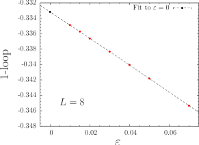
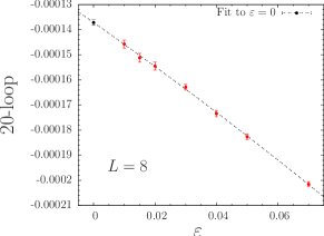
Figure 1: Extrapolation $\varepsilon\rightarrow 0$ for $W_{11}$ for 1-loop (left) and 20-loop (right) for $L=8$.

In Fig. 1 we show the extrapolation $\varepsilon\rightarrow 0$ for lattice size $L=8$ for a plaquette, where we use a general quadratic ansatz in $\varepsilon$ for the fitting function.

We write the general expansion of a Wilson loop of size $N\times M$ in terms of the bare lattice coupling $g$ as

$$W_{NM}=\sum_{n=0}^{20}\,W_{NM}^{(n)}\,g^{2n}\,.$$ (4)

Depending on the loop-size $(N,M)$ we found alternating signs for the perturbative coefficients $W_{NM}^{(n)}$ for smaller $n$ whereas for larger $n$ they turn into a smooth asymptotic behavior. An example is given in Fig. 2 (left) for $L=12$.

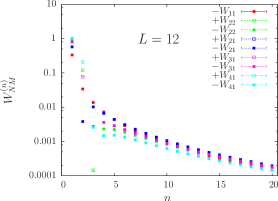
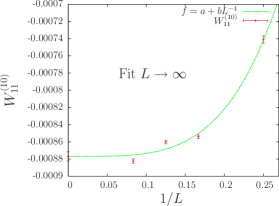
Figure 2: Coefficients for various Wilson loops (left). Extrapolation $L\rightarrow\infty$ for $n=10$ (right).

A typical extrapolation to $L\rightarrow\infty$ for the plaquette is shown on the right side of Fig. 2. Bali [12] has computed one- and two-loop contributions to Wilson loops of various sizes in the standard diagrammatic approach for finite $L$. A comparison of our one- and two-loop NSPT results with his results is given in Table LABEL:BaliTab. Based on the results given by Bali we fixed the functional dependence of the $L\rightarrow\infty$ extrapolation. However, it should be empasized that this extrapolation becomes worse for larger loop sizes $(N,M)$.

Table 1: Comparison of one- and two-loop results for NSPT and standard approach

$W_{NN}$	$L$	NSPT (1-loop)	Bali (1-loop)	NSPT (2-loop)	Bali (2-loop)
$W_{22}$	$4$	$-0.87468(13)$	$-0.87500$	$0.10404(07)$	$0.10406$
	$6$	$-0.90752(12)$	$-0.90762$	$0.11830(10)$	$0.11837$
	$8$	$-0.91164(08)$	$-0.91141$	$0.12008(08)$	$0.11993$
	$12$	$-0.91259(03)$	$-0.91261$	$0.12038(04)$	$0.12038$
$W_{33}$	$6$	$-1.50088(30)$	$-1.50093$	$0.60906(34)$	$0.60866$
	$8$	$-1.52873(23)$	$-1.52803$	$0.63693(23)$	$0.63632$
	$12$	$-1.53526(47)$	$-1.53533$	$0.64370(13)$	$0.64360$
$W_{44}$	$8$	$-2.14128(44)$	$-2.14016$	$1.52351(70)$	$1.52331$
	$12$	$-2.16950(24)$	$-2.16922$	$1.57178(60)$	$1.57006$

3 Perturbative series at large order

The order of perturbation theory we have reached in our calculations allows to study the large order behavior and to test some models concerning the $n-$dependence of the coefficients. This is essential in order to compute the perturbative part of the Wilson loops as precise as possible. In order not to interfere with possible extrapolation ($L\rightarrow\infty$) effects we investigate this for finite $L$.

3.1 Heuristic model

In [13] the authors propose to use a series expansion for a quantity which shows a power-like singularity

$$W_{11}\sim(1-u\,g^{2})^{\gamma}=\sum_{n}\,\frac{\Gamma(n-\gamma)}{\Gamma(n+1)\Gamma(-\gamma)}\,(u\,g^{2})^{n}=\sum_{n}\,c_{n}\,g^{2n}\,.$$ (5)

From (5) one derives the ratio of successive coefficients $c_{n}$ as (slightly modified by a parameter $s$ to account for a small curvature)

$$r_{n}=c_{n}/c_{n-1}=u\left(1-\frac{1+\gamma}{n+s}\right)\,.$$ (6)

In a Domb-Sykes plot - $r_{n}$ plotted against $1/n$ - this is almost a straight line. In Fig. 3 one observes that $r_{n}$ for $W_{11}$ follows this simple functional form almost ideally.

However, the corresponding curves for larger Wilson loops of moderate size have a more pronounced non-linear dependence on $1/n$ as can be seen in Fig. 3.

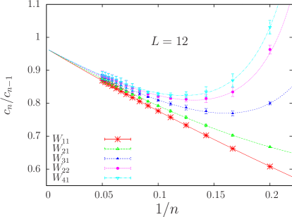
Figure 3: Domb-Sykes plot for various $W_{NM}$ together with their fits (3.3).

This suggests to generalize ansatz (6) by adding an extra power in $n$ (for a detailed discussion see [14])

$$r_{n}=c_{n}/c_{n-1}=u\,\frac{n^{2}+(s-q-1)n+t}{n(n+s)}\,.$$ (7)

For $t=0$ relation (7) is identical to (6). It gives a hyperbola in a Domb-Sykes plot. In this paper we assume that the intercept $u$ has a universal value for all loop sizes $(N,M)$. It is determined from $W_{11}$ which has been computed most precisely. The other parameters $(q,s,t)$ depend on $(N,M)$. The corresponding curves are shown in Fig. 3. They are obtained from the fit ansatz (7) where the parameters are determined in the interval $5\leq n\leq 20$. In this region the perturbative coefficients of the considered Wilson loops show a common asymptotic behaviour as can be seen in Figure 2 (left).

There were speculations that already at order $n=10$ the perturbative coefficients show a factorial growth due to renormalon contributions [4, 6] (for a detailed investigation of this point see also [8]). For the plaquette we plot in Fig. 4 the ratio $r_{n}$ over $n$ for the ansatz (6) (HRS) and the renormalon inspired model as given in [4, 6] (BDMO).

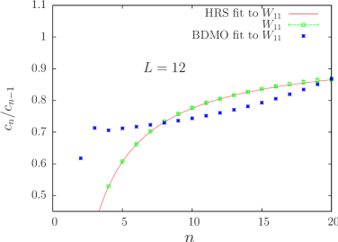
Figure 4: Comparison of $r_{n}$ of the plaquette $W_{11}$ for HRS and BDMO models

We do not observe a factorial growth, at least in the region $n\leq 20$ and for our lattice sizes.

3.2 Boosted perturbation theory

It is well-known that the bare lattice coupling $g$ is a bad expansion parameter due to lattice artefacts like tadpoles. There is a hope that by redefining the coupling $g$ into a boosted coupling $g_{b}$ and the corresponding rearrangement of the series a better convergence behaviour can be achieved. For the plaquette $P=W_{11}$ we use the replacements

$$g^{2}\rightarrow g^{2}_{b}=\frac{g^{2}}{P_{pert,b}}:\quad P_{pert}(g,n^{\star})=1+\sum_{n=1}^{n^{\star}}\,W_{11}^{(n)}\,g^{2n}\rightarrow P_{pert,b}(g_{b},n^{\star})=1+\sum_{n=1}^{n^{\star}}\,W_{b,11}^{(n)}\,g^{2n}_{b}\,,$$ (8)

where $n^{\star}$ is the maximal loop order.

Boosted perturbation theory has been applied to improve the perturbative series for the plaquette for the first time by Rakow [7]. He showed that $P_{pert,b}(g_{b},n^{\star})$ reaches a stable plateau much earlier than $P_{pert}(g,n^{\star})$ as a function of $n^{\star}$.

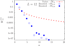
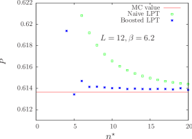
Figure 5: Coefficients for naive and boosted LPT (left). $P$ at $\beta=6.2$ as function of $n^{\star}$ (right).

Fig. 5 (left) shows that the boosted coefficients $W_{b,11}^{(n)}$ oscillate but rapidly become very small. Of course, one should act with caution in the region of $n$ where $|W_{b,11}^{(n)}|\sim 10^{-7}$. The superior convergence behavior for the plaquette is demonstrated in Fig. 5 (right) confirming the result in  [7]. The Monte Carlo result is taken from [15, 16].

4 Non-perturbative gluon condensate

As discussed in the introduction there are speculations whether the difference $\Delta P=P_{pert}-P_{MC}$ behaves as $\sim a^{2}$ or $\sim a^{4}$. We can check this by plotting $\Delta P$ versus $a/r_{0}$ where $r_{0}$ denotes the Sommer scale. The functional relation between $\beta$ and $r_{0}/a$ has been taken from [17]. In Fig. 6 $\Delta P(a/r_{0})$ is plotted in the infinite volume limit ($L\rightarrow\infty$) for both models discussed in the previous sections. The MC data points have been taken from [15, 16]. (The cut-off in the HRS-model data for larger $a$ is due to the convergence radius for the coupling determined by the parameter $u$ in (5).)

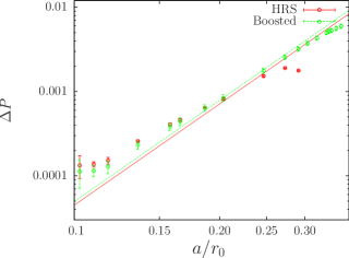
Figure 6: $\Delta P(a/r_{0})$ with fit curves $\sim(a/r_{0})^{4}$.

We make the ansatz $\Delta P(a/r_{0})=C\,(a/r_{0})^{4}$ and approximate $\left(\frac{-b_{0}\,g^{2}}{\beta(g)}\right)\sim 1$. This gives for the range $0.1\leq a/r_{0}\leq 0.25$

$$r_{0}^{4}\,\langle\frac{\alpha}{\pi}G\,G\rangle_{HRS}=1.63(9),\quad r_{0}^{4}\,\langle\frac{\alpha}{\pi}G\,G\rangle_{boosted}=1.80(5).$$ (9)

Fig. 6 shows that the data are well described by the ansatz $\sim(a/r_{0})^{4}$ over a large range of $a$. Inserting , e.g. $r_{0}=0.5$ fm we obtain

$$\langle\frac{\alpha}{\pi}G\,G\rangle_{HRS}=0.039(2)\,GeV^{4},\quad\langle\frac{\alpha}{\pi}G\,G\rangle_{boosted}=0.043(2)\,GeV^{4}\,.$$ (10)

One can try to fit the more general ansatz $\Delta P=C\,(a/r_{0})^{\delta}$ to the data. For the boosted model and $0.1\leq a/r_{0}\leq 0.25$ we get $\delta=3.5\pm 0.1$ which is not too far from $\delta=4$.

All given errors are purely statistical, some of the systematic uncertainties are at least as large, and we are planning a more careful error analysis in the full paper [14]. It should be emphasized that the determination of the gluon condensate depends less on the assumption of large loop order behavior than in earlier investigations where all contributions beyond $n=10$ were obtained by extrapolation.

5 Summary

In this paper we presented the perturbative calculation of Wilson loops of different sizes up to loop order $n=20$ using NSPT. We compared three models to describe the data: a renormalon inspired model (BDMO), a heuristic fit (HRS) and boosted perturbation theory. We found that up to order $n=20$ the resulting curves show a $\sim a^{4}$ behaviour. This supports the claim of Narison and Zakharov [10] that a behaviour $\sim a^{2}$ is due to perturbative series cut a lower order. The values (10) for $\langle\frac{\alpha}{\pi}G\,G\rangle$ found for HRS and boosted PT are larger than obtained in other computations [1, 7, 13]. The gluon condensate can also be obtained from larger and/or asymmetric Wilson loops serving as an additional check. We hope to come back to this problem in [14].

Acknowledgements

This investigation has been supported partly by DFG. H. P. acknowledges useful comments from Y. Meurice. P. R. thanks S. Narison for helpful discussions. We also thank the RCNP at Osaka university for using its NEC SX-9 computer.

References

- [1] M. A. Shifman, A. I. Vainshtein and V. I. Zakharov, Nucl. Phys. B 147 (1979) 385.
- [2] T. Banks, R. Horsley, H. R. Rubinstein and U. Wolff, Nucl. Phys. B 190 (1981) 692; A. Di Giacomo and G. C. Rossi, Phys. Lett B 100 (1981) 481.
- [3] J. Kripfganz, Phys. Lett. B 101 (1981) 169; R. Kirschner, J. Kripfganz, J. Ranft and A. Schiller, Nucl. Phys. B 210 (1982) 567; E.-M. Ilgenfritz and M. Müller-Preussker, Phys. Lett. B 119 (1982) 395.
- [4] G. Burgio, F. Di Renzo, G. Marchesini and E. Onofri, Phys. Lett. B 422 (1998) 219 [arXiv:hep-ph/9706209].
- [5] R. Alfieri, F. Di Renzo, E. Onofri and L. Scorzato, Nucl. Phys. B 578 (2000) 383 [arXiv:hep-lat/0002018].
- [6] F. Di Renzo and L. Scorzato, JHEP 0110 (2001) 038 [arXiv:hep-lat/0011067].
- [7] P. E. L. Rakow, PoS LAT2005 (2006) 284 [arXiv:hep-lat/0510046].
- [8] Y. Meurice, Phys. Rev. D 74 (2006) 096005 [arXiv:hep-lat/0609005].
- [9] J. C. LeGuillou and J. Zinn-Justin, Large-Order Behavior of Perturbation Theory, North-Holland, Amsterdam, 1990.
- [10] S. Narison and V. I. Zakharov, [arXiv:0906.4312[hep-ph]].
- [11] F. Di Renzo and L. Scorzato, JHEP 0410, 073 (2004) [arXiv:hep-lat/0410010].
- [12] G. Bali, private communication.
- [13] R. Horsley, P. E. L. Rakow and G. Schierholz, Nucl. Phys. Proc. Suppl. 106 (2002) 870 [arXiv:hep-lat/0110210].
- [14] E.-M. Ilgenfritz et al., in preparation.
- [15] G. Boyd, J. Engels, F. Karsch, E. Laermann, C. Legeland, M. Lutgemeier and B. Petersson, Nucl. Phys. B 469 (1996) 419 [arXiv:hep-lat/9602007].
- [16] M. Göckeler, R. Horsley, A. C. Irving, D. Pleiter, P. E. L. Rakow, G. Schierholz and H. Stuben, Phys. Rev. D 73 (2006) 014513 [arXiv:hep-ph/0502212].
- [17] S. Necco and R. Sommer, Nucl. Phys. B 622 (2002) 328 [arXiv:hep-lat/0108008].