Dissecting the Gravitational Lens B1608$+$656. II. Precision Measurements of the Hubble Constant, Spatial Curvature, and the Dark Energy Equation of State

Abstract

Strong gravitational lens systems with measured time delays between the multiple images provide a method for measuring the “time-delay distance” to the lens, and thus the Hubble constant. We present a Bayesian analysis of the strong gravitational lens system B1608$+$656, incorporating (i) new, deep Hubble Space Telescope (HST) observations, (ii) a new velocity dispersion measurement of $260\pm 15\rm{\,km\,s^{-1}}$ for the primary lens galaxy, and (iii) an updated study of the lens’ environment. Our analysis of the HST images takes into account the extended source surface brightness, and the dust extinction and optical emission by the interacting lens galaxies. When modeling the stellar dynamics of the primary lens galaxy, the lensing effect, and the environment of the lens, we explicitly include the total mass distribution profile logarithmic slope $\gamma^{\prime}$ and the external convergence $\kappa_{\rm ext}$; we marginalize over these parameters, assigning well-motivated priors for them, and so turn the major systematic errors into statistical ones. The HST images provide one such prior, constraining the lens mass density profile logarithmic slope to be $\gamma^{\prime}=2.08\pm 0.03$; a combination of numerical simulations and photometric observations of the B1608$+$656 field provides an estimate of the prior for $\kappa_{\rm ext}$: $0.10^{+0.08}_{-0.05}$. This latter distribution dominates the final uncertainty on $H_{0}$. Fixing the cosmological parameters at $\Omega_{\rm m}=0.3$, $\Omega_{\rm\Lambda}=0.7$, and $w=-1$ in order to compare with previous work on this system, we find $H_{0}=70.6^{+3.1}_{-3.1}\rm{\,km\,s^{-1}\,Mpc^{-1}}$. The new data provide an increase in precision of more than a factor of two, even including the marginalization over $\kappa_{\rm ext}$. Relaxing the prior probability density function for the cosmological parameters to that derived from the WMAP 5-year data set, we find that the B1608$+$656 data set breaks the degeneracy between $\Omega_{\rm m}$ and $\Omega_{\rm\Lambda}$ at $w=-1$ and constrains the curvature parameter to be $-0.031<\Omega_{\rm k}<0.009$ (95% CL), a level of precision comparable to that afforded by the current Type Ia SNe sample. Asserting a flat spatial geometry, we find that, in combination with WMAP, $H_{0}=69.7^{+4.9}_{-5.0}\rm{\,km\,s^{-1}\,Mpc^{-1}}$ and $w=-0.94^{+0.17}_{-0.19}$ (68% CL), suggesting that the observations of B1608$+$656 constrain $w$ as tightly as do the current Baryon Acoustic Oscillation data.

1. Introduction

The Hubble constant ($H_{0}$, measured in units of $\rm{\,km\,s^{-1}\,Mpc^{-1}}$) is one of the key cosmological parameters since it sets the present age, size, and critical density of the Universe.

Methods for measuring the Hubble constant include Type Ia supernovae (SNe Ia) (e.g. Tammann, 1979; Riess et al., 2009), the Sunyaev-Zel’dovich effect (e.g. Sunyaev & Zel’dovich, 1980; Bonamente et al., 2006), the expanding photosphere method for Type II supernovae (e.g. Kirshner & Kwan, 1974; Schmidt et al., 1994), and maser distances (e.g. Herrnstein et al., 1999; Macri et al., 2006). However, perhaps the two most well-known recent measurements come from the Hubble Space Telescope (HST) Key Project (KP) (Freedman et al., 2001) and the Wilkinson Microwave Anisotropy Probe (WMAP) observations of the cosmic microwave background (CMB) (e.g. Komatsu et al., 2009). The HST KP measurement of $H_{0}$ is based on secondary distance indicators (including Type Ia supernovae, Tully-Fisher, surface brightness fluctuations, Type II supernovae, and the fundamental plane) that are calibrated using Cepheid distances to nearby galaxies with a zero point in the Large Magellanic Cloud. The resulting Hubble constant is $72\pm 8\,\rm{\,km\,s^{-1}\,Mpc^{-1}}$ (Freedman et al., 2001). We note that the largest contributor to the systematic error from the distance ladder of which this measurement depends is the metallicity dependence of the Cepheid period-luminosity relation. More recently, Riess et al. (2009) addressed some of these systematic effects with an improved differential distance ladder using Cepheids, SNe Ia, and the maser galaxy NGC 4258, finding $H_{0}=74.2\pm 3.6\rm{\,km\,s^{-1}\,Mpc^{-1}}$, a 5% local measurement of Hubble’s constant.

The five year measurement made using WMAP temperature and polarization data is $H_{0}=71.9^{+2.6}_{-2.7}\rm{\,km\,s^{-1}\,Mpc^{-1}}$ (Dunkley et al., 2009), under the assumption that the Universe is flat and that the dark energy is described by a cosmological constant (with equation of state parameter $w=-1$). The uncertainty in $H_{0}$ increases markedly if either of these two assumptions is relaxed, due to degeneracies with other cosmological parameters. For example, WMAP gives $H_{0}\sim 50\rm{\,km\,s^{-1}\,Mpc^{-1}}$ without the flatness assumption, and $H_{0}=74^{+15}_{-14}\rm{\,km\,s^{-1}\,Mpc^{-1}}$ for a flat Universe with time-independent $w$ not fixed at $w=-1$. As $H_{0}$ is such an important parameter, it is essential to measure it using multiple methods. In this paper, we use a single strong gravitational lens as an independent probe of $H_{0}$, and explore its systematic errors and relations with other cosmological parameters to provide guidance for future studies. We will show that the single lens is competitive with those of the best current cosmographic probes. Given the current progress in measuring time delays (e.g., Vuissoz et al., 2007, 2008; Paraficz et al., 2009), the methodology in this paper should lead to substantial advances when applied to samples of gravitational lenses.

Strong gravitational lensing occurs when a source galaxy is lensed into multiple images by a galaxy lying along its line of sight. The principle of using strong gravitational lens systems with time-variable sources to measure the Hubble constant is well understood (e.g. Refsdal 1964, Schneider, Kochanek, & Wambsganss 2006). The relative time delays between the multiple images are inversely proportional to $H_{0}$ via a combination of angular diameter distances and depend on the lens potential (mass) distribution. We refer to the combination of angular diameter distances as the “time-delay distance”. By measuring the time delays and modeling the lens potential, one can infer the value for the time-delay distance; this distance-like quantity is primarily sensitive to $H_{0}$ but depends also on other cosmological parameters which must be factored into the analysis. The direct measurement of the time-delay distance means that gravitational lensing is independent of distance ladders.

Despite being an elegant method, gravitational lensing has its limitations. Perhaps the most well-known is the “mass-sheet degeneracy” between $H_{0}$ and external convergence (Falco, Gorenstein, & Shapiro, 1985). There is also a degeneracy between $H_{0}$ and the slope of the lens mass distribution, especially for lenses where the configuration is nearly symmetric (e.g. Wucknitz, 2002). In such cases, the image positions are at approximately the same radial distance from the lens center and so the slope is poorly constrained. In both cases the remedy is to provide more information. Modeling the mass environment of the lens can, in principle, independently constrain the external convergence (e.g., Keeton & Zabludoff 2004; Fassnacht et al. 2006a; Blandford et al. in preparation); likewise, lens galaxy stellar velocity dispersion measurements (e.g., Grogin & Narayan, 1996a, b; Tonry & Franx, 1999; Koopmans & Treu, 2002; Treu & Koopmans, 2002; Barnabè & Koopmans, 2007; McKean et al., 2009) and analysis of any extended images (e.g., Dye & Warren, 2005; Dye et al., 2008) can constrain the mass distribution slope.

A measurement of $H_{0}$ to better than a few percent precision would provide the single most useful complement to results obtained from studies of the CMB for dark energy studies (e.g. Hu, 2005; Riess et al., 2009). Dark energy has been used to explain the accelerating Universe, discovered using luminosity distances to SNe Ia (Riess et al., 1998; Perlmutter et al., 1999). Efforts in studying dark energy often characterize it by a constant equation of state parameter $w$ (where $w=-1$ corresponds to a cosmological constant) and assume a flat Universe. These include Perlmutter et al. (1999), who in their Figure 10 constrained $w\lesssim-0.65$ for present day matter density values of $\Omega_{\rm m}\geq 0.2$, and Eisenstein et al. (2005), who combined their angular diameter distance measurement to $z=0.35$ from Baryon Acoustic Oscillations (BAO) with WMAP data (Spergel et al., 2007) to obtain $w=-0.80\pm 0.18$. Recently, Komatsu et al. (2009) measured $w=-0.992^{+0.061}_{-0.062}$ by combining WMAP 5-year results (WMAP5) with observations of SNe Ia (Kowalski et al., 2008) and BAO (Percival et al., 2007). Komatsu et al. (2009) also explored more general dark energy descriptions. In our study, we combine the time-delay distance measurement from B1608$+$656 with WMAP data to derive a constraint on $w$, and compare the constraining power of B1608$+$656 to that of other cosmographic probes.

In this paper, we present an accurate measurement of $H_{0}$ from the gravitational lens B1608$+$656. A comprehensive lensing analysis of the lens system is in a companion paper (Paper I; Suyu et al. 2009). Using the results from Paper I, we focus in this paper on techniques required to break the mass-sheet degeneracy in order to infer a value of $H_{0}$ with well-understood uncertainty. We then explore the influence of this measurement on other cosmological parameters.

The organization of the paper is as follows. In Section 2, we briefly review the theory behind using gravitational lenses to measure $H_{0}$, include a description of the mass-sheet degeneracy, and describe the dynamics modeling for the measured velocity dispersion. In Section 3, we outline the probability theory for combining various data sets and for including cosmological priors. In Section 4, we present the gravitational lens B1608$+$656 as a candidate for measuring $H_{0}$, and show the lens modeling results. We present the new velocity dispersion measurement and the stellar dynamics modeling in Section 5. The study of the convergence accumulated along the line of sight to B1608$+$656 is discussed in Section 6. The priors for our model parameters are described in Section 7. Finally, in Section 8 we combine the lensing, dynamics and external convergence analyses to break the mass-sheet degeneracy and infer $H_{0}$ from the B1608$+$656 data set. We then show how B1608$+$656 aids in constraining flatness and measuring $w$ when combined with WMAP, before concluding in Section 9.

Throughout this paper, we assume a $w$-CDM universe where dark energy is described by a time-independent equation of state with parameter $w=P/\rho c^{2}$ with present day dark energy density $\Omega_{\rm\Lambda}$, and the present day matter density is $\Omega_{\rm m}$. Each quoted parameter estimate is the median of the appropriate one-dimensional marginalized posterior probability density function (PDF), with the quoted uncertainties showing, unless otherwise stated, the $16^{\rm th}$ and $84^{\rm th}$ percentiles (that is, the bounds of a 68% confidence interval).

2. Measuring $H_{0}$ using lensing, stellar dynamics, and lens environment studies

In this section we briefly review the theory of gravitational lensing for $H_{0}$ measurement (Section 2.1), describe the mass-sheet degeneracy (Section 2.2), and present the dynamics modeling (Section 2.3). Readers familiar with these subjects can proceed directly to Section 3.

2.1. Theory of gravitational lensing

For a strong lens system in an otherwise homogeneous Robertson-Walker universe, the excess time delay of an image at angular position $\vec{\theta}=(\theta_{1},\theta_{2})$ with corresponding source position $\vec{\beta}=(\beta_{1},\beta_{2})$ relative to the case of no lensing is

$$t(\vec{\theta},\vec{\beta})=\frac{1}{c}\frac{D_{\rm d}D_{\rm s}}{D_{\rm ds}}(1+z_{\rm d})\,\phi(\vec{\theta},\vec{\beta}),$$ (1)

where $z_{\rm d}$ is the redshift of the lens, $\phi(\vec{\theta},\vec{\beta})$ is the so-called Fermat potential, and $D_{\rm d}$, $D_{\rm s}$, and $D_{\rm ds}$ are, respectively, the angular diameter distance from us to the lens, from us to the source, and from the lens to the source. The Fermat potential is defined as

$$\phi(\vec{\theta},\vec{\beta})\equiv\left[\frac{(\vec{\theta}-\vec{\beta})^{2}}{2}-\psi(\vec{\theta})\right],$$ (2)

where the first term comes from the geometric path difference as a result of the strong lens deflection, and the second term is the gravitational delay described by the lens potential $\psi(\vec{\theta})$. The scaled deflection angle of a light ray is $\vec{\alpha}(\vec{\theta})=\vec{\nabla}\psi(\vec{\theta})$, and the lens equation that governs the deflection of light rays is $\vec{\beta}=\vec{\theta}-\vec{\alpha}(\vec{\theta})$.

The projected dimensionless surface mass density $\kappa(\vec{\theta})$ is

$$\kappa(\vec{\theta})=\frac{1}{2}\nabla^{2}\psi(\vec{\theta}),$$ (3)

where

$$\kappa(\vec{\theta})=\frac{\Sigma(D_{\rm d}\vec{\theta})}{\Sigma_{\rm cr}}\qquad\mathrm{with}\qquad\Sigma_{\rm cr}=\frac{c^{2}D_{\rm s}}{4\pi GD_{\rm d}D_{\rm ds}},$$ (4)

and $\Sigma(D_{\rm d}\vec{\theta})$ is the physical projected surface mass density.

The constant coefficient in Equation (1) is proportional to the angular diameter distance and hence inversely proportional to the Hubble constant. We can thus simplify Equation (1) to the following:

$$t(\vec{\theta},\vec{\beta}) = \frac{D_{\rm\Delta t}}{c}\,\phi(\vec{\theta},\vec{\beta})$$ (5)

$$\propto \frac{1}{H_{0}}\phi(\vec{\theta},\vec{\beta}),$$ (6)

where $D_{\rm\Delta t}\equiv(1+z_{\rm d})D_{\rm d}D_{\rm s}/D_{\rm ds}$ is referred to as the time-delay distance.

Therefore, by modeling the lens potential ($\psi(\vec{\theta})$) and the source position ($\vec{\beta}$), we can use time-delay lens systems to deduce the value of the Hubble constant, and indeed the other cosmological parameters that appear in $D_{\rm\Delta t}$. In this way, strong lensing can be seen as a kinematic probe of the universal expansion, in the same general category as SNe Ia and BAO. Since the principal dependence of $D_{\rm\Delta t}$ is on $H_{0}$, we continue to discuss lenses as a probe of this one parameter; however, we shall see that the other cosmological parameters play an important role in the analysis.

Gravitational lens systems with spatially extended source surface brightness distributions are of special interest since they provide additional constraints on the lens potential. However, in this case, simultaneous determinations of the source surface brightness and the lens potential are required.

2.2. Mass-sheet degeneracy

We now briefly describe the mass-sheet degeneracy and its relevance to this research (see e.g. Falco et al., 1985; Schneider et al., 2006, for details). As its name suggests, this is a degeneracy in the mass modeling corresponding to the addition of a mass sheet that contributes a convergence and zero shear (and a matching scaling of the original mass distribution) which leaves the predicted image positions unchanged. A circularly symmetric surface mass density distribution that is uniform interior to the line of sight is one example of such a lens. Suppose we have a lens model $\kappa_{\rm model}(\vec{\theta})$ that fits the observables of a lens system (i.e., image positions, flux ratios for point sources, and the image shapes for extended sources). A new model described by the transformation $\kappa_{\rm trans}(\vec{\theta})=\lambda+(1-\lambda)\kappa_{\rm model}(\vec{\theta})$, where $\lambda$ is a constant, would also fit the lensing observables equally well. The parameter $\lambda$ corresponds physically to the convergence of the sheet. Since we might think of including exactly such a parameter to account for additional physical mass lying along the line of sight, or in the lens plane to model a nearby group or cluster, it is clear that the mass-sheet degeneracy corresponds to a degeneracy between this external convergence ($\kappa_{\rm ext}$) and the mass normalization of the lens galaxy.

Despite the invariance of the image positions, shapes and relative fluxes under a mass-sheet transformation, the relative Fermat potential between the images changes according to $\Delta\phi_{\rm trans}(\vec{\theta},\vec{\beta}_{\rm trans})=(1-\lambda)\Delta\phi_{\rm model}(\vec{\theta},\vec{\beta}_{\rm model})$. Therefore, given measured relative time delays $\Delta t$, which are inversely proportional to $H_{0}$ and proportional to the relative Fermat potential (Equation 6), the transformed model $\kappa_{\rm trans}$ would lead to an $H_{0}$ that is a factor $(1-\lambda)$ lower than that of the initial $\kappa_{\rm model}$ (for fixed $\Omega_{\rm m}$, $\Omega_{\rm\Lambda}$, and $w$). In other words, if there is physically any external convergence $\kappa_{\rm ext}$ due to the lens’ local environment or mass structure along the line of sight to the lens system that is not incorporated in the lens modeling, then

$$H_{0}^{\rm{true}}=(1-\kappa_{\rm ext})H_{0}^{\rm{model}}.$$ (7)

This degeneracy is present because lensing observations only deliver relative positions and fluxes. The degeneracy can be broken, allowing us to measure $H_{0}$, if (i) we know the magnitude or angular size of the source in absence of lensing, (ii) we have information on the mass normalization of the lens, or (iii) we can compare the measured shear in the lens with the observed distribution of mass to calibrate $\kappa_{\rm ext}$. For most of the strong lens systems including B1608$+$656, case (i) does not apply, so circumventing the mass-sheet degeneracy requires the input of more information, either about the lensing galaxy itself, or its three-dimensional environment. We distinguish between two kinds of mass sheets: internal and external. Internal mass sheets, which are physically associated with the lens galaxy, are due to nearby, physically associated galaxies, groups or clusters which, crucially, affect the stellar dynamics of the lens galaxy. External mass sheets describe mass distributions that are not physically associated with the lens galaxy and, by definition, do not affect the stellar dynamics. Typically these will lie along the line of sight to the lens (Fassnacht et al., 2006a). We identify $\kappa_{\rm ext}$ as the net convergence of this external mass sheet.

Two methods for breaking the mass-sheet degeneracy are then:

1. Stellar dynamics of the lens galaxy. Stellar dynamics can be used jointly with lensing to break the internal mass-sheet degeneracy by providing an estimate of the enclosed mass at a radius different from the Einstein radius, which is approximately the radius of the lensed images from the lens galaxy (e.g., Grogin & Narayan, 1996a, b; Tonry & Franx, 1999; Koopmans & Treu, 2002; Treu & Koopmans, 2002; Barnabè & Koopmans, 2007). We note that for a given stellar velocity dispersion, there is a degeneracy in the mass and the stellar orbit anisotropy (which characterizes the amount of tangential velocity dispersion relative to radial dispersion). Nonetheless, the mass-isotropy degeneracy is nearly orthogonal to the mass-sheet degeneracy, so a combination of the mass within the effective radius (from the stellar velocity dispersion) and the mass within the Einstein radius (from lensing) effectively breaks both the mass-isotropy and the internal mass-sheet degeneracies. We describe how this works within the context of our chosen mass model in Section 2.3 below.

2. Studying the environment and the line of sight to the lens galaxy. Observations of the field around lens galaxies allow a rough picture of the projected mass distribution to be built up. Many lens galaxies lie in galaxy groups, which can be identified either by their spectra or, more cheaply (but less accurately), by their colors and magnitudes. By modeling the mass distribution of the groups and galaxies in the lens plane and along the line of sight to the lens galaxy, one can estimate the external convergence $\kappa_{\rm ext}$ at the redshift of the lens (e.g. Momcheva et al., 2006; Fassnacht et al., 2006a; Auger et al., 2007, and references therein). The group modeling requires (i) identification of the galaxies that belong to the group of the lens galaxy, and (ii) estimates of the group centroid and velocity dispersion. A number of recipes can be followed. For example, Keeton & Zabludoff (2004) considered two extremes: (i) the group is described by a single smooth mass distribution, and (ii) the masses are associated with individual galaxy group members with no common halo. The realistic mass distribution for a galaxy group should be somewhere between these two extremes. The experience to date is that modeling lens environments accurately is very difficult, with uncertainties of 100% typical (e.g. Momcheva et al., 2006; Fassnacht et al., 2006a). In Section 6, we describe an alternative approach for quantifying the external convergence in a statistical manner: ray-tracing through numerical simulations of large-scale structure (Hilbert et al., 2007). In this section we also present a first attempt at tailoring the ray-tracing results to our one line of sight, using the relative galaxy number counts in the field.

We emphasize that the mass-sheet degeneracy is simply one of the several parameter degeneracies in the lens modeling that has been given a special name. When power-laws ($\kappa\sim bR^{1-\gamma^{\prime}}$, where $R$ is the radial distance from the lens center, $b$ is the normalization of the lens, and $\gamma^{\prime}$ is the radial slope in the mass profile) are used to describe the lens mass distribution, one often finds a $H_{0}$-$\gamma^{\prime}$ degeneracy in addition to the $H_{0}$-$b$-$\kappa_{\rm ext}$ (mass-sheet) degeneracy (for fixed $\Omega_{\rm m}$, $\Omega_{\rm\Lambda}$ and $w$; more generally, $D_{\rm\Delta t}$ would be in place of $H_{0}$). These two degeneracies are of course related via $H_{0}$. The $H_{0}$-$\gamma^{\prime}$ degeneracy primarily occurs in lens systems with symmetric configurations due to a lack of information on $\gamma^{\prime}$. In contrast, lens systems with images spanning a range of radii or with extended images provide information on $\gamma^{\prime}$ (e.g. Wucknitz et al., 2004; Dye et al., 2008), and so the $H_{0}$-$\gamma^{\prime}$ degeneracy is broken. Nonetheless, the $H_{0}$-$b$-$\kappa_{\rm ext}$ degeneracy is still present unless we provide information from dynamics and lens environment studies.

2.3. Stellar dynamics modeling

In order to model the velocity dispersion of the stars in the lens galaxy, we need a model for the local gravitational potential well in which those stars are orbiting. This potential is due to both the mass distribution of the lens galaxy, and also the “internal mass sheet” due to neighboring groups and galaxies physically associated with the lens, as described in the previous subsection. Recent studies such as the Sloan Lens ACS Survey (SLACS) and hydrostatic X-ray analyses found that the sum of these internal components can be well-described by a power law (e.g. Treu et al., 2006; Koopmans et al., 2006; Gavazzi et al., 2007; Koopmans et al., 2009; Humphrey & Buote, 2009). With this in mind, we assume that the total (lens plus sheet) mass density distribution is spherically symmetric and of the form

$$\rho_{\rm local}=\rho_{0}\left(\frac{r_{0}}{r}\right)^{\gamma^{\prime}},$$ (8)

where $\gamma^{\prime}$ is the logarithmic slope of the effective lens density profile, and $\rho_{0}r_{0}^{\gamma^{\prime}}$ is the normalization of the mass distribution that is determined quite precisely by the lensing, up to a small offset contributed by the external convergence $\kappa_{\rm ext}$. This normalization can be expressed in terms of observable or inferrable quantities as we show below.

By integrating $\rho_{\rm local}$ within a cylinder with radius given by the Einstein radius $R_{\rm{Ein}}$, we find

$$M_{\rm local} = 4\pi\int_{0}^{\infty}dz\int_{0}^{R_{\rm{Ein}}}\rho_{0}r_{0}^{\gamma^{\prime}}\frac{s\,{\rm d}s}{(s^{2}+z^{2})^{\gamma^{\prime}/2}}$$ (9)

$$= -\rho_{0}r_{0}^{\gamma^{\prime}}\frac{\pi^{3/2}\Gamma(\frac{\gamma^{\prime}-3}{2})R_{\rm{Ein}}^{3-\gamma^{\prime}}}{\Gamma(\frac{\gamma^{\prime}}{2})}.$$ (10)

However, the mass responsible for creating an Einstein ring is a combination of this local mass and the external mass contributed along the line of sight, so the mass contained within the Einstein ring is

$$M_{\rm Ein}=M_{\rm local}+M_{\rm{ext}}$$ (11)

where $M_{\rm Ein}$ is the mass enclosed within the Einstein radius $R_{\rm{Ein}}$ that would be inferred from lensing, given by

$$M_{\rm Ein}=\pi R_{\rm{Ein}}^{2}\Sigma_{\rm cr},$$ (12)

and $M_{\rm ext}$ is the mass contribution from $\kappa_{\rm ext}$,

$$M_{\rm{ext}}=\pi R_{\rm{Ein}}^{2}\kappa_{\rm ext}\Sigma_{\rm cr}.$$ (13)

Combining Equations (10), (11), (12), and (13), we find

$$\rho_{0}r_{0}^{\gamma^{\prime}}=(\kappa_{\rm ext}-1)\Sigma_{\rm cr}R_{\rm{Ein}}^{\gamma^{\prime}-1}\frac{\Gamma(\frac{\gamma^{\prime}}{2})}{\pi^{1/2}\Gamma(\frac{\gamma^{\prime}-3}{2})}.$$ (14)

Substituting this in Equation (8), we obtain

$$\rho_{\rm local}=(\kappa_{\rm ext}-1)\Sigma_{\rm cr}R_{\rm{Ein}}^{\gamma^{\prime}-1}\frac{\Gamma(\frac{\gamma^{\prime}}{2})}{\pi^{1/2}\Gamma(\frac{\gamma^{\prime}-3}{2})}\frac{1}{r^{\gamma^{\prime}}}.$$ (15)

Spherical Jeans modeling can then be employed to infer the line-of-sight velocity dispersion, $\sigma^{\rm P}(\gamma^{\prime},\kappa_{\rm ext},\beta_{\rm ani},\Omega_{\rm m},\Omega_{\rm\Lambda},w)$, from $\rho_{\rm local}$ by assuming a model for the stellar distribution $\rho_{*}$ (e.g., Binney & Tremaine, 1987). Here, $\beta_{\rm ani}$ is a general anisotropy term that can be expressed in terms of an anisotropy radius parameters for the stellar velocity ellipsoid, $r_{\rm ani}$, in the Osipkov-Merritt formulation (Osipkov, 1979; Merritt, 1985):

$$\beta_{\rm ani}=\frac{r^{2}}{r_{\rm ani}^{2}+r^{2}},$$ (16)

where $r_{\rm ani}=0$ is pure radial orbits and $r_{\rm ani}\rightarrow\infty$ is isotropic with equal radial and tangential velocity dispersions. The dependence of $\sigma^{\rm P}$ on $\Omega_{\rm m}$, $\Omega_{\rm\Lambda}$, and $w$ enters through $\Sigma_{\rm cr}$ and the physical scale radius of the stellar distribution, but the dependence on $H_{0}$ drops out.

We now follow Binney & Tremaine (1987) to show how the model velocity dispersion is calculated. The three-dimensional radial velocity dispersion $\sigma_{\rm r}$ is found by solving the spherical Jeans equation

$$\frac{1}{\rho_{*}}\frac{d(\rho_{*}\sigma_{\rm r})}{dr}+2\frac{\beta_{\rm ani}\sigma_{\rm r}}{r}=-\frac{GM(r)}{r^{2}},$$ (17)

where $M(r)$ is the mass enclosed within a radius $r$ for the total density profile given by Equation (8) and with $\rho_{*}$ given by the Hernquist profile (Hernquist, 1990)

$$\rho_{*}(r)=\frac{{\rm{I_{0}}}a}{2\pi r(r+a)^{3}},$$ (18)

where the scale radius $a$ is related to the effective radius $r_{\rm eff}$ by $a=0.551r_{\rm eff}$ and ${\rm{I_{0}}}$ is a normalization term. The solution to Equation (17) is

$$\sigma_{\rm r}^{2} = \frac{4\pi Ga^{-\gamma^{\prime}}\rho_{0}r_{0}^{\gamma^{\prime}}}{3-\gamma^{\prime}}\frac{r(r+a)^{3}}{r^{2}+r_{\rm ani}^{2}}\cdot$$ (19)

$$\left(\frac{r_{\rm ani}^{2}}{a^{2}}\frac{{\rm{}_{2}F_{1}}[2+\gamma^{\prime},\gamma^{\prime};3+\gamma^{\prime};\frac{1}{1+r/a}]}{(2+\gamma^{\prime})(r/a+1)^{2+\gamma^{\prime}}}+\right.$$

$$\left.\frac{{\rm{}_{2}F_{1}}[3,\gamma^{\prime};1+\gamma^{\prime};-a/r]}{\gamma^{\prime}(r/a)^{\gamma^{\prime}}}\right),$$

where ${\rm{}_{2}F_{1}}$ is a hypergeometric function. The model luminosity-weighted velocity dispersion within an aperture $\mathcal{A}$ is then

$$(\sigma^{\rm P})^{2}=\frac{\int_{\mathcal{A}}[I_{\rm H}(R)\sigma_{\rm s}^{2}*\mathcal{P}]\,R\,{\rm d}R\,{\rm d}\theta}{\int_{\mathcal{A}}[I_{\rm H}(R)*\mathcal{P}]\,R\,{\rm d}R\,{\rm d}\theta},$$ (20)

where $I_{\rm H}(R)$ is the projected Hernquist distribution (Hernquist, 1990), both integrands are convolved with the seeing $\mathcal{P}$ as indicated, and the theoretical (that is, before convolution and integration over the spectrograph aperture) luminosity-weighted projected velocity dispersion $\sigma_{\rm s}$ is given by

$$I_{\rm H}(R)\sigma_{\rm s}^{2}=2\displaystyle\int_{R}^{\infty}(1-\beta_{\rm ani}\frac{R^{2}}{r^{2}})\frac{\rho_{*}\sigma_{\rm r}^{2}r\,{\rm d}r}{\sqrt{r^{2}-R^{2}}}.$$ (21)

The use of a Jaffe (1983) stellar distribution function follows the same derivation.

In the next section, we present the probability theory for obtaining posterior probability distribution of $H_{0}$ by combining the lensing, dynamics and lens environment studies.

3. Probability Theory

We aim to obtain an expression for the posterior probability distribution of cosmological parameters $H_{0}$, $\Omega_{\rm m}$, $\Omega_{\rm\Lambda}$, and $w$ given the various independent data sets of B1608$+$656.

3.1. Notations for joint modeling of data sets

We introduce notations for the observed data and the model parameters that will be used throughout the rest of this paper.

We have three independent data sets for B1608$+$656: the time delay measurements from the radio observations of the four lensed images A, B, C and D (Fassnacht et al., 1999, 2002), HST Advanced Camera for Surveys (ACS) observations associated with program 10158 (PI:Fassnacht; Suyu et al. 2009), and the stellar velocity dispersion measurement of the primary lens galaxy G1 (see Section 5). Let ${\Delta t}$ be the time delay measurements of images A, C and D relative to image B, ${d}$ be the data vector of the lensed image surface brightness measurements of the gravitational lensed image, and $\sigma$ be the stellar velocity dispersion measurement of the lens galaxy.

As shown in Section 2.1, information on $H_{0}$, $\Omega_{\rm m}$, $\Omega_{\rm\Lambda}$, and $w$ comes primarily from the relative time delays between the images, which is a product of the time-delay distance $D_{\rm\Delta t}$ and the Fermat potential difference. The Fermat potential is determined by the lens potential and the source position that is given by the lens equation. Therefore, the first step is to model the lens system using the observed lensed image ${d}$. In order to model the lens mass distribution using the extended source information, we need to model the point-spread function (PSF) ${\mathsf{B}}$, image covariance matrix $\mbox{\boldmath{${\mathsf{C}}$}}_{\mathrm{D}}$, lens galaxy light ${l}$, and dust ${\mathsf{K}}$ (if present) (e.g. Suyu et al., 2009). We collectively denote these discrete models associated with the lensed image processing as $\mbox{\boldmath{${M}$}}_{\rm D}=\{\mbox{\boldmath{${\mathsf{B}}$}},\mbox{\boldmath{${\mathsf{C}}$}}_{\mathrm{D}},\mbox{\boldmath{${l}$}},\mbox{\boldmath{${\mathsf{K}}$}}\}$. We explored a representative subspace of models $\mbox{\boldmath{${M}$}}_{\rm D}$ in Paper I, using the Bayesian evidence from the ACS data analysis to quantify the appropriateness of each model tested. Given a particular image processing model, we can infer the parameters of the lens potential and the source surface brightness distribution from the ACS data ${d}$. The data models are denoted by $\mbox{\boldmath{${M}$}}_{j}=\mbox{\boldmath{${M}$}}_{2},\ldots,\mbox{\boldmath{${M}$}}_{11}$ for Models 2–11 in Paper I.

The lens potential can be simply parametrized by, for example, a singular power-law ellipsoid (SPLE) with surface mass density

$$\kappa(\theta_{1},\theta_{2})=b\left[\theta_{1}^{2}+\frac{\theta_{2}^{2}}{q^{2}}\right]^{(1-\gamma^{\prime})/2},$$ (22)

where $q$ is the axis ratio, $b$ is the lens strength that determines the Einstein radius ($R_{\rm Ein}$), and $\gamma^{\prime}$ is the radial slope (e.g. Barkana, 1998; Koopmans et al., 2003). The distribution is then translated (with two parameters for the centroid position) and rotated by the position angle parameter. There is no need to include an external convergence parameter in the mass distribution during the lens modeling since we cannot determine it due to the mass-sheet degeneracy. Instead, we explicitly incorporate the external convergence in the Fermat potential later on, taking into account the interplay among this parameter, the slope, and the normalization of the effective lens mass distribution. We collectively label all the parameters of the simply-parametrized model by ${\eta}$, except for the radial slope $\gamma^{\prime}$.

Alternatively, the lens potential can be described on a grid of pixels, especially when the source galaxy is spatially extended (which provides additional constraints on the lens potential). We focus on this case; in particular, we decompose the lens potential into an initial simply-parametrized SPLE model $\psi_{0}(\gamma^{\prime},\mbox{\boldmath{${\eta}$}})$ and grid-based potential corrections denoted by the vector ${\delta\psi}$. The final potential, which is on the same grid of pixels as the corrections, is $\mbox{\boldmath{${\psi}$}}=\mbox{\boldmath{${\psi_{0}}$}}(\gamma^{\prime},\mbox{\boldmath{${\eta}$}})+\mbox{\boldmath{${\delta\psi}$}}$, where $\mbox{\boldmath{${\psi_{0}}$}}(\gamma^{\prime},\mbox{\boldmath{${\eta}$}})$ is the vector of initial potential values evaluated at the grid points. Furthermore, we also describe the extended source surface brightness distribution on a (different) grid of pixels by the vector ${s}$. The determination of the source surface brightness distribution given the lens potential model is a regularized linear inversion. The strength and form of the regularization are denoted by $\lambda$ and ${\mathsf{g}}$, respectively. The procedure for obtaining the pixelated potential corrections and the corresponding extended source surface brightness distribution is iterative and is described in detail in Paper I. We highlight that the resulting (iterated) pixelated lens potential model is not limited by the parametrization of the initial SPLE model – tests of this method in Paper I showed that when the iterative procedure converged, the true potential was reconstructed irrespective of the initial model.

The resulting lens potential allows us to compute the Fermat potential $\phi$ at each image position, up to a factor of $(1-\kappa_{\rm ext})$. Combining the Fermat potential with a value of $D_{\rm\Delta t}$ computed given the cosmological parameters {$H_{0}$, $\Omega_{\rm m}$, $\Omega_{\rm\Lambda}$, $w$} provides us with predicted values of the image time delays, $\Delta t^{\rm P}$.

The dynamics modeling of the galaxy is performed following Section 2.3. By construction, the power-law profile for the dynamics modeling with slope $\gamma^{\prime}$ matches the radial profile of the SPLE. Although spherical symmetry is assumed for the dynamics modeling, a suitably defined Einstein radius from the lens modeling leads to $R_{\rm Ein}$ and $M_{\rm Ein}$ that are independent of $q$ and are directly applicable to the spherical dynamics modeling (e.g. Koopmans et al., 2006). Furthermore, the results from SLACS based on spherical dynamics modeling (Koopmans et al., 2009) agree with those from a more sophisticated two-dimensional kinematics analyses of six SLACS lenses (Czoske et al., 2008; Barnabè et al., 2009), indicating that spherical dynamics modeling for B1608+656 is sufficient. The predicted velocity dispersion is dependent on six parameters: 1) the effective lens mass distribution profile slope $\gamma^{\prime}$, 2) the external convergence $\kappa_{\rm ext}$, 3) the anisotropy radius $r_{\rm ani}$, and then the cosmological parameters 4) $\Omega_{\rm m}$, 5) $\Omega_{\rm\Lambda}$, and 6) $w$.

By combining lensing, dynamics, and lens environment studies, we can break the $D_{\rm\Delta t}$-$\kappa_{\rm ext}$ degeneracy to obtain a probability distribution for the cosmological parameters {$H_{0}$, $\Omega_{\rm m}$, $\Omega_{\rm\Lambda}$, $w$} given the data sets. In the inference, we assume that the redshifts of the lens and source galaxies are known exactly for the computation of $D_{\rm\Delta t}$. This is approximately true for B1608$+$656, which has spectroscopic measurements for the redshifts (Myers et al., 1995; Fassnacht et al., 1996) — an uncertainty of $0.0003$ on the redshifts translates to $<0.2\%$ in time-delay distance, and hence $H_{0}$ for fixed $\Omega_{\rm m}$, $\Omega_{\rm\Lambda}$ and $w$. By imposing sensible priors on {$H_{0}$, $\Omega_{\rm m}$, $\Omega_{\rm\Lambda}$, $w$} from other independent experiments such as WMAP5, we can marginalize the distribution to obtain the posterior probability distribution for $H_{0}$.

3.2. Constraining cosmological parameters

In this section, we describe the probability theory for inferring cosmological parameters from the B1608$+$656 data sets. Readable introductions to this type of analysis can be found in the books by Sivia (1996) and MacKay (2003); we use notation consistent with that in Paper I.

Our goal is to obtain the posterior PDF for the model parameters ${\xi}$ given the three independent data sets {${\Delta t}$, ${d}$, $\sigma$}:

$$P(\mbox{\boldmath{${\xi}$}}|\mbox{\boldmath{${\Delta t}$}},\mbox{\boldmath{${d}$}},\sigma)\propto P(\mbox{\boldmath{${\Delta t}$}}|\mbox{\boldmath{${\xi}$}})P(\mbox{\boldmath{${d}$}}|\mbox{\boldmath{${\xi}$}})P(\sigma|\mbox{\boldmath{${\xi}$}})P(\mbox{\boldmath{${\xi}$}}),$$ (23)

where the parameters ${\xi}$ consist of all the model parameters for obtaining the predicted data sets described in Section 3.1: $\gamma^{\prime}$, $\kappa_{\rm ext}$, ${\eta}$, ${\delta\psi}$, ${s}$, $\mbox{\boldmath{${M}$}}_{\rm D}$, $r_{\rm ani}$, $H_{0}$, $\Omega_{\rm m}$, $\Omega_{\rm\Lambda}$, $w$. For notational simplicity, we denote the cosmological parameters as $\mbox{\boldmath{${\pi}$}}=\{H_{0},\Omega_{\rm m},\Omega_{\rm\Lambda},w\}$. In Equation (23), the dependence on $z_{\rm s}$ and $z_{\rm d}$ are implicit.

To obtain the PDF of cosmological parameters ${\pi}$, we marginalize Equation (23) over all parameters apart from ${\pi}$:

$$P(\mbox{\boldmath{${\pi}$}}|\mbox{\boldmath{${\Delta t}$}},\mbox{\boldmath{${d}$}},\sigma) \propto \int{\rm d}\gamma^{\prime}\ {\rm d}\kappa_{\rm ext}\ {\rm d}\mbox{\boldmath{${\eta}$}}\ {\rm d}\mbox{\boldmath{${\delta\psi}$}}\ {\rm d}\mbox{\boldmath{${s}$}}\ {\rm d}\mbox{\boldmath{${M}$}}_{\rm D}\ {\rm d}r_{\rm ani}\cdot$$ (24)

$$\overbrace{P(\mbox{\boldmath{${\Delta t}$}}|\mbox{\boldmath{${\xi}$}})P(\mbox{\boldmath{${d}$}}|\mbox{\boldmath{${\xi}$}})P(\sigma|\mbox{\boldmath{${\xi}$}})}^{\rm likelihood}\cdot$$

$$\overbrace{P(\mbox{\boldmath{${\pi}$}},\gamma^{\prime},\kappa_{\rm ext},\mbox{\boldmath{${\eta}$}},\mbox{\boldmath{${\delta\psi}$}},\mbox{\boldmath{${s}$}},\mbox{\boldmath{${M}$}}_{\rm D},r_{\rm ani})}^{\rm prior}.$$

In the following subsection, we discuss each of the three terms in the joint likelihood function in turn.

3.3. Likelihoods

Each of the three likelihoods in Equation (24) generally depends only on a subset of the parameters ${\xi}$. Specifically, dropping independences, we have $P(\mbox{\boldmath{${\Delta t}$}}|\mbox{\boldmath{${\xi}$}})=P(\mbox{\boldmath{${\Delta t}$}}|\mbox{\boldmath{${\pi}$}},\gamma^{\prime},\kappa_{\rm ext},\mbox{\boldmath{${\eta}$}},\mbox{\boldmath{${\delta\psi}$}},\mbox{\boldmath{${M}$}}_{\rm D})$, $P(\mbox{\boldmath{${d}$}}|\mbox{\boldmath{${\xi}$}})=P(\mbox{\boldmath{${d}$}}|\gamma^{\prime},\mbox{\boldmath{${\eta}$}},\mbox{\boldmath{${\delta\psi}$}},\mbox{\boldmath{${s}$}},\mbox{\boldmath{${M}$}}_{\rm D})$, and $P(\sigma|\mbox{\boldmath{${\xi}$}})=P(\sigma|\Omega_{\rm m},\Omega_{\rm\Lambda},w,\gamma^{\prime},\kappa_{\rm ext},r_{\rm ani})$.

For B1608$+$656, we can simplify and drop independences further in the time delay likelihood $P(\mbox{\boldmath{${\Delta t}$}}|\mbox{\boldmath{${\xi}$}})$ by expressing the relative Fermat potential (relative to image B for the images A, C and D) as

$$\Delta\phi(\gamma^{\prime},\kappa_{\rm ext},\mbox{\boldmath{${M}$}}_{\rm D})=(1-\kappa_{\rm ext})q(\gamma^{\prime},\mbox{\boldmath{${M}$}}_{\rm D}),$$ (25)

and writing the $i^{\rm th}$ (AB, CB or DB) predicted time delay as

$$\Delta t_{i}^{\rm P}=\frac{1}{c}D_{\rm\Delta t}(z_{\rm d},z_{\rm s},\mbox{\boldmath{${\pi}$}})\cdot\Delta\phi_{i}(\gamma^{\prime},\kappa_{\rm ext},\mbox{\boldmath{${M}$}}_{\rm D})$$ (26)

(see Appendix A for details). The resulting likelihood is

$$P(\mbox{\boldmath{${\Delta t}$}}|z_{\rm d},z_{\rm s},\mbox{\boldmath{${\pi}$}},\gamma^{\prime},\kappa_{\rm ext},\mbox{\boldmath{${M}$}}_{\rm D})$$ (27)

$$=\prod_{i=1}^{3}P(\Delta t_{i}|z_{\rm d},z_{\rm s},\mbox{\boldmath{${\pi}$}},\gamma^{\prime},\kappa_{\rm ext},\mbox{\boldmath{${M}$}}_{\rm D}),$$

where we assume that the three time delay measurements are independent, and that each $P(\Delta t_{i}|z_{\rm d},z_{\rm s},\mbox{\boldmath{${\pi}$}},\gamma^{\prime},\kappa_{\rm ext},\mbox{\boldmath{${M}$}}_{\rm D})$ is given by the PDF in Fassnacht et al. (2002).

The pixelated lens potential and source surface brightness reconstruction allows us to compute

$$P(\mbox{\boldmath{${d}$}}|\gamma^{\prime},\mbox{\boldmath{${\eta}$}},\mbox{\boldmath{${\delta\psi}$}}_{\mathrm{MP}},\mbox{\boldmath{${M}$}}_{\rm D}) =\int {\rm d}\mbox{\boldmath{${s}$}}\ P(\mbox{\boldmath{${d}$}}|\gamma^{\prime},\mbox{\boldmath{${\eta}$}},\mbox{\boldmath{${\delta\psi}$}}_{\mathrm{MP}},\mbox{\boldmath{${s}$}},\mbox{\boldmath{${M}$}}_{\rm D})\cdot$$ (28)

$$P(\mbox{\boldmath{${s}$}}|\lambda,\mbox{\boldmath{${\mathsf{g}}$}}),$$

by marginalizing out the source surface brightness ${s}$. The most probable potential correction, $\mbox{\boldmath{${\delta\psi}$}}_{\mathrm{MP}}$, is the result of the pixelated potential reconstruction method. The likelihood for the lens parameters, $P(\mbox{\boldmath{${d}$}}|\gamma^{\prime},\mbox{\boldmath{${\eta}$}},\mbox{\boldmath{${\delta\psi}$}}_{\mathrm{MP}},\mbox{\boldmath{${M}$}}_{\rm D})$, is also the Bayesian evidence of the source surface brightness reconstruction; the analytic expression for this likelihood is given by Equation (19) in Suyu et al. (2006). Part of the marginalization in Equation (24) can be simplified via

$$\int{\rm d}\mbox{\boldmath{${\delta\psi}$}}\ {\rm d}\mbox{\boldmath{${s}$}}\ {\rm d}\mbox{\boldmath{${M}$}}_{\rm D}\ P(\mbox{\boldmath{${d}$}}|\gamma^{\prime},\mbox{\boldmath{${\eta}$}},\mbox{\boldmath{${\delta\psi}$}},\mbox{\boldmath{${s}$}},\mbox{\boldmath{${M}$}}_{\rm D})\cdot$$ (29)

$$\ \ \ \ \ \ P(\mbox{\boldmath{${s}$}}|\lambda,\mbox{\boldmath{${\mathsf{g}}$}})P(\mbox{\boldmath{${M}$}}_{\rm D})P(\mbox{\boldmath{${\delta\psi}$}})$$

$$\propto \sim P(\mbox{\boldmath{${d}$}}|\gamma^{\prime},\mbox{\boldmath{${\eta}$}},\mbox{\boldmath{${M}$}}_{\rm D}=\mbox{\boldmath{${M}$}}_{5}),$$

under various assumptions stated in Appendix A that are either justified in Paper I or will be shown to be valid in Section 4.2. In essence, we find that the ACS data models that give acceptable fits are all equally probable within their errors, making conditioning on $\mbox{\boldmath{${M}$}}_{5}$ (i.e., setting $\mbox{\boldmath{${M}$}}_{\rm D}=\mbox{\boldmath{${M}$}}_{5}$, where $\mbox{\boldmath{${M}$}}_{5}$ is Model 5 in Paper I for the lensed image processing) approximately equivalent to marginalizing over all models $\mbox{\boldmath{${M}$}}_{\rm D}$.

Furthermore, we can marginalize out the parameters of the smooth lens model ${\eta}$ separately:

$$P(\gamma^{\prime}|\mbox{\boldmath{${d}$}},\mbox{\boldmath{${M}$}}_{\rm D}=\mbox{\boldmath{${M}$}}_{5}) \propto \int{\rm d}\mbox{\boldmath{${\eta}$}}\ P(\mbox{\boldmath{${d}$}}|\gamma^{\prime},\mbox{\boldmath{${\eta}$}},\mbox{\boldmath{${M}$}}_{\rm D}=\mbox{\boldmath{${M}$}}_{5})\cdot$$ (30)

$$\ \ P_{\rm no\,ACS}(\gamma^{\prime})\ P(\mbox{\boldmath{${\eta}$}}).$$

(See Appendix A for details of the assumptions involved.) We see that the resulting PDF, $P(\gamma^{\prime}|\mbox{\boldmath{${d}$}},\mbox{\boldmath{${M}$}}_{\rm D}=\mbox{\boldmath{${M}$}}_{5})$, can itself be treated as a prior on the slope $\gamma^{\prime}$. Without the ACS data ${d}$, this distribution will default to the lower level prior $P_{\rm no\,ACS}(\gamma^{\prime})$. For the rest of this section we refer only to the generic prior $P(\gamma^{\prime})$, keeping in mind that this distribution may or may not include the information from the ACS data. This will allow us to isolate the influence of the ACS data on the final results, when we compare the PDF in Equation (30) with some alternative choices of $P(\gamma^{\prime})$.

For the velocity dispersion likelihood, the predicted velocity dispersion $\sigma^{\rm P}$ as a function of the parameters described in Section 3.1 is

$$\sigma^{\rm P}=\sigma^{\rm P}(\Omega_{\rm m},\Omega_{\rm\Lambda},w,\gamma^{\prime},\kappa_{\rm ext},r_{\rm ani}|z_{\rm d},z_{\rm s},r_{\rm eff},R_{\rm Ein}),$$ (31)

where the effective radius, $r_{\rm eff}$, the Einstein radius, $R_{\rm Ein}$, and the mass enclosed within the Einstein radius, $M_{\rm Ein}$, are fixed. The effective radius is fixed by observations, and $R_{\rm Ein}$ and $M_{\rm Ein}$ are the quantities that lensing delivers robustly. The uncertainty in the dynamics modeling due to the error associated with $r_{\rm eff}$, $R_{\rm Ein}$ and $M_{\rm Ein}$ is negligible compared to the uncertainties associated with $\kappa_{\rm ext}$. The likelihood function for $\sigma$ is a Gaussian:

$$P(\sigma|\Omega_{\rm m},\Omega_{\rm\Lambda},w,\gamma^{\prime},\kappa_{\rm ext},r_{\rm ani})$$ (32)

$$=\frac{1}{\sqrt{2\pi\sigma_{\sigma}^{2}}}\exp{\left[-\frac{(\sigma-\sigma^{\rm P})^{2}}{2\sigma_{\sigma}^{2}}\right]}.$$

Finally then, we have the following simplified version of Equation (24), where the posterior PDF has been successfully compartmentalized into manageable pieces:

$$P(\mbox{\boldmath{${\pi}$}}|\mbox{\boldmath{${\Delta t}$}},\mbox{\boldmath{${d}$}},\sigma) \propto \int{\rm d}\gamma^{\prime}\,{\rm d}\kappa_{\rm ext}\,{\rm d}r_{\rm ani}\cdot$$ (33)

$$\ \ \ \ P(\mbox{\boldmath{${\Delta t}$}}|z_{\rm d},z_{\rm s},\mbox{\boldmath{${\pi}$}},\gamma^{\prime},\kappa_{\rm ext},\mbox{\boldmath{${M}$}}_{\rm D}=\mbox{\boldmath{${M}$}}_{5})\cdot$$

$$\ \ \ \ P(\sigma|\Omega_{\rm m},\Omega_{\rm\Lambda},w,\gamma^{\prime},\kappa_{\rm ext},r_{\rm ani})\cdot$$

$$\ \ \ \ P(\gamma^{\prime})\,P(\kappa_{\rm ext})\,P(r_{\rm ani})\,P(\mbox{\boldmath{${\pi}$}}).$$

Sections 4 to 7 address the specific forms of the likelihoods and the priors in Equation (33). In particular, in the next section, we focus on the lens modeling of B1608$+$656 which will justify the assumptions mentioned above and provide both the time delay likelihood and the ACS $P(\gamma^{\prime})$ prior.

4. Lens model of B1608$+$656

The quadruple-image gravitational lens B1608$+$656 was discovered in the Cosmic Lens All-Sky Survey (CLASS) (Myers et al., 1995; Browne et al., 2003; Myers et al., 2003). Figure 1 is an image of B1608$+$656, showing the spatially extended source surface brightness distribution (with lensed images labeled by A, B, C, and D) and two interacting galaxy lenses (labeled by G1 and G2). The redshifts of the source and the lens galaxies are, respectively, $z_{\rm s}=1.394$ (Fassnacht et al., 1996) and $z_{\rm d}=0.6304$ (Myers et al., 1995). We note that the lens galaxies are in a group with all galaxy members in the group lie within $\pm 300\rm{\,km\,s^{-1}}$ of the mean redshift (Fassnacht et al., 2006a). Thus, even a conservative limit of $300\rm{\,km\,s^{-1}}$ for the peculiar velocity of B1608$+$656 relative to the Hubble flow would only change $D_{\rm\Delta t}$ by $0.5\%$. As we will see, this is not significant compared to the systematic error associated with $\kappa_{\rm ext}$. This system is special in that the three relative time delays between the four images were measured accurately with errors of only a few percent: $\Delta t_{\rm AB}=31.5^{+2.0}_{-1.0}\rm{\ days}$, $\Delta t_{\rm CB}=36.0^{+1.5}_{-1.5}\rm{\ days}$, and $\Delta t_{\rm DB}=77.0^{+2.0}_{-1.0}\rm{\ days}$ (Fassnacht et al., 1999, 2002). The additional constraints on the lens potential from the extended source analysis and the accurately measured time delays between the images make B1608$+$656 a good candidate to measure $H_{0}$ with few-percent precision. However, the presence of dust and interacting galaxy lenses (visible in Figure 1) complicate this system. In Paper I, we presented a comprehensive analysis that took into account the extended source surface brightness distribution, interacting galaxy lenses, and the presence of dust for reconstructing the lens potential. In the following subsections, we summarize the data analysis and lens modeling from Paper I, and present the resulting Bayesian evidence values (needed in Equation (30)) from the lens modeling.

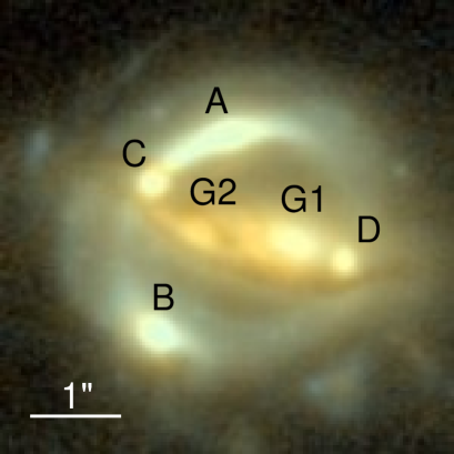
Figure 1.— HST ACS image of B1608$+$656 from 11 orbits in F814W and 9 orbits in F606W. North is up and east is left. The lensed images of the source galaxy are labeled by A, B, C, and D, and the two lens galaxies are G1 and G2. 1 arcsec corresponds to approximately 7 kpc at the redshift of the lens.

4.1. Summary of observations, data analysis, and lens modeling in Paper I

Deep HST ACS observations on B1608$+$656 in F606W and F814W filters were taken specifically to obtain high signal-to-noise ratio images of the lensed source emission.

In Paper I, we investigated a representative sample of PSF, dust, and lens galaxy light models in order to extract the Einstein ring for the lens modeling. Table 1 lists the various PSF and dust models, and we refer the readers to Paper I for details of each model.

The resulting dust-corrected, galaxy-subtracted F814W image allowed us to model both the lens potential and source surface brightness on grids of pixels based on an iterative and perturbative potential reconstruction scheme. This method requires an initial guess potential model that would ideally be close to the true model. In Paper I, we adopt the SPLE1+D (isotropic) model from Koopmans et al. (2003) as the initial model, which is the most up-to-date, simply-parametrized model combining both lensing and stellar dynamics. In the current paper, we additionally investigate the dependence on the initial model by describing the lens galaxies as SPLE models for a range of slopes ($\gamma^{\prime}=1.5,1.6,\ldots,2.5$). Contrary to the SPLE1+D (isotropic) model, the parameters for the SPLE models with variable slopes are constrained by lensing data only, without the velocity dispersion measurement.

The source reconstruction provides a value for the Bayesian evidence, $P(\mbox{\boldmath{${d}$}}|\gamma^{\prime},\mbox{\boldmath{${\eta}$}},\mbox{\boldmath{${\delta\psi}$}},\mbox{\boldmath{${M}$}}_{\rm D})$, which can be used for model comparison (where model refers to the PSF, dust, lens galaxy light, and lens potential model). The reconstructed lens potential (after the pixelated corrections ${\delta\psi}$) for each data model (PSF, dust, lens galaxy light) leads to three estimates of the Fermat potential differences between the image positions. These are presented in the next subsection for the representative set of PSF, dust, lens galaxy light, and pixelated potential model.

4.2. Lens modeling results

In Paper I, we successfully used a pixelated reconstruction method to model small deviations from a smooth lens potential model of B1608$+$656. The resulting source surface brightness distribution is well-localized, and the most probable potential correction $\mbox{\boldmath{${\delta\psi}$}}_{\mathrm{MP}}$ has angular structure approximately following a $\cos\phi$ mode with amplitude $\sim 2\%$. The $\cos 2\phi$ mode, which could mimic an additional external shear or lens mass distribution ellipticity, has a lower amplitude still, indicating that the smooth model of Koopmans et al. (2003) — which includes an external shear of $\simeq 0.08$ — is giving an adequate account of the extended image light distribution. This was the main result of Paper I. The key ingredient in the ACS prior for the lens density profile slope parameter $\gamma^{\prime}$ (Equation (30)) coming from this analysis is the likelihood $P(\mbox{\boldmath{${d}$}}|\gamma^{\prime},\mbox{\boldmath{${M}$}}_{\rm D})$. For a particular choice of slope $\gamma^{\prime}$ and data model $\mbox{\boldmath{${M}$}}_{\rm D}$, this is just the evidence value resulting from the Paper I reconstruction. In this section, our objective is to use the results of this analysis to obtain $P(\gamma^{\prime}|\mbox{\boldmath{${d}$}})$ and $\Delta\phi(\gamma^{\prime},\kappa_{\rm ext})$, marginalizing over a representative sample of data models.

4.2.1 Marginalization of the data model

Table 1 shows the results of the pixelated potential reconstruction at fixed density slope in the initial smooth lens potential model, for various data models $\mbox{\boldmath{${M}$}}_{\rm D}$. Specifically, we used the SPLE1+D (isotropic) model in Koopmans et al. (2003) with $\gamma^{\prime}=2.05$. The uncertainties in the log evidence in Table 1 were estimated as $\sim 0.03\times 10^{4}$ for the log evidence values before potential correction, and $\sim 0.05\times 10^{4}$ for the log evidence values after potential correction.

We see a clear division between models with high and low evidence values, the two groups being separated by a very large factor in probability. Assuming that all the data models $\mbox{\boldmath{${M}$}}_{\rm D}$ are equally probable a priori, the contribution to the marginalized distribution $P(\mbox{\boldmath{${\pi}$}}|\mbox{\boldmath{${\Delta t}$}},\mbox{\boldmath{${d}$}},\sigma)$ (Equation (24)) from these lower-evidence models will be negligible.

The physical difference between these evidence-ranked data models is in the dust correction: the 2-band dust models are found to be less probable than the 3-band dust models. It is useful to quantify the systematic error that would occur with the use of 2-band dust models (which was avoided from the evidence ranking) in terms of the $H_{0}$ value implied by the system. For this simple error estimation we use Equation (5) and assert $\Omega_{\rm m}=0.3$, $\Omega_{\rm\Lambda}=0.7$, $w=-1$ and zero external convergence, as a fiducial reference cosmology (Koopmans et al., 2003). The implied Hubble constants are shown in the final four columns of Table 1. We see that the disfavored use of the 2-band dust maps would have led to values of $H_{0}$ some 15% lower than that inferred from the 3-band maps.

We note that the evidence values of each of the 3-band dust map models $\mbox{\boldmath{${M}$}}_{\rm D}$ are the same within their uncertainties. We can also see that for good data models, specifically $\mbox{\boldmath{${M}$}}_{\rm D}=\mbox{\boldmath{${M}$}}_{5}$, the three $H_{0}$ values have low scatter: these lens models are internally self-consistent. Furthermore, the scatter between the values for the different good data models is also low: the high evidence data models consistently return the same Hubble constant. This is the basis for the approximations (in Section 3.3 and Appendix A) that the likelihood $P(\mbox{\boldmath{${\Delta t}$}}|\mbox{\boldmath{${\xi}$}})$ is effectively constant with the 3-band dust map models $\mbox{\boldmath{${M}$}}_{\rm D}$. Assuming that we have indeed obtained the optimal set of $\mbox{\boldmath{${M}$}}_{\rm D}$, we can approximate the likelihoods in Equations (30) and (33) as being evaluated for model $\mbox{\boldmath{${M}$}}_{5}$.

4.2.2 Effects of the potential corrections

Having approximately marginalized out $\mbox{\boldmath{${M}$}}_{\rm D}$ by conditioning on $\mbox{\boldmath{${M}$}}_{5}$, we now consider the impact of the potential corrections discussed in Paper I. In particular, we seek the likelihood for the density profile slope parameter $\gamma^{\prime}$, $P(\mbox{\boldmath{${d}$}}|\gamma^{\prime}=\gamma^{\prime}_{i},\mbox{\boldmath{${\eta}$}},\mbox{\boldmath{${\delta\psi}$}}_{\mathrm{MP}},\mbox{\boldmath{${M}$}}_{\rm D}=\mbox{\boldmath{${M}$}}_{5})$. We characterize this function on a grid of slope values in the range of $\gamma^{\prime}=1.5,1.6\ldots,2.5$, first re-optimizing the parameters of the smooth lens model, and then computing the source reconstruction evidences both with and without potential correction. These are tabulated in Table 2. We again compute the Fermat potential differences and implied Hubble constant values as before.

The spread of the three implied $H_{0}$ values at fixed density slope is again small: we conclude that the internal self-consistency of the lens model depends on the data model but not $\gamma^{\prime}$. The table also shows that the smooth SPLE model provides a good estimate of the relative Fermat potentials. Indeed, this was the principal conclusion of Paper I. The relative thickness of the arcs is sensitive to the SPLE density profile slope $\gamma^{\prime}$, as can be seen in the first two columns of Table 2: the evidence clearly favors $\gamma^{\prime}\simeq 2.05$, as previously found by Koopmans et al. (2003). Indeed, exponentiating this gives quite a sharply peaked function, which we return to below.

How is the potential correction then affecting the model? In Table 2 we can see that the corrected potential leads to nearly the same evidence value ($P(\mbox{\boldmath{${d}$}}|\gamma^{\prime}=\gamma^{\prime}_{i},\mbox{\boldmath{${\eta}$}},\mbox{\boldmath{${\delta\psi}$}}_{\mathrm{MP}},\mbox{\boldmath{${M}$}}_{\rm D}=\mbox{\boldmath{${M}$}}_{5})$) for a wide range of underlying density slopes, and yet barely changes the relative Fermat potential values. The unchanging nature of the Fermat potential is due to the curvature type of regularization on the potential corrections suppressing the addition of mass within the potential reconstruction annulus. From Kochanek (2002), the relative Fermat potential depends only on the mean surface mass density enclosed in the annulus between the images, to first order in $\delta R/\langle R\rangle$, where $\delta R$ is the difference in the radial distance of the image locations from the effective center of the lens galaxies and $\langle R\rangle$ is the mean radius of the images. The mean surface mass density depends on the slope of the initial SPLE model (hence the trend we see in relative Fermat potential in the left-hand side of Table 2), but not on the potential corrections due to the curvature regularization imposed. Therefore, to first order in $\delta R/\langle R\rangle$, the Fermat potential depends only indirectly on $\gamma^{\prime}$ via the mean surface mass density. The second order term is very small — it has a prefactor of 1/12 and for B1608$+$656, $(\delta R/\langle R\rangle)^{2}\sim 0.1$. Therefore, for good and self-consistent data models, the potential corrections $\mbox{\boldmath{${\delta\psi}$}}_{\mathrm{MP}}$ do not change the Fermat potential significantly.

The right-hand side of Table 2, where a wide range of initial slope values provide good fits to the data, is therefore effectively a manifestation of the mass-sheet degeneracy. One can understand the effect of the potential corrections as making local corrections to the effective density profile slope in order to fit the ACS data. The change in slope by the pixelated corrections would create a deficit/surplus of mass in the annulus, which the pixelated potential corrections then add/subtract back into the annulus in the form of a constant mass sheet to (i) enforce the prior (no net addition of mass within annulus) and (ii) continue to fit the arcs equally well.

We conclude that the value of the potential correction analysis is in demonstrating that the double SPLE model for B1608$+$656 is, despite the system’s complexity, a good model for the high fidelity HST data. The corrections are small in magnitude ($\simeq 2\%$ relative to the initial SPLE model), and the inclusion of the ${\delta\psi}$ neither significantly reduces the dispersion in implied $H_{0}$ values between the image pairs, nor alters the rank order of the data models. We therefore use the information on the slope of the initial SPLE model from the ACS data without potential corrections, thus using the information on the relative thickness of the lensed extended images clearly present. How we derive our estimate for $P(\mbox{\boldmath{${d}$}}|\gamma^{\prime},\mbox{\boldmath{${M}$}}_{\rm D})$ from column 2 of Table 2 is described next.

Table 1 log evidence values and relative Fermat potential values before and after the pixelated potential reconstruction for various data models with the SPLE1+D (isotropic) initial model

Data Model			Initial Potential	Corrected Potential
Model	PSF	dust	log P	log P	$\Delta\phi^{\rm{AB}}$	$\Delta\phi^{\rm{CB}}$	$\Delta\phi^{\rm{DB}}$	$H_{0}^{\rm{AB}}$	$H_{0}^{\rm{CB}}$	$H_{0}^{\rm{DB}}$	$\bar{H_{0}}$
			$(\times 10^{4})$	$(\times 10^{4})$
5	B1	3-band	$1.56$	$1.77$	0.244	0.279	0.575	78.1	78.1	75.1	$77.1\pm 1.7$
9	C	B1/3-band	$1.56$	$1.76$	0.240	0.280	0.563	76.7	78.3	73.5	$76.2\pm 2.4$
3	C	3-band	$1.60$	$1.76$	0.243	0.277	0.570	77.6	77.5	74.4	$76.5\pm 1.8$
2	drz	3-band	$1.48$	$1.75$	0.238	0.278	0.548	76.0	77.7	71.6	$75.1\pm 3.1$
7	B2	3-band	$1.55$	$1.75$	0.237	0.274	0.571	75.7	76.7	74.6	$75.7\pm 1.0$
11	B1	no dust	$1.27$	$1.72$	0.229	0.263	0.576	73.2	73.6	75.3	$74.0\pm 1.1$
10	B1	C/2-band	$1.36$	$1.61$	0.193	0.227	0.565	61.8	63.5	73.8	$66.4\pm 6.4$
4	C	2-band	$1.40$	$1.58$	0.199	0.234	0.560	63.6	65.6	73.1	$67.4\pm 5.0$
6	B1	2-band	$1.10$	$1.41$	0.196	0.226	0.559	62.5	63.2	73.0	$66.2\pm 5.8$
8	B2	2-band	$1.23$	$1.40$	0.201	0.234	0.556	64.3	65.4	72.7	$67.4\pm 4.5$
				$\Delta\phi$ and $H_{0}$ values from initial SPLE1+D (isotropic)
					0.243	0.271	0.575	77.7	75.8	75.1	$76.2\pm 1.3$

Notes — The uncertainties in the log evidence before and after the potential corrections are $\sim 0.03\times 10^{4}$ and $\sim 0.05\times 10^{4}$, respectively. The relative Fermat potentials are in units of ${\rm arcsec}^{2}$, and the $H_{0}$ values are in units of $\rm{\,km\,s^{-1}\,Mpc^{-1}}$. The $\bar{H_{0}}$ values are the mean and standard deviation from the mean of the three estimates obtained using the initial/corrected potential and the three time delays, without taking into account the uncertainties associated with the time delays. These $H_{0}$ values assume $\Omega_{\rm m}=0.3$, $\Omega_{\rm\Lambda}=0.7$ and $w=-1$, and are listed purely to aid the digestion of the $\Delta\phi$ values. The full analysis for obtaining the probability distribution for the cosmological parameters is described in Section 8.

Table 2 log evidence value before and after the pixelated potential reconstruction for initial models with various slope using PSF-B1 and the 3-band dust map ($\mbox{\boldmath{${M}$}}_{\rm D}$=Model 5)

	Initial Potential								Corrected Potential
$\gamma^{\prime}$	log P	$\Delta\phi^{\rm{AB}}$	$\Delta\phi^{\rm{CB}}$	$\Delta\phi^{\rm{DB}}$	$H_{0}^{\rm{AB}}$	$H_{0}^{\rm{CB}}$	$H_{0}^{\rm{DB}}$	$\bar{H_{0}}$	log P	$\Delta\phi^{\rm{AB}}$	$\Delta\phi^{\rm{CB}}$	$\Delta\phi^{\rm{DB}}$	$H_{0}^{\rm{AB}}$	$H_{0}^{\rm{CB}}$	$H_{0}^{\rm{DB}}$	$\bar{H_{0}}$
	($\times 10^{4}$)								($\times 10^{4}$)
1.5	1.38	0.125	0.139	0.287	40.2	39.0	37.6	$38.9\pm 1.3$	1.73	0.130	0.143	0.290	41.7	40.2	38.0	$39.9\pm 1.9$
1.6	1.48	0.147	0.163	0.338	47.2	45.8	44.3	$45.7\pm 1.4$	1.77	0.150	0.170	0.349	48.1	47.6	45.6	$47.1\pm 1.3$
1.7	1.52	0.174	0.193	0.403	55.5	54.0	52.7	$54.0\pm 1.4$	1.75	0.178	0.201	0.417	57.0	56.2	54.5	$55.9\pm 1.3$
1.8	1.54	0.190	0.211	0.442	60.8	59.1	57.7	$59.2\pm 1.5$	1.77	0.194	0.215	0.457	61.9	60.2	59.7	$60.7\pm 1.2$
1.9	1.58	0.210	0.234	0.491	67.1	65.4	64.1	$65.6\pm 1.4$	1.76	0.210	0.237	0.510	67.3	66.4	66.6	$66.8\pm 0.5$
2.0	1.60	0.229	0.256	0.540	73.3	71.6	70.5	$71.8\pm 1.3$	1.79	0.231	0.261	0.549	73.8	73.0	71.7	$72.9\pm 1.1$
2.1	1.60	0.247	0.276	0.586	79.0	77.3	76.6	$77.6\pm 1.2$	1.79	0.250	0.287	0.606	80.0	80.1	79.1	$79.8\pm 0.5$
2.2	1.58	0.264	0.296	0.632	84.5	82.8	82.6	$83.3\pm 1.0$	1.77	0.258	0.299	0.648	82.5	83.7	84.6	$83.7\pm 1.1$
2.3	1.57	0.281	0.315	0.676	89.8	88.0	88.3	$88.7\pm 0.9$	1.79	0.267	0.311	0.678	85.3	86.9	88.5	$86.9\pm 1.6$
2.4	1.55	0.297	0.332	0.720	94.8	92.8	94.0	$93.9\pm 1.0$	1.79	0.299	0.344	0.738	95.6	96.3	96.4	$96.2\pm 0.4$
2.5	1.49	0.312	0.348	0.763	99.8	97.4	99.6	$98.9\pm 1.3$	1.78	0.311	0.357	0.759	99.4	99.7	99.1	$99.5\pm 0.3$

Notes — notation and uncertainties are the same as those described in the notes for Table 1.

4.2.3 The ACS posterior PDF for $\gamma^{\prime}$

In the previous section, we explored the HST data constraints on the slope parameter, optimizing the other parameters of the SPLE lens model at each step. To characterize properly $P(\gamma^{\prime}|\mbox{\boldmath{${d}$}},\mbox{\boldmath{${M}$}}_{\rm D}=\mbox{\boldmath{${M}$}}_{5})$ in Equation (30), we would need to marginalize over all lens parameters ${\eta}$ instead. However, as we shall now see, this optimization approximation is actually a good one and is certainly the most tractable solution due to the high dimensionality of the problem (16 parameters to describe G1, G2 and external shear). Direct sampling in the 16-dimensional parameter space of $P(\mbox{\boldmath{${d}$}}|\gamma^{\prime},\mbox{\boldmath{${\eta}$}},\mbox{\boldmath{${M}$}}_{\rm D}=\mbox{\boldmath{${M}$}}_{5})\,P_{\rm no\,ACS}(\gamma^{\prime})\,P(\mbox{\boldmath{${\eta}$}})$ in Equation (30) via, for example, Markov chain Monte Carlo (MCMC) techniques using the extended source information is not feasible on a reasonable time scale. Importance sampling of the prior PDF from the radio data of image positions and fluxes ($P_{\rm no\,ACS}(\gamma^{\prime},\mbox{\boldmath{${\eta}$}})=P_{\rm no\,ACS}(\gamma^{\prime},\mbox{\boldmath{${\eta}$}}|{\rm radio})$) by weighing the samples by $P(\mbox{\boldmath{${d}$}}|\gamma^{\prime},\mbox{\boldmath{${\eta}$}},\mbox{\boldmath{${M}$}}_{\rm D}=\mbox{\boldmath{${M}$}}_{5})$ is difficult since $\gamma^{\prime}$ is effectively unconstrained by the radio data (the $\chi^{2}$ changes by $\lesssim 1$ in the slope range between 1.5 and 2.5).

It is precisely the unconstrained nature of the $\gamma^{\prime}$ parameter that makes the optimization approximation so good. The “tube” of $\gamma^{\prime}$-degeneracy traversing the 16-dimensional parameter space dominates the uncertainties in the parameters. We thus assume that the tube of $\gamma^{\prime}$-degeneracy has negligible thickness (a degeneracy curve), and use $P(\mbox{\boldmath{${d}$}}|\gamma^{\prime},\mbox{\boldmath{${\eta}$}},\mbox{\boldmath{${M}$}}_{\rm D}=\mbox{\boldmath{${M}$}}_{5})$ to break the degeneracy. Specifically, we use the radio observations, HST Near Infrared Camera and Multi-Object Spectrometer 1 (NICMOS) images (Proposal 7422; PI:Readhead), and time delay data to obtain the best-fitting $\hat{\mbox{\boldmath{${\eta}$}}}$ for a given $\gamma^{\prime}$=$\gamma^{\prime}_{i}$ (assuming $\Omega_{\rm m}=0.3$, $\Omega_{\rm\Lambda}=0.7$ and $w=-1$ in using the time delay data), and compute the corresponding $P(\mbox{\boldmath{${d}$}}|\gamma^{\prime}_{i},\hat{\mbox{\boldmath{${\eta}$}}},\mbox{\boldmath{${M}$}}_{\rm D}=\mbox{\boldmath{${M}$}}_{5})$. These are the listed evidence values in the second column of Table 2 for the various $\gamma^{\prime}_{i}$ values. The time delay data are included because the predicted relative Fermat potential among the image pairs using the radio and NICMOS data are otherwise inconsistent with one another. The optimized parameters from only the radio and NICMOS data lead to $\chi^{2}\sim 600$ for just the time delay data; including the time delay data reduces the time delay $\chi^{2}$ to $\sim 1$ with only a mild increase in the radio and NICMOS $\chi^{2}$ of $\sim 6$. We “undo” the inclusion of the time delay data (so that we do not use the time delay data twice in the importance sampling of Equation (33)) by subtracting the log likelihood of the time delay from the log likelihood of ${d}$; the effect is negligible since the latter is $\sim 10^{4}$ higher in magnitude.

Our thin degeneracy tube assumption implies that $P(\mbox{\boldmath{${d}$}}|\gamma^{\prime})\simeq P(\mbox{\boldmath{${d}$}}|\gamma^{\prime},\hat{\mbox{\boldmath{${\eta}$}}})$, such that the posterior PDF for the slope is $P(\gamma^{\prime}|\mbox{\boldmath{${d}$}})\propto P(\mbox{\boldmath{${d}$}}|\gamma^{\prime})\ P_{\rm no\,ACS}(\gamma^{\prime})$. Assigning a uniform prior (i.e., $P_{\rm no\,ACS}(\gamma^{\prime})$ is constant), we arrive at the result that our desired PDF is just the exponentiation of the log evidence in column 2 of Table 2. Fitting these log evidences with the following quadratic function,

$$\log P(\gamma^{\prime}|\mbox{\boldmath{${d}$}})=C-\frac{(\gamma^{\prime}-\gamma^{\prime}_{0})^{2}}{2\sigma_{\gamma^{\prime}}^{2}},$$ (34)

we obtain the following best-fit parameter values: $\gamma^{\prime}_{0}=2.081\pm 0.027$, $\sigma_{\gamma^{\prime}}=0.0091\pm 0.0008$, and $C=(1.60\pm 0.01)\times 10^{4}$. While the PDF width $\sigma_{\gamma^{\prime}}$ is very small, the centroid is not well determined. Adding $\sigma_{\gamma^{\prime}}$ and the uncertainty in $\gamma^{\prime}_{0}$ in quadrature, we finally approximate $P(\gamma^{\prime}|\mbox{\boldmath{${d}$}})$ with a Gaussian centered on $2.08$ with standard deviation $0.03$. This provides the prior on $\gamma^{\prime}$ from the ACS data (in Equation (33)).

The deep ACS data therefore allow a significant improvement to the previous measurement in Koopmans et al. (2003) of $\gamma^{\prime}=1.99\pm 0.20$, which was based on the radio data and the NICMOS ring. Coincidentally, our $\gamma^{\prime}=2.08\pm 0.03$ is identical, apart from the spread, to the measurement from SLACS of $\gamma^{\prime}=2.08\pm 0.2$ that was based on a sample of massive elliptical lenses (Koopmans et al., 2009). The spread of 0.2 in the SLACS measurement is the intrinsic scatter of slope values in the sample, and is larger than the typical uncertainties associated with individual systems in the sample of $\sim 0.15$. We note that our measurement is not the first percent-level determination of a strong lens density profile slope. Wucknitz et al. (2004) used high precision astrometric measurements from VLBI data to constrain the $\gamma^{\prime}$ parameter in B0218$+$357 to be $1.96\pm 0.02$ (where we have transformed their $\beta$ into our notation). However, they did not use exactly the same model as we do here (instead working with combinations of isothermal elliptical potentials and neglecting external convergence). Dye & Warren (2005) measured the power-law slope of the lens galaxy in the Einstein ring system 0047-2808 to be $\gamma^{\prime}=2.11\pm 0.04$ based on the extended image constraints. More recently, Dye et al. (2008) determined the power-law slope of the extremely massive and luminous lens galaxy in the Cosmic Horseshoe Einstein ring system J1004+4112 to be $\gamma^{\prime}=1.96\pm 0.02$.

4.2.4 Predicted relative Fermat potentials

In order to be able to calculate the time delay likelihood function, $P(\mbox{\boldmath{${\Delta t}$}}|z_{\rm d},z_{\rm s},\mbox{\boldmath{${\pi}$}},\gamma^{\prime},\kappa_{\rm ext},\mbox{\boldmath{${M}$}}_{\rm D})$, at any value of the slope $\gamma^{\prime}$, we need to interpolate the Fermat potential differences given in Table 2. In fact, these data give us the function $q(\gamma^{\prime})$ to insert into Equation (25): we can do the interpolation at $\kappa_{\rm ext}=0.0$ and then rescale by $(1-\kappa_{\rm ext})$ without loss of generality.

For each of the image pairs, we fit the relative Fermat potential difference as a third-order polynomial function of $\gamma^{\prime}$ using the values we have at the discrete points $\gamma^{\prime}_{i}$ for the SPLE models in the table. Recall that the SPLE model provides an unbiased estimate of the relative Fermat potential, and that the various top data models $\mbox{\boldmath{${M}$}}_{\rm D}$ gave consistent estimates. Thus, the polynomial fit gives the function $q(\gamma^{\prime},\mbox{\boldmath{${M}$}}_{\rm D})$ in Equation (25). The third-order polynomial fit leads to residuals ($=(\Delta\phi_{i}-\Delta\phi^{\rm poly})/(\Delta\phi_{i})$) of $<1\%$ for all image pairs at all slope points in Table 2 except for $\gamma^{\prime}_{i}=1.7$, which has residuals of $\sim 2\%$.

5. Breaking the Mass-Sheet Degeneracy: Stellar Dynamics

In this section, we present the observations and data reduction for measuring the velocity dispersion $\sigma$ of G1 in B1608$+$656. This measurement appears as the likelihood function given in Equation (32) above.

5.1. Observations

We have obtained a high signal-to-noise spectrum of B1608$+$656 using the Low-Resolution Imaging Spectrometer (LRIS; Oke et al. 1995) on Keck 1. The data were obtained from the red side of the spectrograph on 12 June 2007 using the 831/8200 grating with the D680 dichroic in place. A slit mask was employed to obtain simultaneously spectra for two additional strong lenses in the field (Fassnacht et al., 2006b) and to continue to probe the structure along the line of sight to the lens (Fassnacht et al., 2006a). The night was clear with a nominal seeing of 0$\farcs$9, and 10 exposures of 1800s and one exposure of 600s were obtained for a total exposure time of 18600s.

Each exposure was reduced individually using a custom pipeline (see Auger et al., 2008, for details) that performs a single resampling of the spectra onto a constant wavelength grid; the same wavelength grid was used for all exposures to avoid resampling the spectra when combining them, and an output pixel scale of 0.915 Å was used to match the dispersion of the 831/8200 grating. Individual spectra were extracted from an aperture 0$\farcs$84 wide (corresponding to 4 pixels on the LRIS red side) centered on the peak of the flux of the lensing galaxy G1. The size of the aperture was chosen to avoid contamination from the spectrum of G2 while maximizing the total flux for an improved signal-to-noise ratio. The extracted spectra were combined by clipping the extreme points at each wavelength and taking the variance-weighted sum of the remaining data points. The same extraction and coaddition scheme was performed for a sky aperture to determine the resolution of the output co-added spectrum; we find the resolution to be ${\rm R}=2560$, corresponding to $\sigma_{\rm obs}=49.7\,{\rm km\,s^{-1}}$. The signal-to-noise ratio per pixel of the final spectrum is $\sim 60$.

5.2. Velocity dispersion measurement

We use a Python-based implementation of the velocity-dispersion code from van der Marel (1994), with one important modification. Our implementation allows for a linear sum of template spectra to be modeled using a bounded variable least squares solver with the constraint that each template must have a non-negative coefficient. We use a set of templates from the INDO-US stellar library containing spectra for a set of seven K and G giants with a variety of temperatures and spectra for an F2 and an A0 giant. These templates of early-type stars are particularly important for B1608$+$656, which has a post-starburst spectrum (Myers et al., 1995).

We perform our modeling over a wide range of wavelength intervals and find a stable solution over a variety of spectral features; we therefore choose to use the rest-frame range from 4200 Å to 4900 Å for our fit. The INDO-US templates have a constant-wavelength resolution of 1.2 Å which corresponds to $\sigma_{\rm template}=33.6\rm{\,km\,s^{-1}}$ over this wavelength range. We iterate over a range of template combinations and polynomial continuum orders and find that a variety of solutions that vary around $260\,{\rm km\,s^{-1}}$ with a spread of about $13\,{\rm km\,s^{-1}}$ and statistical uncertainties of $7.7\,{\rm km\,s^{-1}}$ (see Figure 2). We therefore adopt a velocity dispersion of $\sigma=260\pm 15\rm{\,km\,s^{-1}}$, with the error incorporating the systematic template mismatch and the statistical error for the models. This agrees with the previous measurement of $\sigma_{\rm ap}=247\pm 35\rm{\,km\,s^{-1}}$ by Koopmans et al. (2003) with a significant reduction in the uncertainties, though we note that the two velocity dispersions have been measured in slightly different apertures.

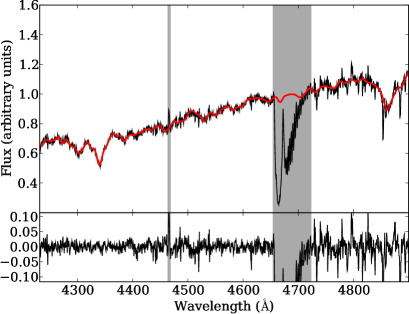
Figure 2.— The LRIS spectrum of B1608$+$656 (black line) with a model generated from all 9 INDO-US templates and a 9th order continuum overplotted (red line). The gray shaded areas were not included in the fit, and the lower panel shows the fit residuals. The spectrum and our modeling suggest a central velocity dispersion of $\sigma=260\pm 15\,{\rm km\,s^{-1}}$, including systematic errors.

6. Breaking the Mass-Sheet Degeneracy: Lens Environment

In this section, we outline two approaches for quantifying the prior probability distributions of the external mass sheet $\kappa_{\rm ext}$. Computing this quantity such that Equation (7) holds true is not a trivial matter. The non-linearity of strong lensing means that the surface mass density at a given angular position in successive redshift planes between the observer and the source cannot simply be scaled by the appropriate distance ratios and summed: rather, the deflection angles (which can be large) need to be taken into account when calculating the distortion matrices (which contain and define the external convergence and shear), leading us towards a ray-tracing approach (Hilbert et al., 2009). Detailed investigation of the ray paths down the B1608$+$656 light cone is beyond the scope of this paper, and we defer it to a later work (Blandford et al. in preparation). In this section we use the statistics of B1608$+$656-like fields in numerical simulations to derive a PDF for $\kappa_{\rm ext}$.

6.1. Ray-tracing through the Millennium Simulation

Following Hilbert et al. (2007), we use the multiple-lens-plane algorithm to trace rays through the Millennium Simulation (MS; Springel et al., 2005), one of the largest N-body simulations of cosmic structure formation. We then identify lines of sight where strong lensing by matter structures at $z_{\rm d}=0.63$ occurs for sources at $z_{\rm s}=1.39$. The convergence along these lines of sight is estimated by summing the projected matter density on the lens planes weighted for a source at $z_{\rm s}=1.39$⁹ along the ray trajectory. By excluding the primary lens plane at $z_{\rm d}=0.63$ that causes the strong lensing, the constructed convergence is truly external to the lens and is due to the line-of-sight contributions only. By sampling many lines of sight, we obtain an estimate for the probability density function of $\kappa_{\rm ext}$ from simulations. We denote this as the “MS” prior on $\kappa_{\rm ext}$.

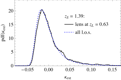
Figure 3.— Probability distribution for the external convergence $\kappa_{\mathrm{ext}}$ along strongly lensed lines of sight from the Millennium Simulation for the lens redshift $z_{\mathrm{L}}$ and source redshifts $z_{\mathrm{S}}$ of B1608$+$656 (solid line) compared to the convergence distribution for all lines of sight (dotted line).

Figure 3 shows the predicted amount of external convergence constructed using $6.4\times 10^{8}$ lines of sight (with and without strong lenses) to sources at $z_{\rm s}=1.39$: of these, $8.0\times 10^{3}$ lines of sight contain strong lenses. For both curves, the mean $\kappa_{\rm ext}$ is consistent with zero with a spread of $\sim 0.04$.

How should we interpret this distribution? According to its definition, $\kappa_{\rm ext}$ could have contributions from galaxies on the primary lens plane that do not affect the dynamics. Neglecting these contributions (effectively assuming that the lens is an isolated galaxy) might lead to an underestimate of $\kappa_{\rm ext}$, since most lenses are massive galaxies that often live in over-dense environments like galaxy groups and clusters. However, if the local contribution to the external convergence is accounted for in the lensing plus dynamics modeling (as discussed in Fassnacht et al., 2006a), then the MS PDF will give an accurate uncertainty in the inferred Hubble constant after marginalization.

Indeed, what the MS PDF also verifies is that on average the contribution to the external convergence at a strong lens from line-of-sight structures is almost the same as that for a random line of sight, namely zero. The MS prior therefore suggests that ensembles of isolated strong lenses will yield estimates of cosmological parameters that are not strongly biased by line-of-sight structures. The PDF in Figure 3 gives us an idea of by how much individual lenses’ line-of-sight $\kappa_{\rm ext}$ values vary, and hence an estimate of the uncertainty on $H_{0}$ due to this structure. In the absence of any other information, we can assign the Millennium Simulation PDF as a prior on $\kappa_{\rm ext}$ in order to limit the possible values of external convergence to those likely to occur. This assignment has the effect of adding an additional uncertainty of $\sim 0.04$ in $\kappa_{\rm ext}$, with no systematic shift in $\kappa_{\rm ext}$.

6.2. Combining galaxy density observations with ray-tracing simulations

The prior discussed in the preceding section does not take into account any information about the environment of B1608$+$656. Here, we combine knowledge of the lens environment with ray-tracing to obtain a more informative prior on the external convergence.

Fassnacht et al. (2009) compared galaxy number counts in fields around strong galaxy lenses, including B1608$+$656, with number counts in random fields and in the COSMOS field. Among other measures, they used the number of galaxies with apparent magnitude $18.5\leq m_{\mathrm{F814W}}<24.5$ in the F814W filter band in apertures of $45\,\arcsec$ radius (300 kpc at the redshift of B1608$+$656) to quantify the galaxy number density $n_{\mathrm{gal}}$ projected along lines of sight. They found that the distribution of $n_{\mathrm{gal}}$ for lines of sight containing strong lenses is not very different from that for random lines of sight. However, B1608$+$656 lies along a line of sight with a galaxy density $n_{\mathrm{gal}}$ that is about twice the mean over random lines of sight, $\langle n_{\mathrm{gal}}\rangle$. A positive $\kappa_{\rm ext}$ bias can arise through Poissonian fluctuations that are present in the number of groups along the line of sight in the observed sample of strong lenses.

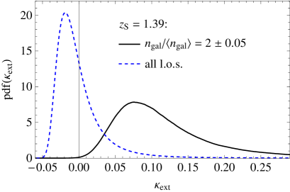
Figure 4.— Probability distribution for the external convergence $\kappa_{\mathrm{ext}}$ obtained from combining results of galaxy number counts around B1608$+$656 with results from ray-tracing through the Millennium Simulation. Compared are the distribution along lines of sight with a relative galaxy number density $n_{\mathrm{gal}}/\langle n_{\mathrm{gal}}\rangle=2.00\pm 0.05$ (solid line) to the distribution along all lines of sight (dotted line).

We can use this measurement of galaxy number density in the B1608$+$656 field to generate a more informative prior PDF for $\kappa_{\rm ext}$. As for the MS prior in the previous section, we use the ray-tracing through the MS together with the semi-analytic galaxy model of De Lucia & Blaizot (2007) to quantify the expected external convergence $\kappa_{\rm ext}$ for lines of sight with a given relative overdensity $n_{\mathrm{gal}}/\langle n_{\mathrm{gal}}\rangle$. Dividing out the absolute number of galaxies in the field accounts for differences due to the particular set of cosmological parameters used by the Millennium Simulation and inaccuracies in the galaxy model: We assume that differences in the relative overdensity between the MS cosmology and the true one are small.

We generate 32 simulated fields of $4\times 4\,\mathrm{deg}^{2}$ on the sky containing the positions and apparent magnitudes of the model galaxies at redshifts $0<z<5.2$ together with maps of the convergence $\kappa$ to source redshift $z_{\rm s}=1.39$. The galaxy positions and magnitudes in the simulated fields are converted into maps of the galaxy density $n_{\mathrm{gal}}$. We then select all lines of sight with relative overdensity $1.95\leq n_{\mathrm{gal}}/\langle n_{\mathrm{gal}}\rangle<2.05$ and compute the distribution of the convergence along these lines of sight. The resulting convergence distribution (shown in Figure 4) is then used as prior distribution for the external convergence $\kappa_{\mathrm{ext}}$, which we denote as the “OBS” (observations and MS) prior.

The convergence computed in this way is not strictly speaking external convergence, since (i) we do not subtract any contribution from any primary strong lens, (ii) we take all lines of sight and not just those to strong lenses. We are instead building on one of the results of the previous section and assume that the distribution of external convergences is very similar to the distribution of convergences along random lines of sight.

Where this approach becomes inappropriate is where a ray passes close to a galaxy center, and is hence associated with a very large convergence. Assuming such a line of sight as foreground/background for a strong lens galaxy essentially creates a lens system with two or more strong deflectors. These sightlines correspond to compound lenses such as SDSS J0946+1006 (Gavazzi et al., 2008), but not to B1608$+$656. However, the tail of high convergence values does not pose a problem here: as we will see in Section 8.1 below, the high external convergence is rejected by the dynamics modeling. We expect the mean and width of the PDF in Figure 4 to represent well the possible values of $\kappa_{\rm ext}$ for a field that is over-dense in galaxy number by a factor of two.

Our OBS $\kappa_{\rm ext}$ distribution agrees with earlier estimates from Fassnacht et al. (2006a), who identified and modeled the 4 groups along the line of sight to B1608$+$656 using various mass assignment recipes. In both approaches, we and Fassnacht et al. (2006a) are concerned primarily with extracting information on the external convergence and not the external shear. If we were to estimate the external convergence by assigning masses and redshifts to all objects in the B1608$+$656 field, and then ray tracing through the resulting model mass distribution, the external shear as required in the strong lens modeling would serve as an important calibrator for the external convergence. Such a procedure is beyond the scope of this paper, and we defer it to a future publication (Blandford et al., in preparation). However, we do find (by computing the distribution of external shears in MS fields with different external convergences) that the magnitude of the external shear required by the strong lens modeling ($\gamma_{\rm ext}\simeq 0.075)$ is consistent with the external shear amplitude predicted in the OBS scenario for the B1608$+$656 field.

6.3. The influence on lens modeling.

As already remarked, the description of ray propagation in an inhomogeneous cosmology is quite subtle. The matter (dark plus baryonic) density is partitioned between virialized structures (galaxies, groups and clusters) and a depleted background medium. Any structures sufficiently close to the line of sight will imprint convergence and shear onto a ray congruence. Meanwhile the background medium will contribute less Ricci focusing than would be present in a homogeneous, flat universe and will diminish the net convergence.

As the foregoing discussion makes clear, the line of sight to B1608$+$656 is unusual and we know quite a lot about the photometry and redshifts of the intervening galaxies. It is therefore possible, in principle, to make a refined estimate of the external convergence and shear and to compare the former with the simulations discussed above and the latter with the shear inferred in the lens model described in Paper I. In this way, the shear, again in principle, can be used to calibrate $\kappa_{\rm ext}$.

There is a second complication that must be addressed. Matter inhomogeneities in front of G1 and G2 distort the image of the primary lens as well as the multiple images of the source. Inhomogeneities behind the lens contribute further distortion in the images of the source. In a more accurate approach, these effects should be taken into account explicitly in the construction of the lens model, while here we are subsuming them in a single correction factor $\kappa_{\rm ext}$. The way that the resulting corrections affect the inference of a value for $H_{0}$ turns out to be quite complex. However, it appears that in the particular case of B1608$+$656, the error that is incurred does not contribute significantly to our quoted errors.

These matters will be discussed in a forthcoming publication.

7. Priors for model parameters ${\xi}$

A key goal of this work is to quantify the impact of the most serious systematic errors associated with using time-delay lenses for cosmography. Our approach is to characterize these errors as nuisance parameters, and then investigate the effects of various choices of prior PDF on the inference of cosmological parameters. To this end, we use either well motivated priors based on the results of Section 4, Section 6 and other independent studies, or, for contrast, uniform (maximally ignorant) prior PDFs. We now describe our choices for each parameter in turn.

• $P(\mbox{\boldmath{${\pi}$}})$. We consider a set of four cosmological parameters, $\mbox{\boldmath{${\pi}$}}=\{H_{0},\Omega_{\rm m},\Omega_{\rm\Lambda},w\}$. We then assign the following four different joint prior PDFs:

  K03: uniform prior on $H_{0}$ between $0$ and $150\ \rm{\,km\,s^{-1}\,Mpc^{-1}}$, $\Omega_{\rm m}=0.3$, $\Omega_{\rm\Lambda}=0.7$, and $w=-1$. This is the cosmology that was assumed in Koopmans et al. (2003) (the most recent $H_{0}$ measurement from B1608$+$656 before this work), and is the cosmology that is typically assumed in the literature for measuring $H_{0}$ from time-delay lenses. This form of prior allows us to compare our $H_{0}$ to earlier work.

  UNIFORM priors on all four cosmological parameters, with either the $w=-1$ or the flatness ($\Omega_{\rm m}=1-\Omega_{\rm\Lambda}$) constraint imposed. These priors allow us to quantify the information in the B1608$+$656 data set as conservatively as possible.

  WMAP5: WMAP 5 year data set posterior PDF for $\{H_{0},\Omega_{\rm m},\Omega_{\rm\Lambda},w\}$, assuming either $w=-1$ or a flat geometry. This allows us to constrain either flatness or $w$ by combining B1608$+$656 with WMAP.

  WBS: Joint posterior PDF for $\{H_{0},\Omega_{\rm\Lambda},w\}$ with a flat geometry, given the WMAP5 data in combination with compendia of BAO and supernovae (SN) data sets. This allows us to quantify the gain in precision made when incorporating B1608$+$656 into the current global analysis.

  The last two priors are defined by the Markov chains provided by the WMAP team based on the analysis performed by Dunkley et al. (2009) and Komatsu et al. (2009). The BAO data incorporated were taken from Percival et al. (2007); the SN sample used is the “union” sample of Kowalski et al. (2008). While the BAO and SN data sets are continually improving (e.g. Hicken et al., 2009), this particular well-defined snapshot is sufficient for us to explore the relative information content of our data set compared with other, well-known cosmological data sets. We also note that the publication of Markov chain representations of posterior PDFs makes further joint analyses like the one we present here very straightforward indeed.

• $P(\gamma^{\prime})$. We consider three different prior PDFs for the density profile slope. In the first two priors, we ignore the B1608$+$656 ACS data (i.e., dropping $P(\mbox{\boldmath{${d}$}}|\gamma^{\prime},\mbox{\boldmath{${\eta}$}},\mbox{\boldmath{${M}$}}_{\rm D}=\mbox{\boldmath{${M}$}}_{5})$ in Equation (30)); these first two are controls, to allow the assessment of the amount of information contained in the ACS data.

  Uniform: a maximally ignorant prior PDF, defined in the range $1.5\leq\gamma^{\prime}\leq 2.5$.

  SLACS: This is a Gaussian prior based on the result from the SLACS project: $\gamma^{\prime}=2.08\pm 0.2$ (Koopmans et al., 2009). This was derived from a sample of low-redshift massive elliptical lenses, studied with combined strong lens and stellar dynamics modeling. We note that this was obtained without considering the presence of any external convergence $\kappa_{\rm ext}$. However, Treu et al. (2009) find that the environmental effects in the SLACS lenses are smaller than their measurement errors and are typically undetected. Since SLACS lenses do not require an external shear in the modeling, typical $\kappa_{\rm ext}$ values for these lenses are expected to be small. Only in a few extreme cases does the $\kappa_{\rm ext}$ reach values of order $0.05$–$0.10$. Therefore, we take directly the prior on the slope from SLACS lenses without corrections for $\kappa_{\rm ext}$.

  ACS: This prior is the PDF $P(\gamma^{\prime}|\mbox{\boldmath{${d}$}},\mbox{\boldmath{${M}$}}_{\rm D}=\mbox{\boldmath{${M}$}}_{5})$ obtained from the analysis of the ACS image of B1608$+$656 in Section 4.2. This is the most informative of the three priors on $\gamma^{\prime}$, as it is determined directly from the B1608+656 data, independent of external priors from samples of galaxies (e.g. SLACS).

• $P(\mbox{\boldmath{${\eta}$}})$. As described in Section 4.2, we use the radio observations and the NICMOS F160W images of B1608$+$656 to constrain the smooth lens model parameters ${\eta}$ for a given slope $\gamma^{\prime}$. The posterior PDF from this analysis forms the prior PDF for the current work.

• $P(\kappa_{\rm ext})$. We consider three forms of prior for the external convergence:

  Uniform between $-0.25$ and $+0.25$: again, such a maximally ignorant prior, again to provide contrast.

  MS: from the strong lenses in the MS, discussed in Section 6.1.

  OBS: from the galaxy number counts in the field of B1608$+$656 and the MS, discussed in Section 6.2.

• $P(r_{\rm ani})$. For the lens galaxy stellar orbit radial anisotropy parameter $r_{\rm ani}$, we simply assign a uniform prior between $0.5r_{\rm eff}$ and $5r_{\rm eff}$, where $r_{\rm eff}$ is the effective radius that is determined from the photometry to be $0.58^{\prime\prime}\pm 0.06^{\prime\prime}$ (Koopmans et al., 2003) for the velocity dispersion measurement. The uncertainty in $r_{\rm eff}$ has negligible impact on the model velocity dispersion. The inner cutoff of $r_{\rm ani}$ is motivated by observations (e.g., Kronawitter et al., 2000) and radial instability arguments (e.g., Merritt & Aguilar, 1985; Stiavelli & Sparke, 1991), while the outer cutoff is for computational simplicity (the model velocity dispersion changes by a negligible amount between $r_{\rm ani}=5r_{\rm eff}$ and $r_{\rm ani}\rightarrow\infty$). These boundaries are consistent with those in Gebhardt et al. (2003).

These priors are summarized in Table 3.

8. Inference of $H_{0}$ and dark energy parameters from B1608$+$656

In this section we present the results of the analysis outlined in Section 3, putting together all the likelihood functions and prior PDFs described in Sections 4 to 7. We obtain $P(\mbox{\boldmath{${\pi}$}}|\mbox{\boldmath{${\Delta t}$}},\mbox{\boldmath{${d}$}},\sigma)$ by importance sampling, using the two likelihoods in Equation (33) as the weights for the various priors on $\gamma^{\prime}$, $\kappa_{\rm ext}$, $r_{\rm ani}$, and ${\pi}$ listed in Table 3 (see Appendix A.2 for details). By using the likelihood functions of our B1608$+$656 data sets, we are incorporating the uncertainties associated with these measurements. We expect and indeed find that the data are relatively insensitive to $r_{\rm ani}$ and do not constrain it. Focusing first on the systematic errors now quantified as the nuisance parameters $\gamma^{\prime}$ and $\kappa_{\rm ext}$, we gradually increase the complexity of the cosmological model to probe the full space of parameters.

For each possible combination of the priors on the parameters in Table 3, we generate 96000 samples of $\gamma^{\prime}$, $\kappa_{\rm ext}$, $r_{\rm ani}$, and ${\pi}$ to characterize the prior probability distribution. We also have two types of stellar distribution functions, Hernquist and Jaffe, for modeling the stellar velocity dispersion; we find that the two different types of stellar distribution function produce nearly identical PDFs for the cosmological parameters. Since the priors on the parameters play a greater role than does the choice of stellar dynamics model, we focus only on the Hernquist stellar distribution function for the remainder of the section.

Table 3 Priors on the parameters

$P(\gamma^{\prime})$	uniform ($1.5\leq\gamma^{\prime}\leq 2.5$)	SLACS ($\gamma^{\prime}=2.08\pm 0.2$)	ACS ($\gamma^{\prime}=2.08\pm 0.03$)
$P(\kappa_{\rm ext})$	uniform ($-0.25\leq\kappa_{\rm ext}\leq 0.25$)	MS (Millennium Simulations; Figure 3)	OBS (Observations and MS; Figure 4)
$P(r_{\rm ani})$	uniform ($0.5r_{\rm eff}\leq r_{\rm ani}\leq 5r_{\rm eff}$)
$P(\mbox{\boldmath{${\pi}$}})$	K03 ($\Omega_{\rm m}=0.3$, $\Omega_{\rm\Lambda}=0.7$, $w=-1$,	UNIFORMopen ($w=-1$,	UNIFORMw ($\Omega_{\rm\Lambda}=1-\Omega_{\rm m}$ uniform $\in[0,1]$,
	uniform $H_{0}\in[0,150]\,\rm{\,km\,s^{-1}\,Mpc^{-1}}$)	$\Omega_{\rm m}$ and $\Omega_{\rm\Lambda}$ uniform $\in[0,1]$,	uniform $w\in[-2.5,0.5]$,
		uniform $H_{0}\in[0,150]\,\rm{\,km\,s^{-1}\,Mpc^{-1}}$)	uniform $H_{0}\in[0,150]\,\rm{\,km\,s^{-1}\,Mpc^{-1}}$)
	WMAPopen	WMAPw (WMAP5 with	WBSw (WMAP5 + BAO + SN with
	(WMAP5 with $w=-1$)	flatness and time-independent $w$)	flatness and time-independent $w$)

Notes — The K03 entry for $P(\mbox{\boldmath{${\pi}$}})$ is the same prior as in Koopmans et al. (2003). This is also the most common cosmology prior assumed in previous studies of time-delay lenses.

8.1. Exploring the degeneracies among $H_{0}$, $\gamma^{\prime}$ and $\kappa_{\rm ext}$

To investigate the impact of our limited knowledge of the lens density profile slope $\gamma^{\prime}$ and external convergence $\kappa_{\rm ext}$, we first fix the cosmological parameters $\Omega_{\rm m}$, $\Omega_{\rm\Lambda}$ and $w$ according to the K03 prior. This allows us a simplified view of the problem, and also a comparison with previous work that used this rather restrictive prior.

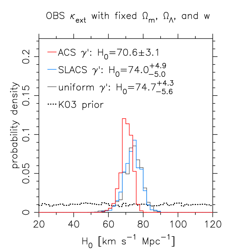
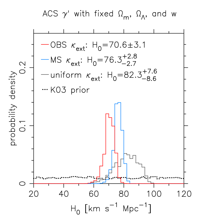
Figure 5.— Left: the marginalized posterior PDF for $H_{0}$ assuming K03 cosmology and OBS $\kappa_{\rm ext}$ priors. Right: the marginalized posterior PDF for $H_{0}$ assuming K03 cosmology and ACS $\gamma^{\prime}$ priors. The prior uncertainty in external convergence determines the precision of the inferred Hubble constant.

We first assign the OBS prior for $\kappa_{\rm ext}$, and look at the effect of the various choices of density profile slope priors. The left-hand panel in Figure 5 shows the marginalized posterior PDF for $H_{0}$ for the three different priors for $\gamma^{\prime}$ given in Table 3. From this graph, we see that the SLACS prior gives a similar estimate of $H_{0}$ as the uniform prior with a negligible increase in precision. The ACS prior lowers $H_{0}$ relative to that of the SLACS and uniform priors, and improves the precision in $H_{0}$ to $4.4\%$. Overall, the impact of the prior on $\gamma^{\prime}$ is relatively low in the sense that, even with a uniform prior on $\gamma^{\prime}$, $H_{0}$ is still constrained to $7\%$ (taking $H_{0}=70.6$ as our reference value). For the remainder of this paper, we assign the ACS prior.

As expected, the prior for $\kappa_{\rm ext}$ has a greater effect, shown in the right-hand panel of Figure 5. Taking the maximally informative OBS prior as our default, we see that relaxing this to the MS prior causes an increase in inferred $H_{0}$ value of some $6\rm{\,km\,s^{-1}\,Mpc^{-1}}$, and relaxing further to a uniform prior increases it by $12\rm{\,km\,s^{-1}\,Mpc^{-1}}$. The precision in $H_{0}$ also drops by more than a factor of two from the OBS prior to the uniform prior. Our knowledge of $\kappa_{\rm ext}$ is therefore limiting the inference of $H_{0}$.

We note that the stellar dynamics contain a significant amount of information on $H_{0}$. The stellar dynamics effectively constrain $\kappa_{\rm ext}$ and $\gamma^{\prime}$ to an approximately linear relation, where an increase in $\kappa_{\rm ext}$ requires a steepening of the slope in order to keep the predicted velocity dispersion the same. Therefore, for a fixed range of $\gamma^{\prime}$ values, the modeling of the stellar dynamics would only permit a corresponding range of $\kappa_{\rm ext}$ values. Specifically, without dynamics as constraints, we find $H_{0}=68.1^{+3.7}_{-6.4}\rm{\,km\,s^{-1}\,Mpc^{-1}}$ for the ACS and OBS priors. The lower bound on $H_{0}$ is somewhat weakened by the high tail of the OBS $\kappa_{\rm ext}$ distribution. On the other hand, this high tail is rejected by the use of the dynamics data. Therefore, our tight constraint on $H_{0}$ results from the combination of all available data sets – each data set constrains different parts of the parameter space such that the joint distribution is tighter than the individual ones.

To summarize, using all available information on B1608$+$656 and the ACS and OBS priors gives $H_{0}=70.6\pm{3.1}\rm{\,km\,s^{-1}\,Mpc^{-1}}$, a precision of $4.4\%$. We interpret Figure 5 as evidence that we are approaching saturation in the information we have on the lens model for B1608$+$656: the mass model is now so well constrained that the inference of cosmological parameters from this system is limited by our knowledge of the lens environment. We now explore this joint inference in more detail, first putting it in some historical context.

8.2. Comparison with other lensing $H_{0}$ results

What improvement in the measurement of $H_{0}$ do we gain from our new observations of B1608$+$656? The most recent measurement before this work by Koopmans et al. (2003) was $H_{0}=75^{+7}_{-6}\rm{\,km\,s^{-1}\,Mpc^{-1}}$. This result was based on a joint lensing and dynamics modeling using the radio data, shape of the Einstein ring from the NICMOS images and the earlier less precise velocity dispersion measurement. Our improved analysis using the deep ACS images and the newly measured velocity dispersion reduce the uncertainty by more than a factor of two, even with the inclusion of the systematic error due to the external convergence that was previously neglected. We attribute our lower $H_{0}$ value to our incorporation of the realistically-skewed OBS $\kappa_{\rm ext}$.

Let us now compare our $H_{0}$ measurement based on the K03 cosmology to several recent measurements (within the past five years) from other time-delay lenses. Most analyses assumed $\Omega_{\rm m}=0.3$ and $\Omega_{\rm\Lambda}=0.7$ — we point out explicitly the few that did not. In B0218+357, Wucknitz et al. (2004) measured $H_{0}=78\pm 6\,\rm{\,km\,s^{-1}\,Mpc^{-1}}$ ($2\sigma$) by modeling this two-image lens system with isothermal elliptical potentials (and effectively measuring $\gamma^{\prime}$, see Section 4.2.3) but neglecting external convergence. York et al. (2005) refined this using the centroid position of the spiral lens galaxy based on HST/ACS observations as a constraint; depending on the spiral arm masking, they found $H_{0}=70\pm 5\,\rm{\,km\,s^{-1}\,Mpc^{-1}}$ (unmasked) and $H_{0}=61\pm 7\,\rm{\,km\,s^{-1}\,Mpc^{-1}}$ (masked) (both with $2\sigma$ errors). In the two-image FBQ 0951+2635, Jakobsson et al. (2005) obtained $H_{0}=60^{+9}_{-7}$ (random, $1\sigma$) $\pm 2$ (systematic) $\rm{\,km\,s^{-1}\,Mpc^{-1}}$ for a singular isothermal ellipsoid model and $H_{0}=63^{+9}_{-7}$ (random, $1\sigma$) $\pm 1$ (systematic) $\rm{\,km\,s^{-1}\,Mpc^{-1}}$ for a constant mass-to-light ratio model, again ignoring external convergence. In the two-image quasar system SDSS J1650+4251, Vuissoz et al. (2007) found $H_{0}=51.7^{+4.0}_{-3.0}\rm{\,km\,s^{-1}\,Mpc^{-1}}$ assuming a singular isothermal sphere and constant external shear for the lens model. More general lens models considered by these authors (e.g. including lens ellipticity, or using a de Vaucouleurs density profile) were found to be underconstrained. In the two-image quasar system SDSS J1206+4332, Paraficz et al. (2009) found $H_{0}=73^{+3}_{-4}\rm{\,km\,s^{-1}\,Mpc^{-1}}$ using singular isothermal ellipsoids or spheres to describe the three lens galaxies, where photometry was used to place additional constraints on the lens parameters. Recently, Fadely et al. (2009) modeled the gravitational lens Q0957+561 using four different dark matter density profiles, each with a stellar component. The lens is embedded in a cluster, and the authors constrained the corresponding mass sheet using the results of a weak lensing analysis by Nakajima et al. (2009). Assuming a flat universe with $\Omega_{\rm m}=0.274$ and cosmological constant $\Omega_{\rm\Lambda}=0.726$, they found $H_{0}=85^{+14}_{-13}\rm{\,km\,s^{-1}\,Mpc^{-1}}$, where the principle uncertainties were due to the weakly constrained stellar mass-to-light ratio (a manifestation of the radial profile degeneracy in the lens model). Imposing constraints from stellar population synthesis models led to $H_{0}=79.3^{+6.7}_{-8.5}\rm{\,km\,s^{-1}\,Mpc^{-1}}$.

In a nutshell, most of the recent $H_{0}$ measurements from individual systems assumed isothermal profiles, and neglected the effects of both $\gamma^{\prime}$ and $\kappa_{\rm ext}$: we interpret the significant variation between the $H_{0}$ estimates in the recent literature as being due to these model limitations. In contrast, our B1608$+$656 analysis explicitly incorporates the uncertainties due to our lack of knowledge of both $\gamma^{\prime}$ and $\kappa_{\rm ext}$. In fact, a spread of $\sim 0.2$ in $\gamma^{\prime}$ around $2.0$ would give a spread of $\sim 40\%$ in $H_{0}$ for the cases where isothermal lenses are assumed (Wucknitz, 2002). These in turn are set by a lack of information on the systems, either because only two images are formed, or the extended source galaxy is not observed.

Other groups have looked to improve the constraints on $H_{0}$ by combining several lenses together in a joint analysis. Using a sample of 10 time-delay lenses, Saha et al. (2006) measured $H_{0}=72^{+8}_{-11}\rm{\,km\,s^{-1}\,Mpc^{-1}}$ by modeling the lens’ convergence distributions on a grid and using the point image positions of the lenses as constraints (the PixeLens method). Coles (2008) improved on the method and obtained $H_{0}=71^{+6}_{-8}\rm{\,km\,s^{-1}\,Mpc^{-1}}$ while addressing more clearly their prior assumptions. Oguri (2007) used a sample of 16 time-delay lenses to constrain $H_{0}=68\pm 6{\rm(stat.)}\pm 8{\rm(syst.)}\rm{\,km\,s^{-1}\,Mpc^{-1}}$ (for $\Omega_{\rm m}=0.24$ and $\Omega_{\rm\Lambda}=0.76$; see footnote 9) by employing a statistical approach based on the image configurations. By simultaneously modeling SDSS J1206+4332 with four other systems using PixeLens, Paraficz et al. (2009) derive $H_{0}=61.5^{+8}_{-4}\rm{\,km\,s^{-1}\,Mpc^{-1}}$. The larger quoted error bars on these ensemble estimates are perhaps a reflection of the paucity of information available for each lens, as discussed above. All four analyses effectively assume that the ensemble external convergence distribution has zero mean, which may not be accurate: for example, Oguri (2007) constructed a sample for which external convergence could be neglected, and then incorporated this into the systematic error budget. Furthermore, Oguri (2007) imposed a Gaussian prior on the slope of $\gamma^{\prime}=2.00\pm 0.15$, and the PixeLens method’s priors on $\kappa$ may well implicitly impose constraints on $\gamma$ that are similar to the prior in Oguri (2007); these priors on the slope may not be appropriate for individual systems in the ensembles.

In contrast, our measurement of $\gamma^{\prime}$ from the ACS data means that our results are independent of external priors on $\gamma^{\prime}$. In fact, our detailed study of the single well-observed lens B1608$+$656, even incorporating the effects of $\kappa_{\rm ext}$, constrains $H_{0}$ better than the studies using ensembles of lenses. Our claim is that our analysis of the systematic effects in B1608$+$656 — explicitly including density profile slope and external convergence as nuisance parameters — is one of the most extensive on a single lens, and is rewarded with one of the most accurate measurements of $H_{0}$ from time-delay lenses.

8.3. Relaxing the K03 prior

As we described in Section 2, strong lens time delays enable a measurement of a cosmological distance-like quantity, $D_{\rm\Delta t}\equiv(1+z_{\rm d})D_{\rm d}D_{\rm s}/D_{\rm ds}$. While there is some slight further dependence on cosmology in the stellar dynamics modeling, we expect this particular distance combination to be well constrained by the system. To illustrate this, we plot in Figure 6 the PDF for $D_{\rm\Delta t}$ with and without the constraints from B1608$+$656, for various choices of the cosmological parameter prior PDF. Specifically, we show the effect of relaxing the prior on $\Omega_{\rm m}$, $\Omega_{\rm\Lambda}$ and $w$ from the K03 delta function to the two types of uniform distributions detailed in Table 3: “UNIFORMopen” and “UNIFORMw”. We see that all of these distributions predict the same uninformative prior for $D_{\rm\Delta t}$, and that the B1608$+$656 posterior PDFs are correspondingly similar. With the OBS and ACS priors for $\kappa_{\rm ext}$ and $\gamma^{\prime}$, we estimate $D_{\rm\Delta t}\simeq(5.16^{+0.29}_{-0.24})\times 10^{3}\,{\mathrm{Mpc}}$, a precision of $\sim 5\%$. The difference between the $D_{\rm\Delta t}$ estimates among the three priors shown is $\lesssim 2\%$.

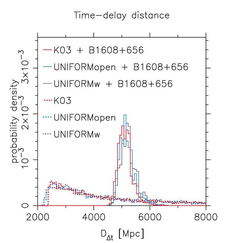
Figure 6.— PDFs for $D_{\rm\Delta t}$, showing the B1608$+$656 posterior constraints on $D_{\rm\Delta t}$ (solid) given assorted uniform priors for the cosmological parameters (dotted, labeled). See the text for a full description of these various priors. In this figure we assign the ACS and OBS priors for $\gamma^{\prime}$ and $\kappa_{\rm ext}$. B1608$+$656 provides tight constraints on $D_{\rm\Delta t}$, which translates into information about $\Omega_{\rm m}$, $\Omega_{\rm\Lambda}$ and $w$ as well as $H_{0}$.

Figure 6 suggests that a shifted log normal approximation (to take into account the skewness) for the product of the B1608$+$656 likelihood function, marginalized over the OBS and ACS priors, is an appropriate compression of our results. We find that

$$P(D_{\rm\Delta t}|H_{0},\Omega_{\rm m},\Omega_{\rm\Lambda},w)\simeq$$ (35)

$$\frac{1}{\sqrt{2\pi}(x-\lambda_{\rm D})\sigma_{\rm D}}\exp{\left[-\frac{(\log(x-\lambda_{\rm D})-\mu_{\rm D})^{2}}{2\sigma_{\rm D}^{2}}\right]},$$

where $x=D_{\rm\Delta t}/(1\,{\rm Mpc})$, $\lambda_{\rm D}=4000.$, $\mu_{\rm D}=7.053$ and $\sigma_{\rm D}=0.2282$, accurately reproduces the cosmological parameter inferences: for example, Hubble’s constant is recovered to $<0.7\%$ and its $16^{\rm th}$ and $84^{\rm th}$ percentiles (68% CL) are recovered to $<1.1\%$ for the WMAP cosmologies we considered.

8.4. Constraints on $\Omega_{\rm m}$ and $\Omega_{\rm\Lambda}$

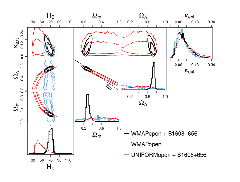
Figure 7.— The B1608$+$656 marginalized posterior PDF for $H_{0}$, $\Omega_{\rm m}$, $\Omega_{\rm\Lambda}$ and $\kappa_{\rm ext}$ in a $w=-1$ cosmological model and assuming ACS $\gamma^{\prime}$ and OBS $\kappa_{\rm ext}$ priors; contours are 68% and 95% confidence levels. The three sets of colored contours correspond to three different prior/data set combinations. Blue: B1608$+$656 constraints, given the UNIFORMopen prior; red: the prior provided by the WMAP 5 year data set alone; black: the joint constraints from combining WMAP and B1608$+$656. The blue contours in the $\Omega_{\rm m}$ and $\Omega_{\rm\Lambda}$ columns are omitted since they would show almost no constraints, as indicated by the diagonal panels.

Based on the construction of $D_{\rm\Delta t}$, we expect strong lens time delays to be more sensitive to $H_{0}$ than the other three cosmological parameters. This is shown in Figure 7, where we consider $w=-1$ uniform cosmological prior “UNIFORMopen” and plot the marginalized B1608$+$656 posterior PDF to show the influence of the lensing data (blue lines). While there is a slight dependence on $\Omega_{\rm\Lambda}$, we see that the B1608$+$656 data do indeed primarily constrain $H_{0}$. In contrast, we plot the posterior PDF from the analysis of the 5 year WMAP data set (red lines, Dunkley et al., 2009). With no constraint on the curvature of space, the CMB data provides only a weak prior on $H_{0}$, which is highly degenerate with $\Omega_{\rm m}$ and $\Omega_{\rm\Lambda}$. Importance sampling the WMAP MCMC chains with the B1608$+$656 likelihood, we obtain the joint posterior PDF, plotted in black.

Strong lens time delays are an example of a kinematic cosmological probe, i.e., one that is sensitive to the geometry and expansion rate of the Universe, but not to dynamical assumptions about the the growth of structure in the Universe. In Table 4, we compare the B1608$+$656 data set to a number of other kinematic probes from the literature. The WMAP data constrain the angular diameter distance to the last scattering surface; these other data sets effectively provide a second distance estimate that breaks the degeneracy between $H_{0}$ and the curvature of space. In the B1608$+$656 case, we constrain $\Omega_{\rm k}$ to be $-0.005_{-0.026}^{+0.014}$ (95% CL). We can see that in terms of constraining the curvature parameter, B1608$+$656 is more informative than the HST Key Project $H_{0}$ measurement, and is comparable to the current SNe Ia data set.

Table 4 Curvature parameter constraints from WMAP5 combined with various data sets assuming $w=-1$ (95% CL).

WMAP5a,b	$-0.285<\Omega_{\rm k}<0.010$	$15\%$
WMAP5 + HST  KPb,c	$-0.052<\Omega_{\rm k}<0.013$	$3.3\%$
WMAP5 + SNb,d	$-0.032<\Omega_{\rm k}<0.008$	$2.0\%$
WMAP5 + BAOb,e	$-0.017<\Omega_{\rm k}<0.007$	$1.2\%$
WMAP5 + B1608	$\mathbf{-0.031<\Omega_{\rm k}<0.009}$	$\mathbf{2.0\%}$

The third column gives the “precision,” quantified as half the 95% confidence interval in $(1.0-\Omega_{\rm k})$, as a percentage.   ^a http://lambda.gsfc.nasa.gov    ^b Komatsu et al. (2009).   ^c Freedman et al. (2001).   ^d Based on the “union” SN samples compiled by Kowalski et al. (2008).   ^e Percival et al. (2007).  

Figure 7 also shows the primary nuisance parameter, $\kappa_{\rm ext}$. When B1608$+$656 and the WMAP data are combined, the PDF for $\kappa_{\rm ext}$ shifts and tightens very slightly, as we expect from the discussion in Section 8.1. If we relax the OBS prior on $\kappa_{\rm ext}$ to uniform, then we obtain $-0.032<\Omega_{\rm k}<0.021$ (95% CL), which is still tighter than the HST KP constraints.

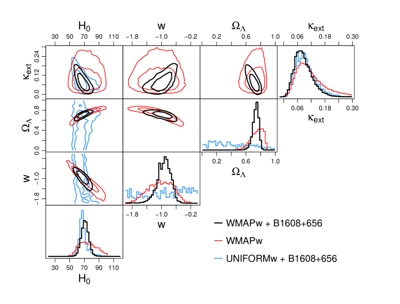
Figure 8.— The B1608$+$656 marginalized posterior PDF for $H_{0}$, $\Omega_{\rm\Lambda}$, $w$ and $\kappa_{\rm ext}$ in a flat cosmological model, again assuming ACS $\gamma^{\prime}$ and OBS $\kappa_{\rm ext}$ priors; contours are 68% and 95% confidence levels. The three sets of colored contours correspond to three different prior/data set combinations. Blue: B1608$+$656 constraints, given the UNIFORMw prior; red: the prior provided by the WMAP 5 year data set alone; black: the joint constraints from combining WMAP and B1608$+$656. The blue contours in the $\Omega_{\rm m}$ and $\Omega_{\rm\Lambda}$ columns are omitted since they would show almost no constraints, as indicated by the diagonal panels.

8.5. Constraints on dark energy

As noted by many authors (e.g. Hu, 2005; Komatsu et al., 2009; Riess et al., 2009), the degeneracy-breaking shown in the previous subsection can be recast as a mechanism for constraining the equation of state of dark energy, $w$. If we assert a precisely flat geometry for the Universe, as motivated by the inflationary scenario, we can spend our available information on constraining $w$ instead. Figure 8 shows the marginalized posterior PDF for the cosmological parameter $H_{0}$, $\Omega_{\rm\Lambda}=1-\Omega_{\rm m}$ and $w$, along with the nuisance parameter $\kappa_{\rm ext}$, again comparing the B1608$+$656 constraints with uniform and WMAP priors, and the WMAP constraints alone. With the WMAP data alone, $w$ is strongly degenerate with $H_{0}$ and $\Omega_{\rm\Lambda}$. Including B1608$+$656, which mainly provides constraints on $H_{0}$, the $H_{0}$-$w$-$\Omega_{\rm\Lambda}$ degeneracy is partly broken. The resulting marginalized distribution gives $w=-0.94^{+0.17}_{-0.19}$, consistent with a cosmological constant. The corresponding value of Hubble’s constant is $H_{0}=69.7^{+4.9}_{-5.0}\rm{\,km\,s^{-1}\,Mpc^{-1}}$.

We summarize our inferences of $H_{0}$ and $w$ in this variable-$w$ model in Table 5, comparing to a similar set of alternative kinematic probes referred to in the previous section. We see that, combining with the WMAP 5 year data set and marginalizing over all other parameters, the B1608$+$656 data set provides a measurement of Hubble’s constant with an uncertainty of 6.9%, with the equation of state parameter simultaneously constrained to 18%. This level of precision is better than that available from the HST  KP and is competitive with the current BAO measurements.

Our results are consistent with the results from all the other probes listed. This is not a trivial statement: combining each data set with the WMAP 5 year prior allows us not only to quantify the relative constraining power of each one, it also retains the possibility of detecting inconsistencies between data sets. As it is, it appears that all the kinematic probes listed are in agreement within their quoted uncertainties. Some tension might be present if the supernovae and B1608$+$656 were considered separately from a combination of local HST  $H_{0}$ measurements and BAO constraints, but we have no compelling reason to make such a division. As the statistical errors associated with each probe are decreased, other inconsistencies may arise: we might expect there to always be a need for careful pairwise data set combinations.

Finally then, we incorporate B1608$+$656 into a global analysis of cosmological data sets. As an example, we importance sample from the WBSw prior PDF; this is the joint posterior PDF from the joint analysis of WMAP5, BAO and SN data. This prior is already very tight, characterized by a median and 68% confidence limits of $H_{0}=70.3^{+1.6}_{-1.5}\rm{\,km\,s^{-1}\,Mpc^{-1}}$. When we include information from B1608$+$656 with the ACS $\gamma^{\prime}$ and OBS $\kappa_{\rm ext}$ priors, we obtain $H_{0}=70.4^{+1.5}_{-1.4}\rm{\,km\,s^{-1}\,Mpc^{-1}}$, a slight shift in centroid and 6% reduction in the confidence interval. This is good as it shows global consistency in the WMAP5, BAO, SN and B1608$+$656 data sets.

Table 5 Dark energy constraints from WMAP5 combined with various data sets, assuming flat geometry.

	$H_{0}/\rm{\,km\,s^{-1}\,Mpc^{-1}}$			$w$
WMAP5a,b	$74^{+15}_{-14}$	$20\%$		$-1.06^{+0.41}_{-0.42}$	$42\%$
WMAP5+HST  KPa,b,c	$72.1^{+7.4}_{-7.6}$	$10\%$		$-1.01^{+0.23}_{-0.22}$	$23\%$
WMAP5+SNa,b,d	$69.4^{+1.6}_{-1.7}$	$2.3\%$		$-0.977^{+0.065}_{-0.064}$	$6.5\%$
WMAP5+BAOa,b,e	$73.9^{+4.7}_{-4.8}$	$6.6\%$		$-1.15^{+0.21}_{-0.22}$	$22\%$
WMAP5+Riessf	$74.2\pm 3.6^{\rm g}$	$5.0\%$		$-1.12\pm 0.12$	$12\%$
WMAP5+B1608	$\mathbf{69.7^{+4.9}_{-5.0}}$	$\mathbf{6.9\%}$		$\mathbf{-0.94^{+0.17}_{-0.19}}$	$\mathbf{18\%}$

The “precisions” in the third and fifth columns are defined as half the 68% confidence interval, as a percentage of either 72 for $H_{0}$ or -1.0 for $w$.    ^a http://lambda.gsfc.nasa.gov    ^b Komatsu et al. (2009). The $H_{0}$ estimate was taken from the previously listed website.   ^c Freedman et al. (2001).   ^d Based on the “union” SN samples compiled by Kowalski et al. (2008).   ^e Percival et al. (2007).   ^f Riess et al. (2009).   ^g not marginalized over other cosmological parameters.

8.6. Future prospects

In this paper, we have studied a single strong gravitational lens, B1608$+$656, investigating in depth the various model parameter degeneracies and systematic effects. At present, B1608$+$656 remains the only strong lens system with (i) time delay measurements with errors of only a few percent, and (ii) extended source surface brightness distribution for accurate lens modeling; as we have shown, these two properties together enable the careful study and the resulting tight constraint on $H_{0}$.

Table 5 shows that even this one system provides competitive accuracy on $H_{0}$ and $w$ for a single kinematic probe, especially when we consider that all the other experiments involved averaging together many independent distance measurements. What should we expect from extending this study to many more lenses? As we showed in Section 8.1, if the data are good enough to constrain the density profile slope to a few percent, the accuracy of the cosmological parameter inference is limited, as it is in B1608$+$656, by our knowledge of the lens environment, $\kappa_{\rm ext}$.

However, we also outlined in Section 6 how using information from numerical simulations and the photometry in the field can be used to constrain this nuisance parameter and yield an unbiased estimate of $H_{0}$. Furthermore, as discussed in Section 8.1, stellar dynamics provides significant amount of information on $\kappa_{\rm ext}$ by limiting its permissible range of values. While we, and also Treu et al. (2009) and Fassnacht et al. (2009), discuss how the line-of-sight contributions to $\kappa_{\rm ext}$ should average to zero over many lens systems, lens galaxies — like all massive galaxies — tend to live in locally overdense environments, such that the local contribution to $\kappa_{\rm ext}$ would be non-zero. Careful studies of the lens environments (e.g. Momcheva et al. 2006; Fassnacht et al. 2006a; Blandford et al. in preparation) and of N-body simulations with gas physics to determine this local contribution to $\kappa_{\rm ext}$ will be crucial for obtaining $H_{0}$ from a large sample of lenses. If we are able to average together $N$ systems we should, in principle, be able to reduce our uncertainty by $\sqrt{N}$. In practice, the accuracy of the combination procedure will sooner be limited by the systematic uncertainty in the shape and centroid of the assumed $\kappa_{\rm ext}$ distribution: investigating the properties of this distribution is perhaps the most urgent topic for further work. Likewise, if the density profile slope cannot be constrained for each time-delay lens individually, the details of the prior PDF assigned for $\gamma^{\prime}$ will become important as the ensemble grows.

In the near future, cadenced surveys such as those planned with the Large Synoptic Survey Telescope (LSST) and being undertaken by the Panoramic Survey Telescope and Rapid Response System (Pan-STARRS) will discover large numbers of time-delay lenses, prompting us to consider performing analyses such as the one described here on hundreds of lens systems. In practice, obtaining data of the quality we have presented here for hundreds of suitable lenses will pose a significant observational challenge. Nevertheless, Dobke et al. (2009), Coe & Moustakas (2009) and Oguri & Marshall (in preparation) investigate constraints on cosmological parameters based on large samples of time-delay lenses. In particular, Coe & Moustakas (2009) suggest that, in terms of raw precision and in combination with a prior PDF from Planck, an LSST ensemble could reach sub-percent level precision in $H_{0}$, and constrain $w$ to 3% or better, provided that the systematic effects such as $\kappa_{\rm ext}$ are under control. Our work has already addressed some of these systematic effects, and will provide a basis for future analysis of large samples of time-delay lenses and lens environment studies.

9. Conclusions

We have studied the well-observed gravitational lens B1608$+$656 and used it to infer the values of cosmological parameters; we outlined and followed a Bayesian approach for combining three data sets: HST/ACS imaging, stellar velocity dispersion measurement, and the time delays between the multiple images. Diagnosing the principal systematic effects, we included two nuisance parameters ($\gamma^{\prime}$ and $\kappa_{\rm ext}$) into the data model to account for them, assigning well-motivated prior PDFs and marginalizing over them. We draw the following conclusions:

• We find that the HST/ACS images constrain the density profile slope parameter $\gamma^{\prime}=2.08\pm 0.03$, which we propagate through the cosmological parameter inference as a prior PDF. Relaxing this prior to a uniform distribution degrades the precision on $H_{0}$ from 4.4% to 7.0%; the SLACS intrinsic profile slope parameter distribution is not significantly more informative than the uniform prior.

• With the ACS prior for $\gamma^{\prime}$, we find that the inferred cosmological parameters are dominated by the the external convergence $\kappa_{\rm ext}$. Ray-tracing through the Millennium Simulation gives a PDF for $\kappa_{\rm ext}$ due to line-of-sight contributions that has zero mean and width $\sim 0.04$, while using the galaxy number counts in the B1608$+$656 field in conjunction with the MS gives $\kappa_{\rm ext}=0.10^{+0.08}_{-0.05}$.

Using our most informative priors on the two nuisance parameters, we arrive at the following cosmographic inferences:

• In the K03 cosmology ($\Omega_{\rm m}=0.3$, $\Omega_{\rm\Lambda}=0.7$, $w=-1$, and uniform $H_{0}$), we obtain from the B1608$+$656 data set $H_{0}=70.6\pm 3.1\rm{\,km\,s^{-1}\,Mpc^{-1}}$ (68% CL). The $4.4\%$ error includes both statistical and dominant systematic uncertainties, through the marginalization described above. This is a significant improvement to the earlier measurement of $H_{0}=75^{+7}_{-6}\rm{\,km\,s^{-1}\,Mpc^{-1}}$ by Koopmans et al. (2003).

• Time-delay lenses are sensitive primarily to $H_{0}$ but are weakly dependent on other cosmological parameters; the lensing measurement of $H_{0}$ is robust and useful for studying dark energy when combined with other cosmological probes. We find that for B1608$+$656 the cosmographic information can be summarized as a shifted log normal probability distribution for the time-delay distance $D_{\rm\Delta t}$ in units of Mpc, with the three parameters $\lambda_{\rm D}=4000.$, $\mu_{\rm D}=7.053$ and $\sigma_{\rm D}=0.2282$.

• In a $\Lambda$-CDM cosmology (with $w=-1$), the B1608$+$656 data set breaks the degeneracy between $\Omega_{\rm m}$ and $\Omega_{\rm\Lambda}$ in the WMAP 5 year data set, and constrains the curvature parameter to be zero to $2.0\%$ (95% CL), a level of precision similar to those afforded by the current Type Ia SNe sample.

• B1608$+$656 in combination with the WMAP 5 year data set, assuming flatness and allowing (a time-independent) $w$ to vary, gives $H_{0}=69.7^{+4.9}_{-5.0}\rm{\,km\,s^{-1}\,Mpc^{-1}}$ and $w=-0.94^{+0.17}_{-0.19}$ (68% CL).

  These are significant improvements to the WMAP5 only constraints of $H_{0}=74^{+15}_{-14}\,\rm{\,km\,s^{-1}\,Mpc^{-1}}$ and $w=-1.06^{+0.41}_{-0.42}$. B1608$+$656 is as competitive as the current BAO data in determining $w$ when combined with WMAP5.

Our detailed analysis of B1608$+$656 provides the framework for using large samples of time-delay lenses as cosmological probes in the near future. We anticipate the local contribution to $\kappa_{\rm ext}$, which would not average away with a large sample of lenses, being the dominant residual systematic error. Several lens environment studies to circumvent this are underway; with the effects from $\kappa_{\rm ext}$ accurately modeled, future samples of time-delay gravitational lenses should be a competitive cosmological probe.

Appendix A Probability Theory for Measuring Cosmological Parameters

In this appendix, we describe how we derive the expressions for the likelihoods of the time delay and the ACS data sets stated in Section 3.3. We also provide the details on the sampling techniques for calculating the posterior probability density of cosmological parameters.

A.1. Simplification of the likelihoods

For B1608$+$656, we can simplify the marginalization of the likelihoods $P(\mbox{\boldmath{${\Delta t}$}}|\mbox{\boldmath{${\xi}$}})$ and $P(\mbox{\boldmath{${d}$}}|\mbox{\boldmath{${\xi}$}})$ in Equation (24) based on the following facts, which are either from Paper I or shown in Section 4:

• from Paper I, the top $\mbox{\boldmath{${M}$}}_{\rm D}$ models led to equal evidence values $P(\mbox{\boldmath{${d}$}}|\gamma^{\prime},\mbox{\boldmath{${\eta}$}},\mbox{\boldmath{${\delta\psi}$}}_{\mathrm{MP}},\mbox{\boldmath{${M}$}}_{\rm D})$ (within the uncertainties).

• in Section 4, the likelihood function $P(\mbox{\boldmath{${\Delta t}$}}|\mbox{\boldmath{${\xi}$}})$ is approximately constant for these top $\mbox{\boldmath{${M}$}}_{\rm D}$ models for a given cosmology.

• in Section 4, for good data models $\mbox{\boldmath{${M}$}}_{\rm D}$ of B1608$+$656, the potential corrections ${\delta\psi}$ do not change significantly the predicted values of the Fermat potential, i.e., the simply-parametrized SPLE initial model provides an unbiased estimator for the Fermat potential.

• the likelihood $P(\sigma|\mbox{\boldmath{${\xi}$}})$ is also constant for the various $\mbox{\boldmath{${M}$}}_{\rm D}$ because the dynamics modeling is independent of the lensed image processing models $\mbox{\boldmath{${M}$}}_{\rm D}$.

• simulations suggest that the potential corrections ${\delta\psi}$ are sharply peaked about the most probable values $\mbox{\boldmath{${\delta\psi}$}}_{\mathrm{MP}}$.

With the above results, the Fermat potential can be more easily computed from the SPLE model: there is a strong correlation between the $\Delta\phi$ and $\gamma^{\prime}$, and we obtain the relation between $\Delta\phi$ and $\gamma^{\prime}$ by evaluating them at several discrete $\gamma^{\prime}$ values and interpolating between them. For notational simplicity, we consequently drop the nearly-true independences of $\Delta\phi$ on ${\eta}$ and ${\delta\psi}$. In computing the predicted $\Delta\phi$, the average source position of the four mapped (via the lens equation) image positions on the source plane is used. Denoting the dependence of $\Delta\phi$ on $\gamma^{\prime}$ for $\kappa_{\rm ext}=0$ and a given $\mbox{\boldmath{${M}$}}_{\rm D}$ as $q(\gamma^{\prime},\mbox{\boldmath{${M}$}}_{\rm D})$ and using the mass-sheet degeneracy relation for the dependence of $\Delta\phi$ on $\kappa_{\rm ext}$, we obtain Equations (25) through (27) for the likelihood of the time delay data.

For the likelihood of the ACS data, we work with the SPLE potential model on the basis that the Fermat potential is insensitive to the potential corrections and the potential corrections only slightly alter the ranking of $\mbox{\boldmath{${M}$}}_{\rm D}$ models. We can choose the $\mbox{\boldmath{${M}$}}_{\rm D}$ to be one of the top models, say $\mbox{\boldmath{${M}$}}_{5}$ (since the normalization in $P(\mbox{\boldmath{${\pi}$}}|\mbox{\boldmath{${\Delta t}$}},\mbox{\boldmath{${d}$}},\sigma)$ is irrelevant), and drop the dependence on ${\delta\psi}$ in the likelihood of the ACS data to simplify part of the integrand in Equation (24):

$$\int{\rm d}\mbox{\boldmath{${\delta\psi}$}}\ {\rm d}\mbox{\boldmath{${s}$}}\ {\rm d}\mbox{\boldmath{${M}$}}_{\rm D}\ P(\mbox{\boldmath{${d}$}}|\gamma^{\prime},\mbox{\boldmath{${\eta}$}},\mbox{\boldmath{${\delta\psi}$}},\mbox{\boldmath{${s}$}},\mbox{\boldmath{${M}$}}_{\rm D})\cdot$$

$$\ \ \ \ \ \ P(\mbox{\boldmath{${s}$}}|\lambda,\mbox{\boldmath{${\mathsf{g}}$}})P(\mbox{\boldmath{${M}$}}_{\rm D})P(\mbox{\boldmath{${\delta\psi}$}})$$

$$\propto \sim\int{\rm d}\mbox{\boldmath{${s}$}}\ P(\mbox{\boldmath{${d}$}}|\gamma^{\prime},\mbox{\boldmath{${\eta}$}},\mbox{\boldmath{${s}$}},\mbox{\boldmath{${M}$}}_{\rm D}=\mbox{\boldmath{${M}$}}_{5})P(\mbox{\boldmath{${s}$}}|\lambda,\mbox{\boldmath{${\mathsf{g}}$}})$$ (A1)

$$= P(\mbox{\boldmath{${d}$}}|\gamma^{\prime},\mbox{\boldmath{${\eta}$}},\mbox{\boldmath{${M}$}}_{\rm D}=\mbox{\boldmath{${M}$}}_{5}),$$

which is also Equation (29). In deriving the above equation, we assume that the representative set of models $\mbox{\boldmath{${M}$}}_{\rm D}$ obtained in Suyu et al. (2009) are equally probable a priori (i.e., the prior $P(\mbox{\boldmath{${M}$}}_{\rm D})$ is constant). For the priors $P(\mbox{\boldmath{${s}$}}|\lambda,\mbox{\boldmath{${\mathsf{g}}$}})$ and $P(\mbox{\boldmath{${\delta\psi}$}})$, we use quadratic forms of the regularizing function. Specifically, we try zeroth-order, gradient and curvature forms for $P(\mbox{\boldmath{${s}$}}|\lambda,\mbox{\boldmath{${\mathsf{g}}$}})$, and the curvature form for $P(\mbox{\boldmath{${\delta\psi}$}})$, as described in Suyu et al. (2006) and Suyu et al. (2009). As a reminder, the quantity $P(\mbox{\boldmath{${d}$}}|\gamma^{\prime},\mbox{\boldmath{${\eta}$}},\mbox{\boldmath{${M}$}}_{\rm D}=\mbox{\boldmath{${M}$}}_{5})$ is the Bayesian evidence from source reconstruction given the lens model parameters {$\gamma^{\prime}$, ${\eta}$} and the data model $\mbox{\boldmath{${M}$}}_{5}$; this evidence value is calculable based on Suyu et al. (2009).

A.2. Importance sampling

In practice, we can incorporate the various likelihoods in Equation (33) by importance sampling the prior distribution (see e.g.  Lewis & Bridle, 2002, for an introduction). This is a method for calculating integrals over a PDF $P_{2}$ when all we have is samples drawn from some other PDF $P_{1}$. Consider the expectation value of a parameter $x$:

$$\langle x\rangle_{2} = \int x\cdot P_{2}(x)\,dx,$$ (A2)

$$= \int x\frac{P_{2}(x)}{P_{1}(x)}\cdot P_{1}(x)\,dx.$$ (A3)

The process of weighting the samples from $P_{1}$ by the ratio $P_{2}(x)/P_{1}(x)$ is called importance sampling. It works most efficiently when $P_{1}$ and $P_{2}$ are quite similar, and fails if $P_{1}$ is zero-valued over some of the range of $P_{2}$, or if the sampling of $P_{1}$ is too sparse.

In our case, we would like to calculate integrals over, for example, $P_{2}=P(\mbox{\boldmath{${\pi}$}},\gamma^{\prime},\kappa_{\rm ext},r_{\rm ani}|\mbox{\boldmath{${\Delta t}$}},\mbox{\boldmath{${d}$}},\sigma)$, while the prior is written simply $P_{1}=P(\mbox{\boldmath{${\pi}$}},\gamma^{\prime},\kappa_{\rm ext},r_{\rm ani}|\mbox{\boldmath{${d}$}})$ (recall that ${d}$ is used to provide a prior on $\gamma^{\prime}$). Using Bayes’ theorem, we can write

$$P(\mbox{\boldmath{${\pi}$}},\gamma^{\prime},\kappa_{\rm ext},r_{\rm ani}|\mbox{\boldmath{${\Delta t}$}},\mbox{\boldmath{${d}$}},\sigma)\propto$$

$$\ \ \ \ P(\mbox{\boldmath{${\Delta t}$}},\sigma|\mbox{\boldmath{${\pi}$}},\gamma^{\prime},\kappa_{\rm ext},r_{\rm ani})P(\mbox{\boldmath{${\pi}$}},\gamma^{\prime},\kappa_{\rm ext},r_{\rm ani}|\mbox{\boldmath{${d}$}}),$$

$${\rm i.e.}\;\;\;P_{2}\propto P(\mbox{\boldmath{${\Delta t}$}},\sigma|\mbox{\boldmath{${\pi}$}},\gamma^{\prime},\kappa_{\rm ext},r_{\rm ani})P_{1}.$$ (A4)

From this we can see that the weight we must attach to each sample from the prior is just the value of the likelihood $P(\mbox{\boldmath{${\Delta t}$}},\sigma|\mbox{\boldmath{${\pi}$}},\gamma^{\prime},\kappa_{\rm ext},r_{\rm ani})$. Note that these weights can be rescaled by an arbitrary factor, which can be important in retaining numerical stability.

We apply this technique to perform the marginalization in Equation (33). Specifically, we have samples of $P(\mbox{\boldmath{${\pi}$}})$, $P(\gamma^{\prime}|\mbox{\boldmath{${d}$}},\mbox{\boldmath{${M}$}}_{\rm D}=\mbox{\boldmath{${M}$}}_{5})$, $P(\kappa_{\rm ext})$ and $P(r_{\rm ani})$, and employ importance sampling to obtain $P(\mbox{\boldmath{${\pi}$}}|\mbox{\boldmath{${\Delta t}$}},\mbox{\boldmath{${d}$}},\sigma)$.

References

- Auger et al. (2007) Auger, M. W., Fassnacht, C. D., Abrahamse, A. L., Lubin, L. M., & Squires, G. K. 2007, AJ, 134, 668
- Auger et al. (2008) Auger, M. W., Fassnacht, C. D., Wong, K. C., Thompson, D., Matthews, K., & Soifer, B. T. 2008, ApJ, 673, 778
- Barkana (1998) Barkana, R. 1998, ApJ, 502, 531
- Barnabè et al. (2009) Barnabè, M., Czoske, O., Koopmans, L. V. E., Treu, T., Bolton, A. S., & Gavazzi, R. 2009, MNRAS, 399, 21
- Barnabè & Koopmans (2007) Barnabè, M. & Koopmans, L. V. E. 2007, ApJ, 666, 726
- Binney & Tremaine (1987) Binney, J. & Tremaine, S. 1987, Galactic dynamics (Princeton, NJ, Princeton University Press, 1987, 747 p.)
- Bonamente et al. (2006) Bonamente, M., Joy, M. K., LaRoque, S. J., Carlstrom, J. E., Reese, E. D., & Dawson, K. S. 2006, ApJ, 647, 25
- Browne et al. (2003) Browne, I. W. A., Wilkinson, P. N., Jackson, N. J. F., Myers, S. T., Fassnacht, C. D., Koopmans, L. V. E., Marlow, D. R., Norbury, M., Rusin, D., Sykes, C. M., Biggs, A. D., Blandford, R. D., de Bruyn, A. G., Chae, K.-H., Helbig, P., King, L. J., McKean, J. P., Pearson, T. J., Phillips, P. M., Readhead, A. C. S., Xanthopoulos, E., & York, T. 2003, MNRAS, 341, 13
- Coe & Moustakas (2009) Coe, D. & Moustakas, L. A. 2009, ApJ, 706, 45
- Coles (2008) Coles, J. 2008, ApJ, 679, 17
- Czoske et al. (2008) Czoske, O., Barnabè, M., Koopmans, L. V. E., Treu, T., & Bolton, A. S. 2008, MNRAS, 384, 987
- De Lucia & Blaizot (2007) De Lucia, G. & Blaizot, J. 2007, MNRAS, 375, 2
- Dobke et al. (2009) Dobke, B. M., King, L. J., Fassnacht, C. D., & Auger, M. W. 2009, MNRAS, 397, 311
- Dunkley et al. (2009) Dunkley, J., Komatsu, E., Nolta, M. R., Spergel, D. N., Larson, D., Hinshaw, G., Page, L., Bennett, C. L., Gold, B., Jarosik, N., Weiland, J. L., Halpern, M., Hill, R. S., Kogut, A., Limon, M., Meyer, S. S., Tucker, G. S., Wollack, E., & Wright, E. L. 2009, ApJS, 180, 306
- Dye et al. (2008) Dye, S., Evans, N. W., Belokurov, V., Warren, S. J., & Hewett, P. 2008, MNRAS, 388, 384
- Dye & Warren (2005) Dye, S. & Warren, S. J. 2005, ApJ, 623, 31
- Eisenstein et al. (2005) Eisenstein, D. J., Zehavi, I., Hogg, D. W., Scoccimarro, R., Blanton, M. R., Nichol, R. C., Scranton, R., Seo, H.-J., Tegmark, M., Zheng, Z., Anderson, S. F., Annis, J., Bahcall, N., Brinkmann, J., Burles, S., Castander, F. J., Connolly, A., Csabai, I., Doi, M., Fukugita, M., Frieman, J. A., Glazebrook, K., Gunn, J. E., Hendry, J. S., Hennessy, G., Ivezić, Z., Kent, S., Knapp, G. R., Lin, H., Loh, Y.-S., Lupton, R. H., Margon, B., McKay, T. A., Meiksin, A., Munn, J. A., Pope, A., Richmond, M. W., Schlegel, D., Schneider, D. P., Shimasaku, K., Stoughton, C., Strauss, M. A., SubbaRao, M., Szalay, A. S., Szapudi, I., Tucker, D. L., Yanny, B., & York, D. G. 2005, ApJ, 633, 560
- Fadely et al. (2009) Fadely, R., Keeton, C. R., Nakajima, R., & Bernstein, G. M. 2009, ArXiv e-prints (0909.1807)
- Falco et al. (1985) Falco, E. E., Gorenstein, M. V., & Shapiro, I. I. 1985, ApJ, 289, L1
- Fassnacht et al. (2006a) Fassnacht, C. D., Gal, R. R., Lubin, L. M., McKean, J. P., Squires, G. K., & Readhead, A. C. S. 2006a, ApJ, 642, 30
- Fassnacht et al. (2009) Fassnacht, C. D., Koopmans, L. V. E., & Wong, K. C. 2009, ArXiv e-prints (0909.4301)
- Fassnacht et al. (2006b) Fassnacht, C. D., McKean, J. P., Koopmans, L. V. E., Treu, T., Blandford, R. D., Auger, M. W., Jeltema, T. E., Lubin, L. M., Margoniner, V. E., & Wittman, D. 2006b, ApJ, 651, 667
- Fassnacht et al. (1999) Fassnacht, C. D., Pearson, T. J., Readhead, A. C. S., Browne, I. W. A., Koopmans, L. V. E., Myers, S. T., & Wilkinson, P. N. 1999, ApJ, 527, 498
- Fassnacht et al. (1996) Fassnacht, C. D., Womble, D. S., Neugebauer, G., Browne, I. W. A., Readhead, A. C. S., Matthews, K., & Pearson, T. J. 1996, ApJ, 460, L103
- Fassnacht et al. (2002) Fassnacht, C. D., Xanthopoulos, E., Koopmans, L. V. E., & Rusin, D. 2002, ApJ, 581, 823
- Freedman et al. (2001) Freedman, W. L., Madore, B. F., Gibson, B. K., Ferrarese, L., Kelson, D. D., Sakai, S., Mould, J. R., Kennicutt, Jr., R. C., Ford, H. C., Graham, J. A., Huchra, J. P., Hughes, S. M. G., Illingworth, G. D., Macri, L. M., & Stetson, P. B. 2001, ApJ, 553, 47
- Gavazzi et al. (2008) Gavazzi, R., Treu, T., Koopmans, L. V. E., Bolton, A. S., Moustakas, L. A., Burles, S., & Marshall, P. J. 2008, ApJ, 677, 1046
- Gavazzi et al. (2007) Gavazzi, R., Treu, T., Rhodes, J. D., Koopmans, L. V. E., Bolton, A. S., Burles, S., Massey, R. J., & Moustakas, L. A. 2007, ApJ, 667, 176
- Gebhardt et al. (2003) Gebhardt, K., Richstone, D., Tremaine, S., Lauer, T. R., Bender, R., Bower, G., Dressler, A., Faber, S. M., Filippenko, A. V., Green, R., Grillmair, C., Ho, L. C., Kormendy, J., Magorrian, J., & Pinkney, J. 2003, ApJ, 583, 92
- Grogin & Narayan (1996a) Grogin, N. A. & Narayan, R. 1996a, ApJ, 464, 92
- Grogin & Narayan (1996b) —. 1996b, ApJ, 473, 570
- Hernquist (1990) Hernquist, L. 1990, ApJ, 356, 359
- Herrnstein et al. (1999) Herrnstein, J. R., Moran, J. M., Greenhill, L. J., Diamond, P. J., Inoue, M., Nakai, N., Miyoshi, M., Henkel, C., & Riess, A. 1999, Nature, 400, 539
- Hicken et al. (2009) Hicken, M., Wood-Vasey, W. M., Blondin, S., Challis, P., Jha, S., Kelly, P. L., Rest, A., & Kirshner, R. P. 2009, ApJ, 700, 1097
- Hilbert et al. (2009) Hilbert, S., Hartlap, J., White, S. D. M., & Schneider, P. 2009, A&A, 499, 31
- Hilbert et al. (2007) Hilbert, S., White, S. D. M., Hartlap, J., & Schneider, P. 2007, MNRAS, 382, 121
- Hilbert et al. (2008) —. 2008, MNRAS, 386, 1845
- Hu (2005) Hu, W. 2005, 339, 215
- Humphrey & Buote (2009) Humphrey, P. J. & Buote, D. A. 2009, ArXiv e-prints (0911.0678)
- Jaffe (1983) Jaffe, W. 1983, MNRAS, 202, 995
- Jakobsson et al. (2005) Jakobsson, P., Hjorth, J., Burud, I., Letawe, G., Lidman, C., & Courbin, F. 2005, A&A, 431, 103
- Keeton & Zabludoff (2004) Keeton, C. R. & Zabludoff, A. I. 2004, ApJ, 612, 660
- Kirshner & Kwan (1974) Kirshner, R. P. & Kwan, J. 1974, ApJ, 193, 27
- Kochanek (2002) Kochanek, C. S. 2002, ApJ, 578, 25
- Komatsu et al. (2009) Komatsu, E., Dunkley, J., Nolta, M. R., Bennett, C. L., Gold, B., Hinshaw, G., Jarosik, N., Larson, D., Limon, M., Page, L., Spergel, D. N., Halpern, M., Hill, R. S., Kogut, A., Meyer, S. S., Tucker, G. S., Weiland, J. L., Wollack, E., & Wright, E. L. 2009, ApJS, 180, 330
- Koopmans et al. (2009) Koopmans, L. V. E., Bolton, A., Treu, T., Czoske, O., Auger, M. W., Barnabè, M., Vegetti, S., Gavazzi, R., Moustakas, L. A., & Burles, S. 2009, ApJ, 703, L51
- Koopmans & Treu (2002) Koopmans, L. V. E. & Treu, T. 2002, ApJ, 568, L5
- Koopmans et al. (2006) Koopmans, L. V. E., Treu, T., Bolton, A. S., Burles, S., & Moustakas, L. A. 2006, ApJ, 649, 599
- Koopmans et al. (2003) Koopmans, L. V. E., Treu, T., Fassnacht, C. D., Blandford, R. D., & Surpi, G. 2003, ApJ, 599, 70
- Kowalski et al. (2008) Kowalski, M., Rubin, D., Aldering, G., Agostinho, R. J., Amadon, A., Amanullah, R., Balland, C., Barbary, K., Blanc, G., Challis, P. J., Conley, A., Connolly, N. V., Covarrubias, R., Dawson, K. S., Deustua, S. E., Ellis, R., Fabbro, S., Fadeyev, V., Fan, X., Farris, B., Folatelli, G., Frye, B. L., Garavini, G., Gates, E. L., Germany, L., Goldhaber, G., Goldman, B., Goobar, A., Groom, D. E., Haissinski, J., Hardin, D., Hook, I., Kent, S., Kim, A. G., Knop, R. A., Lidman, C., Linder, E. V., Mendez, J., Meyers, J., Miller, G. J., Moniez, M., Mourão, A. M., Newberg, H., Nobili, S., Nugent, P. E., Pain, R., Perdereau, O., Perlmutter, S., Phillips, M. M., Prasad, V., Quimby, R., Regnault, N., Rich, J., Rubenstein, E. P., Ruiz-Lapuente, P., Santos, F. D., Schaefer, B. E., Schommer, R. A., Smith, R. C., Soderberg, A. M., Spadafora, A. L., Strolger, L.-G., Strovink, M., Suntzeff, N. B., Suzuki, N., Thomas, R. C., Walton, N. A., Wang, L., Wood-Vasey, W. M., & Yun, J. L. 2008, ApJ, 686, 749
- Kronawitter et al. (2000) Kronawitter, A., Saglia, R. P., Gerhard, O., & Bender, R. 2000, A&AS, 144, 53
- Lewis & Bridle (2002) Lewis, A. & Bridle, S. 2002, Phys. Rev. D, 66, 103511
- MacKay (2003) MacKay, D. 2003, Information Theory, Inference and Learning Algorithms (Cambridge: CUP)
- Macri et al. (2006) Macri, L. M., Stanek, K. Z., Bersier, D., Greenhill, L. J., & Reid, M. J. 2006, ApJ, 652, 1133
- McKean et al. (2009) McKean, J. P., Auger, M. W., Koopmans, L. V. E., Vegetti, S., Czoske, O., Fassnacht, C. D., Treu, T., More, A., & Kocevski, D. D. 2009, ArXiv e-prints (0910.1133)
- Merritt (1985) Merritt, D. 1985, AJ, 90, 1027
- Merritt & Aguilar (1985) Merritt, D. & Aguilar, L. A. 1985, MNRAS, 217, 787
- Momcheva et al. (2006) Momcheva, I., Williams, K., Keeton, C., & Zabludoff, A. 2006, ApJ, 641, 169
- Myers et al. (1995) Myers, S. T., Fassnacht, C. D., Djorgovski, S. G., Blandford, R. D., Matthews, K., Neugebauer, G., Pearson, T. J., Readhead, A. C. S., Smith, J. D., Thompson, D. J., Womble, D. S., Browne, I. W. A., Wilkinson, P. N., Nair, S., Jackson, N., Snellen, I. A. G., Miley, G. K., de Bruyn, A. G., & Schilizzi, R. T. 1995, ApJ, 447, L5
- Myers et al. (2003) Myers, S. T., Jackson, N. J., Browne, I. W. A., de Bruyn, A. G., Pearson, T. J., Readhead, A. C. S., Wilkinson, P. N., Biggs, A. D., Blandford, R. D., Fassnacht, C. D., Koopmans, L. V. E., Marlow, D. R., McKean, J. P., Norbury, M. A., Phillips, P. M., Rusin, D., Shepherd, M. C., & Sykes, C. M. 2003, MNRAS, 341, 1
- Nakajima et al. (2009) Nakajima, R., Bernstein, G. M., Fadely, R., Keeton, C. R., & Schrabback, T. 2009, ApJ, 697, 1793
- Oguri (2007) Oguri, M. 2007, ApJ, 660, 1
- Oke et al. (1995) Oke, J. B., Cohen, J. G., Carr, M., Cromer, J., Dingizian, A., Harris, F. H., Labrecque, S., Lucinio, R., Schaal, W., Epps, H., & Miller, J. 1995, PASP, 107, 375
- Osipkov (1979) Osipkov, L. P. 1979, Pis ma Astronomicheskii Zhurnal, 5, 77
- Paraficz et al. (2009) Paraficz, D., Hjorth, J., & Elíasdóttir, Á. 2009, A&A, 499, 395
- Percival et al. (2007) Percival, W. J., Cole, S., Eisenstein, D. J., Nichol, R. C., Peacock, J. A., Pope, A. C., & Szalay, A. S. 2007, MNRAS, 381, 1053
- Perlmutter et al. (1999) Perlmutter, S., Aldering, G., Goldhaber, G., Knop, R. A., Nugent, P., Castro, P. G., Deustua, S., Fabbro, S., Goobar, A., Groom, D. E., Hook, I. M., Kim, A. G., Kim, M. Y., Lee, J. C., Nunes, N. J., Pain, R., Pennypacker, C. R., Quimby, R., Lidman, C., Ellis, R. S., Irwin, M., McMahon, R. G., Ruiz-Lapuente, P., Walton, N., Schaefer, B., Boyle, B. J., Filippenko, A. V., Matheson, T., Fruchter, A. S., Panagia, N., Newberg, H. J. M., Couch, W. J., & The Supernova Cosmology Project. 1999, ApJ, 517, 565
- Refsdal (1964) Refsdal, S. 1964, MNRAS, 128, 307
- Riess et al. (1998) Riess, A. G., Filippenko, A. V., Challis, P., Clocchiatti, A., Diercks, A., Garnavich, P. M., Gilliland, R. L., Hogan, C. J., Jha, S., Kirshner, R. P., Leibundgut, B., Phillips, M. M., Reiss, D., Schmidt, B. P., Schommer, R. A., Smith, R. C., Spyromilio, J., Stubbs, C., Suntzeff, N. B., & Tonry, J. 1998, AJ, 116, 1009
- Riess et al. (2009) Riess, A. G., Macri, L., Casertano, S., Sosey, M., Lampeitl, H., Ferguson, H. C., Filippenko, A. V., Jha, S. W., Li, W., Chornock, R., & Sarkar, D. 2009, ApJ, 699, 539
- Saha et al. (2006) Saha, P., Coles, J., Macciò, A. V., & Williams, L. L. R. 2006, ApJ, 650, L17
- Schmidt et al. (1994) Schmidt, B. P., Kirshner, R. P., Eastman, R. G., Phillips, M. M., Suntzeff, N. B., Hamuy, M., Maza, J., & Aviles, R. 1994, ApJ, 432, 42
- Schneider et al. (2006) Schneider, P., Kochanek, C. S., & Wambsganss, J. 2006, Gravitational Lensing: Strong, Weak and Micro (Springer)
- Sivia (1996) Sivia, D. S. 1996, Data Analysis: A Bayesian Tutorial (Oxford: OUP)
- Spergel et al. (2007) Spergel, D. N., Bean, R., Doré, O., Nolta, M. R., Bennett, C. L., Dunkley, J., Hinshaw, G., Jarosik, N., Komatsu, E., Page, L., Peiris, H. V., Verde, L., Halpern, M., Hill, R. S., Kogut, A., Limon, M., Meyer, S. S., Odegard, N., Tucker, G. S., Weiland, J. L., Wollack, E., & Wright, E. L. 2007, ApJS, 170, 377
- Springel et al. (2005) Springel, V., White, S. D. M., Jenkins, A., Frenk, C. S., Yoshida, N., Gao, L., Navarro, J., Thacker, R., Croton, D., Helly, J., Peacock, J. A., Cole, S., Thomas, P., Couchman, H., Evrard, A., Colberg, J., & Pearce, F. 2005, Nature, 435, 629
- Stiavelli & Sparke (1991) Stiavelli, M. & Sparke, L. S. 1991, ApJ, 382, 466
- Sunyaev & Zel’dovich (1980) Sunyaev, R. A. & Zel’dovich, I. B. 1980, ARA&A, 18, 537
- Suyu et al. (2009) Suyu, S. H., Marshall, P. J., Blandford, R. D., Fassnacht, C. D., Koopmans, L. V. E., McKean, J. P., & Treu, T. 2009, ApJ, 691, 277
- Suyu et al. (2006) Suyu, S. H., Marshall, P. J., Hobson, M. P., & Blandford, R. D. 2006, MNRAS, 371, 983
- Tammann (1979) Tammann, G. A. 1979, in NASA Conference Publication, Vol. 2111, NASA Conference Publication, 263–293
- Tonry & Franx (1999) Tonry, J. L. & Franx, M. 1999, ApJ, 515, 512
- Treu et al. (2009) Treu, T., Gavazzi, R., Gorecki, A., Marshall, P. J., Koopmans, L. V. E., Bolton, A. S., Moustakas, L. A., & Burles, S. 2009, ApJ, 690, 670
- Treu et al. (2006) Treu, T., Koopmans, L. V., Bolton, A. S., Burles, S., & Moustakas, L. A. 2006, ApJ, 640, 662
- Treu & Koopmans (2002) Treu, T. & Koopmans, L. V. E. 2002, MNRAS, 337, L6
- van der Marel (1994) van der Marel, R. P. 1994, MNRAS, 270, 271
- Vuissoz et al. (2008) Vuissoz, C., Courbin, F., Sluse, D., Meylan, G., Chantry, V., Eulaers, E., Morgan, C., Eyler, M. E., Kochanek, C. S., Coles, J., Saha, P., Magain, P., & Falco, E. E. 2008, A&A, 488, 481
- Vuissoz et al. (2007) Vuissoz, C., Courbin, F., Sluse, D., Meylan, G., Ibrahimov, M., Asfandiyarov, I., Stoops, E., Eigenbrod, A., Le Guillou, L., van Winckel, H., & Magain, P. 2007, A&A, 464, 845
- Wucknitz (2002) Wucknitz, O. 2002, MNRAS, 332, 951
- Wucknitz et al. (2004) Wucknitz, O., Biggs, A. D., & Browne, I. W. A. 2004, MNRAS, 349, 14
- York et al. (2005) York, T., Jackson, N., Browne, I. W. A., Wucknitz, O., & Skelton, J. E. 2005, MNRAS, 357, 124