0 [

]Automated extraction of oscillation parameters for Kepler observations of solar-type stars

Daniel Huber¹, Dennis Stello¹, Timothy R. Bedding¹, William J. Chaplin², Torben Arentoft³, Pierre-Olivier Quirion³ and Hans Kjeldsen³

¹ Sydney Institute for Astronomy (SIfA), School of Physics, University of Sydney, NSW 2006, Australia
² School of Physics and Astronomy, University of Birmingham, Edgbaston, Birmingham, B15 2TT, UK
³ Department of Physics and Astronomy, University of Aarhus, DK-8000 Aarhus C, Denmark

Abstract

The recent launch of the Kepler space telescope brings the opportunity to study oscillations systematically in large numbers of solar-like stars. In the framework of the asteroFLAG project, we have developed an automated pipeline to estimate global oscillation parameters, such as the frequency of maximum power ($\nu_{\rm max}$) and the large frequency spacing ($\Delta\nu$), for a large number of time series. We present an effective method based on the autocorrelation function to find excess power and use a scaling relation to estimate granulation timescales as initial conditions for background modelling. We derive reliable uncertainties for $\nu_{\rm max}$ and $\Delta\nu$ through extensive simulations. We have tested the pipeline on about 2000 simulated Kepler stars with magnitudes of $V$ $\sim$ 7–12 and were able to correctly determine $\nu_{\rm max}$ and $\Delta\nu$ for about half of the sample. For about 20%, the returned large frequency spacing is accurate enough to determine stellar radii to a 1% precision. We conclude that the methods presented here are a promising approach to process the large amount of data expected from Kepler.

1 Introduction

Stellar oscillations are a powerful tool to study the interiors of stars and to determine their fundamental parameters. Until recently, the detection of oscillations in solar-type stars has been possible only for a handful of bright stars (see, e.g., Bedding & Kjeldsen 2008). With the launch of the space telescopes CoRoT (Baglin et al. 2006) and Kepler (Borucki et al. 2008), however, this situation is changing. In pursuing its main mission goal of detecting transits of extrasolar planets around solar-like stars, Kepler will photometrically monitor thousands of stars for a period of up to four years. Asteroseismology will allow us to determine radii of exoplanet host stars (Christensen-Dalsgaard et al. 2007; Stello et al. 2007; Kjeldsen et al. 2009), and also to study oscillations systematically in a large number of solar-type stars for the first time.

To deal with the amount of data that Kepler is expected to return, automatic analysis pipelines are needed. Such algorithms have already been successfully applied to CoRoT exofield data to study oscillations in red giants (Hekker et al. 2009). For Kepler, the development of analysis tools has been carried out in the framework of the asteroFLAG project (Chaplin et al. 2008a; Mathur et al. 2009) through so-called Hare & Hounds exercises, in which one group (the Hounds) analyse simulated data produced by others (the Hares) without knowing the parameters on which the simulations are based. Chaplin et al. (2008b) presented the results of the first exercise, which concentrated on a few stars simulated at different evolutionary stages with various apparent magnitudes and a time base of 4 years (as expected for a full-length Kepler time series). The results were then used in a second exercise to test the ability to determine radii using stellar models (Stello et al. 2009b).

In this paper, we describe an automated pipeline to extract oscillation parameters such as the frequency of maximum power ($\nu_{\rm max}$) and the mean large frequency spacing ($\Delta\nu$). We apply it to a large sample of simulated time series that are based on stellar parameters of real stars selected for the Kepler asteroseismology survey phase. During this phase, which will occupy the first nine months of Kepler science operations, about 2000 stars will be monitored for one month each. These data are intended to characterise a large number of solar-like stars and the results will be used to verify the Kepler Input Catalog (Brown et al. 2005), as well as to select high-priority targets to be observed for the entire length of the mission.

2 asteroFLAG simulations

The simulated Kepler light curves were produced using a combination of the asteroFLAG simulator (Chaplin et al., in preparation) and the KASOC simulator (T. Arentoft, unpublished). All simulations include stellar granulation, activity cycles and instrumental noise, as well as oscillation frequencies computed using the stellar evolution and pulsation codes ASTEC (Christensen-Dalsgaard 2008b) and ADIPLS (Christensen-Dalsgaard 2008a), together with rotational splitting and theoretical damping rates. To simulate Kepler survey targets, fundamental parameters were taken from the Kepler Input Catalog. Next, a model within estimated uncertainties of these parameters was chosen for each star. Every simulated light curve had a length of one month, with a sampling time of 60 seconds (representative for real Kepler time series). In total, 1936 stars in the magnitude range $V$ $\sim$ 7–12 were simulated, and we used this sample to test the pipeline that is described in the next section.

3 Data analysis pipeline

The pipeline covers the first basic analysis steps that will be performed on the Kepler light curves. These are: (a) estimating the position of power excess in the power spectrum, (b) fitting to and correcting for the background, and (c) estimating the mean large frequency spacing. Locating the power excess due to oscillations not only constrains fundamental parameters of a star (in particular, its luminosity), but is also crucial for a successful automation of subsequent analysis steps. A problem when analysing the oscillation signal is the non-white background noise due to variability caused by granulation and stellar activity. For the analysis of red giants observed with CoRoT, Kallinger et al. (2009) used simultaneous fitting of the background and the oscillation power excess, with the latter modelled with a Gaussian function. Here, we separate these two steps by first locating the power excess region, and then excluding the identified region when modelling the background. Finally, the background-corrected spectrum is used to estimate the large frequency spacing in the region where the power was located. In the following subsections, each of these three analysis steps will be described in detail.

3.1 Locating the power excess

To locate the power excess, we follow a three-step procedure that is demonstrated in Figure 1 using a 30-day VIRGO time series of the Sun (Frohlich et al. 1997):

• The background is crudely estimated by binning the power spectrum in equal logarithmic bins and smoothing the result with a median filter. The optimal width of the bins depends on the frequency resolution of the data, and typical values for the 30-day asteroFLAG stars were logarithmic bins with a width of 0.005 log($\mu$Hz).

• The residual power spectrum, after subtracting this background (Figure 1, top panel), is divided into subsets roughly equal to 4$\Delta\nu$ and overlapping by 50 $\mu$Hz. The mean of each subset is subtracted and the absolute autocorrelation function (ACF) for each is calculated for a pre-defined range of frequency spacings (Figure 1, middle panel). Note that in order to conserve information about the actual power level in the power spectrum of a subset, the ACF is not normalised to unity at zero spacing.

• For each subset, represented by its central frequency, we collapse the ACF over all frequency spacings (Figure 1, bottom panel). We finally fit a Gaussian function to the peak of the collapsed ACF to localise the power excess region (thick grey line). We take the centre of the Gaussian to be our measurement of the frequency of maximum power, $\nu_{\rm max}$.

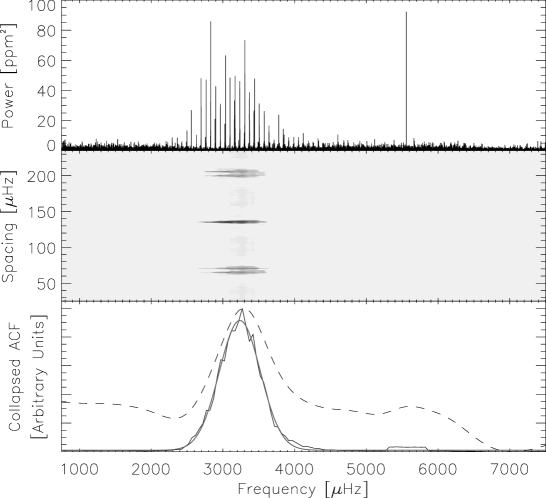
Figure 1: Procedure for locating the power excess using a 30 day subset of VIRGO photometry. Top panel: Background corrected power spectrum. Middle Panel: Autocorrelation as a function of frequency spacing and central frequency of the subset at which the correlation is evaluated. Dark colors are regions of high correlation. Bottom Panel: Collapsed ACF (black solid line) and smoothed power spectrum (dashed line). The grey solid line shows a Gaussian fit to the collapsed ACF.

More precisely, a vertical cut through the middle panel of Figure 1 at a given frequency is the ACF of the power spectrum subset centered at that frequency. In this example, the subset length chosen was 4$\Delta\nu$ ($\sim 540\,\mu$Hz). In applications where no estimate for $\Delta\nu$ is available, a range of up to three subset widths are applied and the one returning the highest S/N in the collapsed ACF is taken for the $\nu_{\rm max}$ estimate. As expected for this example, the ACF shows large values at multiples of half the large frequency spacing of the Sun ($\sim$ 68 $\mu$Hz), concentrated at frequencies around 3 mHz in the power spectrum. The collapsed ACF in the bottom panel is calculated by summing the middle panel vertically. For comparison, the dashed line shows the power spectrum smoothed with a Gaussian function with a FWHM of 4$\Delta\nu$.

An advantage of this technique over smoothing the power spectrum is that the collapsed ACF is strongly sensitive to the regularity of the peaks, rather than just their strengths. In other words, by applying an autocorrelation we use the information that peaks are expected to be regularly spaced, whereas this information is disregarded when smoothing the power. The single strong peak close to 6 mHz in the top panel of Figure 1, for example, is an artefact in the VIRGO photometry and produces a much more significant response in the smoothed spectrum than in the collapsed ACF. Figure 2 illustrates this further, using a power spectrum of a simulated Kepler star with low signal-to-noise. Compared to the smoothed power spectrum, the collapsed ACF shows a strong peak at the correct location of $\nu_{\rm max}$ and is clearly less sensitive to areas with white noise.

The shape of the power envelope in other stars can be very different than the Sun (e.g. for Procyon, see Arentoft et al. 2008) and hence might not be suitably modelled with a simple single Gaussian function. The collapsed ACF is less influenced by power asymmetries than a smoothed spectrum (see Figure 1, bottom panel), and an extension of the pipeline to include multiple Gaussians or different functions will be forthcoming. This will be of particular interest when analysing binaries in which both components show detectable power excess in the spectrum.

Figure 2: Same as Figure 1 but for a 1-month time series of a simulated Kepler star with low S/N. The vertical dotted line in the bottom panel is the true $\nu_{\rm max}$ value for this simulation. The large spacing was 88 $\mu$Hz.

3.2 Background modelling

Modelling of power due to stellar background is widely done using a sum of power laws initially proposed by Harvey (1985), with a revision of the power law exponent by Aigrain et al. (2003). Here, we use a mixture of the two versions that was originally suggested by Karoff (2008) and has the form

$$P(\nu)=P_{n}+\sum_{i=0}^{k}\frac{4\sigma_{i}^{2}\tau_{i}}{1+(2\pi\nu\tau_{i})^{2}+(2\pi\nu\tau_{i})^{4}}\>,$$ (1)

where $P_{n}$ is the white noise component, $k$ is the number of power laws used and $\sigma$ and $\tau$ are the rms intensity and timescale of granulation, respectively. The motivation behind this extended model is a more physically realistic interpretation of the stellar background. Instead of assuming a constant slope for the entire frequency range, it allows a shallower slope at low frequencies corresponding to turbulence (stellar activity) and steeper slopes at higher frequencies corresponding to granulation (Nordlund et al. 1997).

We determine $\sigma$ and $\tau$ using a least-squares fit to the power density spectrum. From a statistical point of view such an approach is questionable, since a raw power spectrum is not described by Gaussian statistics. We overcome this problem by smoothing the power spectrum using independent averages only (Garcia et al. 2009), which allows a determination of parameter uncertainties. Alternative methods such as a Bayesian approach using Markov-Chain Monte-Carlo simulations (T. Kallinger, private communication) could be used for more detailed studies of stellar granulation.

Regardless of the method of fitting, a pipeline relies on good initial conditions for a successful fit. To estimate such values, it is important to understand the rms intensity and, especially, the timescale of stellar granulation as a function of physical parameters. Based on numerical simulations of stellar surface convection, Freytag & Steffen (1997) initially suggested that the linear size of a granule $l$ is proportional to the pressure scale height on the stellar surface:

$$H_{p}^{\rm surf}=\frac{l}{\alpha}\>.$$ (2)

Here, $\alpha$ denotes the mixing length parameter. Assuming that the cells move proportional to the speed of sound $c_{s}$ (Svensson & Ludwig 2005), Kjeldsen & Bedding (in preparation) show that, under the further assumption of adiabacity and an ideal gas, the granulation timescale can be expressed as

$$\tau_{\rm gran}\propto\frac{H_{p}^{\rm surf}}{c_{s}}\propto\frac{L}{T_{\rm eff}^{3.5}M}\>.$$ (3)

According to Kjeldsen & Bedding (1995), this is inversely proportional to $\nu_{\rm max}$ and hence

$$\tau_{\rm gran}=\tau_{\rm gran,\odot}\frac{\nu_{\rm max,\odot}}{\nu_{\rm max}}\>.$$ (4)

This suggests that the timescale of granulation scales with the timescale of oscillations, which is plausible since both processes are tied to convection. Knowing $\nu_{\rm max}$ from the estimation performed in the previous section, granulation timescales can be scaled from the Sun without prior knowledge of stellar parameters.

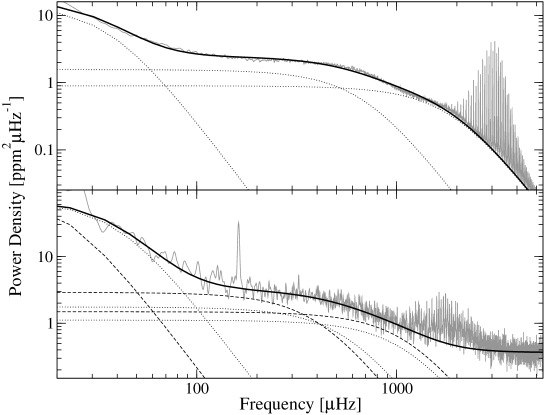
Figure 3: Power density spectra of a 9-year VIRGO time series (top panel) and a 60-day time series of HD49933 as observed by CoRoT (bottom panel). Dotted lines are the fitted individual power law components which, together with a white noise component (not shown), result in the final background model (thick solid lines). Dashed lines in the bottom panel show the initial guesses for the background fit using Equation 4. Note the differences in y-axis scaling for each panel.

We tested this scaling method on HD 49933, a star for which granulation and solar-like oscillations have been detected by CoRoT (Appourchaux et al. 2008). Figure 3 compares the power density spectrum of HD 49933 with the Sun, together with the individual power law components calculated using Equation 1. We assumed three components of stellar background in each spectrum: stellar activity at very low frequencies and two components due to different types of granulation. While the initial guesses for HD 49933 (dashed lines) using Equation 4 yield a satisfactory final fit (dotted and solid lines), it is evident that the background in this star is somewhat different from the scaled Sun. This result confirms that granulation signatures in hotter stars are quite different from the Sun, as found by Guenther et al. (2008) for a convection model of Procyon. We refer to Ludwig et al. (2009) for a detailed discussion of the granulation signal in HD 49933 in the context of hydrodynamical simulations.

Despite these differences for HD 49933, Equation (4) appears to be a satisfactory approximation to provide initial values for background fitting and hence we implemented it in the pipeline. After the background has been successfully fitted, the power spectrum is corrected by dividing through the background model.

3.3 Estimation of $\Delta\nu$

It is well known that the stochastic excitation and damping of solar-like oscillations causes series of peaks centred around the true frequency values in the power spectrum. To obtain a robust estimate of the average large frequency spacing, it is often helpful to divide the time series into subsets and co-add the corresponding power spectra, which leads to an average power spectrum with lower frequency resolution. In our pipeline, the background-corrected power spectrum is inverse-Fourier-transformed into the time-domain. The time series is then divided up into overlapping subsets (typically of 5 day length with a step size of 1 day) and power spectra of the individual subsets are co-added. This procedure forms a smoothed power spectrum. Figure 4 compares the original power spectrum with the background-corrected co-added power spectrum for a simulated Kepler star.

As a next step, we repeat the power excess determination described in Section 3.1 using the background corrected co-added power spectrum. Using this final value for $\nu_{\rm max}$, we estimate the expected spacing by using the tight correlation between $\nu_{\rm max}$ and $\Delta\nu$ discussed by Stello et al. (2009a)

$$\Delta\nu_{\rm exp}\propto\nu_{\rm max}^{0.8}\>.$$ (5)

Next, the autocorrelation of the power spectrum for the region $\nu_{\rm max}\pm 10\Delta\nu_{\rm exp}$ is calculated. Note that this width broadly agrees with the observed power excess in the Sun, and that we are at this stage only interested in deriving an average large frequency spacing over a large number of modes. Finally, we flag the five highest peaks in the autocorrelation, and fit a Gaussian function to the peak among the five which is closest to $\Delta\nu_{\rm exp}$, yielding the final determination of $\Delta\nu$. Figure 5 shows a $\Delta\nu$ measurement of a simulated Kepler star for which the correct spacing does not correspond to the highest peak in the autocorrelation.

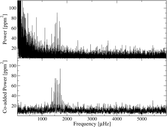
Figure 4: Top panel: Original power spectrum of a simulated Kepler star with a time base of one month. Bottom panel: Background-corrected and co-added power spectrum of the same star.

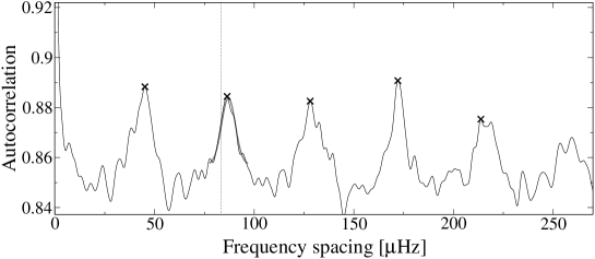
Figure 5: ACF of the background-corrected co-added power spectrum of a simulated Kepler star. Black crosses mark the five highest peaks. The grey line is a fit to the peak among the five which is closest to $\Delta\nu_{\rm exp}$ (vertical dotted line).

3.4 Uncertainties in $\nu_{\rm max}$ and $\Delta\nu$

A crucial part of an automated pipeline is the ability to interpret the quality (or credibility) of the returned values. However, since we determine $\nu_{\rm max}$ and $\Delta\nu$ using least-squares fits to autocorrelation functions, determining reliable uncertainties is not straight forward. As pointed out by Chaplin et al. (2008b), the formal uncertainties of such fits are strongly underestimated since the datapoints to which functions are fitted are highly correlated, and no proper weights (or uncertainties) can be assigned to individual datapoints. Additionally, the stochastic nature of solar-like oscillations introduces an intrinsic scatter of our measured $\nu_{\rm max}$ and $\Delta\nu$ values.

To overcome this, we followed the approach of Chaplin et al. (2007) and performed simulations by producing synthetic time series. The inputs for each simulation were solar frequencies covering roughly twelve orders of $\ell=0-2$ modes taken from BiSON observations (Broomhall et al. 2009). We modelled the amplitudes using a solar envelope derived from smoothing a power spectrum calculated from a 30-day subset of VIRGO photometry. For simplicity, we assumed that all modes are intrinsically equally strong, but accounted for different spatial responses of $\ell=0-2$ modes according to Kjeldsen et al. (2008a). We simulated the stochastic excitation and damping using the method of Chaplin et al. (1997), with a frequency independent mode lifetime of three days (i.e. solar). Each time series consisted of the same sampling and time base as the simulated asteroFLAG stars, and white noise was added to each synthetic time series.

We performed simulations with different input amplitudes and frequencies to resemble a range of stellar evolutionary states, and with different S/N corresponding to a variety of stellar magnitudes. We made 100 realizations, including stochastic excitation and white noise for each set of input parameters. The resulting light curves were then analysed by the pipeline, and the standard deviations of the determined values for $\nu_{\rm max}$ and $\Delta\nu$ were taken as the true uncertainties.

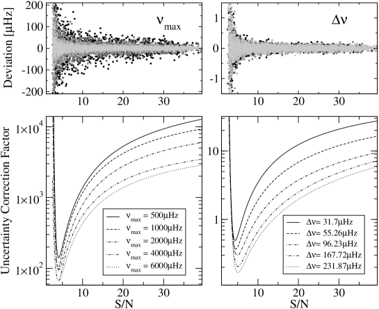
Figure 6: Top panels: Scatter of $\nu_{\rm max}$ (left) and $\Delta\nu$ (right) from simulations as a function of S/N. Darker colours correspond to higher input values of $\nu_{\rm max}$ and $\Delta\nu$, respectively. Bottom panels: Correction factors for formal uncertainties as a function of S/N and input value.

The results of the simulations are shown in Figure 6. The top panels show the scatter in $\nu_{\rm max}$ and $\Delta\nu$ as a function of S/N. We see that the scatter of $\nu_{\rm max}$ is greater for higher values of $\nu_{\rm max}$ (darker symbols), while the scatter in $\Delta\nu$ is almost independent of $\Delta\nu$. This is expected, since the power excess hump used to determine $\nu_{\rm max}$ becomes broader for higher input values of $\nu_{\rm max}$ and hence the absolute deviation increases. On the other hand, the peak in the autocorrelation used to determine $\Delta\nu$ will remain about the same because it is determined by the frequency resolution and mode lifetime, which are the same for all simulations. We note that the scatter reaches a constant level for high S/N, and the maximum precision with which $\nu_{\rm max}$ and $\Delta\nu$ can be determined are $\sim$10 $\mu$Hz and $\sim$0.1 $\mu$Hz, respectively. The latter value is in good agreement with the uncertainties reported in the first asteroFLAG exercise (Chaplin et al. 2008b).

The ratio between these values and the formal uncertainties as determined by the least-squares fit give a look up table of correction factors which we use to convert the formal uncertainties into more realistic values. To obtain smoothly varying correction factors, we fitted power laws to the results of the simulations. These are shown in the bottom panels of Figure 6. As expected, the factors increase for higher S/N, i.e. the least squares fit underestimates uncertainties more for higher signal because the correlation between fitted points is higher. Towards the detection limit at low S/N, this trend quickly reverses and formal uncertainties must be scaled with high factors to accommodate the large uncertainty due to high noise levels. We note that at S/N values around 10 and lower, the $\Delta\nu$ uncertainties determined by the least-squares fit are in fact overestimated, with correction factors $<$ 1. Considering that our simulations are simplified compared to real data and therefore the scatter at low S/N values is likely underestimated, we disregard this effect and do not downscale formal uncertainties.

We note that the uncertainty correction presented here will also be applicable to real Kepler stars, with slight adaptations for different sampling and observing lengths. In preparation for this, we test our uncertainties using simulated Kepler stars, which will be presented in the next section.

4 Application to simulated Kepler observations

We applied the pipeline, as described in the previous section, to 1936 simulated Kepler stars discussed in Section 2. To verify the values returned by the pipeline, we calculated “true” values of $\nu_{\rm max}$ and $\Delta\nu$ as follows: Using the stellar mass, luminosity and effective temperature of the input model, we calculated $\nu_{\rm max,true}$ using the scaling relation by Kjeldsen & Bedding (1995). To determine $\Delta\nu_{\rm true}$, we first determine the input model frequency closest to $\nu_{\rm max,true}$. We then fitted a linear regression to ten orders of the same degree around the frequency of maximum power, and used the slope to estimate the frequency spacing (Kjeldsen et al. 2008b). This was done separately for modes of $\ell=0-2$, and the final value of $\Delta\nu_{\rm true}$ is a weighted mean of the three spacings, with weights corresponding to the spatial responses as given by Kjeldsen et al. (2008a). Note that for more evolved stars ($\Delta\nu<70\,\mu$Hz), no reliable model frequencies were available and hence the scaling relation by Kjeldsen & Bedding (1995) was used to calculate $\Delta\nu_{\rm true}$.

To investigate systematic effects in our uncertainty simulations from section 3.4, we repeated these simulations for noise-free realizations and compared $\nu_{\rm max}$ and $\Delta\nu$ returned by the pipeline to $\nu_{\rm max,true}$ and $\Delta\nu_{\rm true}$ for these simulations. We found that on average the determined $\nu_{\rm max}$ values are $\sim$ 1% higher and that the determined $\Delta\nu$ values are $\sim$ 0.05 % lower than the input values. Both effects are easily understood: In our uncertainty simulations, as well as the Kepler simulations, a solar oscillation profile was assumed. While the amplitudes in this profile have positive asymmetry, the large spacings increase towards higher frequencies. The collapsed ACF used to determine $\nu_{\rm max}$ is sensitive to regular peak spacings, and hence overestimates $\nu_{\rm max}$ compared to our definition of $\nu_{\rm max,true}$, which is not equal to the center of the solar envelope. The single ACF used to measure $\Delta\nu$ is influenced by the peak power, and hence underestimates $\Delta\nu$ compared to our definition of $\Delta\nu_{\rm true}$, which is the mean spacing across the envelope independent of amplitude. For this application, we account for both effects by multiplying the measured $\nu_{\rm max}$ values by 0.99 and the measured $\Delta\nu$ values by 1.0005.

We now proceed to the main results by comparing the measured values of the 1936 Kepler stars with the true values. Figures 7 and 8 display the differences between the true values (as defined above) to the quantities measured by the pipeline for $\nu_{\rm max}$ and $\Delta\nu$, respectively. In this comparison we have eliminated all stars with relative uncertainties greater than 10%. Furthermore, we disregard extreme outliers by considering only measurements for which the absolute difference of $\Delta\nu$ and $\Delta\nu_{\rm exp}$ is lower than 0.1 $\Delta\nu_{\rm exp}$, and the absolute difference of $\nu_{\rm max}$ and $\nu_{\rm max,exp}$ is lower than 0.5 $\nu_{\rm max,exp}$. $\nu_{\rm max,exp}$ is calculated using the scaling relation by Kjeldsen & Bedding (1995) with the Kepler Input Catalog parameters for these stars. Of the entire sample, 52% of the $\nu_{\rm max}$ and 48% of the $\Delta\nu$ measurements fulfill these criteria.

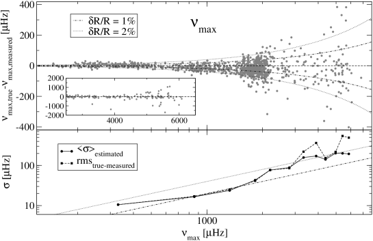
Figure 7: Top panel: Differences between true and measured values for $\nu_{\rm max}$ for all measurements with an uncertainty precision lower than 10%. The inset shows the comparisons on a larger scale to display measurements with larger deviations. Bottom panel: Mean estimated uncertainties of the measurements (solid line) compared to the actual scatter of measurements and true values (dashed line). In both panels, the dashed-dotted and dotted lines display uncertainty limits necessary to constrain stellar radii to 1% and 2%, respectively.

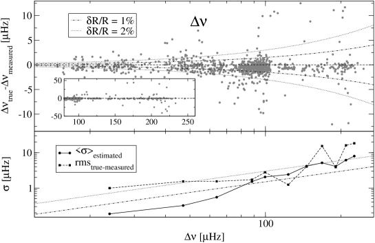
Figure 8: Same as Figure 7 but for $\Delta\nu$.

The largely symmetric distributions for both $\nu_{\rm max}$ and $\Delta\nu$ in the top panels of Figures 7 and 8 suggest that systematic effects caused by the methods of the pipeline have been mostly removed or corrected. We suspect that the slight negative trend for high values of $\Delta\nu$ is due to the fact that $\Delta\nu_{\rm true}$ is calculated based on a fixed number of model frequencies, which underestimates $\Delta\nu_{\rm true}$ compared to simulated Kepler stars where less low-frequency modes might be visible. As discussed in section 3.4, the scatter in $\nu_{\rm max}$ gets considerably larger as the power excess shifts to higher frequencies and the oscillation amplitudes become smaller. The bottom panels show the mean uncertainties and the rms of measured minus true values. In both cases, the curves are for the most part overlapping. The exception are low values of $\Delta\nu$ for which the uncertainties still seem considerably underestimated. We suspect that this is partially connected to the fact that for these stars $\Delta\nu_{\rm true}$ was calculated using a scaling relation rather than the actual model frequencies (see above).

An important application of asteroseismology within the Kepler mission will be to determine radii of of exoplanet host stars. As noted by Chaplin et al. (2008b), a radius determination to a precision of 1% requires a relative uncertainty of 0.15 % on the large frequency spacing. Formally, this corresponds to a 2% relative uncertainty on $\nu_{\rm max}$. These precisions are indicated in Figures 7 and 8 by dashed-dotted lines. We also show the precisions required for a more pessimistic radius precision of 2% (dotted lines). The scatter of the measured values and the mean uncertainties shows that the 1% limit should be achievable for a considerable number of stars up to $\Delta\nu\sim$ 100 $\mu$Hz and $\nu_{\rm max}\sim$ 2000 $\mu$Hz, and even higher values if the criterion is relaxed to a radius precision of 2% or 3%. These results therefore indicate an optimistic outlook for the automated analysis of Kepler asteroseismology stars, despite the fact that the time base of the initial survey will only be about 30 days.

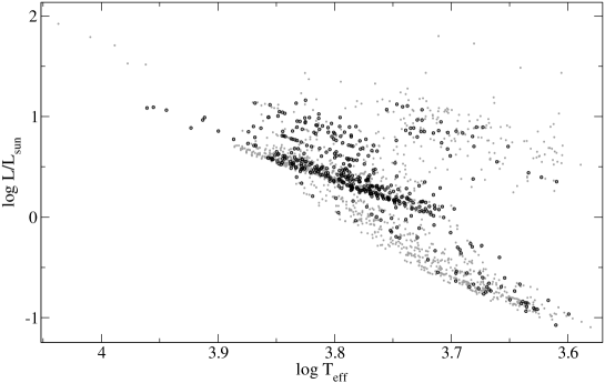
Figure 9: H-R diagram of all 1936 stars in the test sample based on the model parameters. Black circles show stars for which the pipeline returned correct large frequency spacings precise enough to determine the stellar radius to a precision of 1%.

To analyse these results in terms of stellar evolution, Figure 9 shows a H-R diagram based on the model parameters of all 1936 sample stars. The majority of the test sample was made up of main sequence and sub-giant stars. As expected, a large part of the best $\Delta\nu$ determinations (with uncertainties allowing a radius determination to 1% precision) were made in stars with relatively high luminosities. The relative lack of detections for the evolved sub-giants compared to the rest of the sample points to a problem of our pipeline with handling signal at the very low frequencies. Quite surprisingly, the results also indicate that precise $\Delta\nu$ determinations will be possible for a number of cool, low-mass main-sequence stars (which represent the datapoints at very high $\nu_{\rm max}$ and $\Delta\nu$ in Figures 7 and 8).

5 Summary & Conclusions

We have described an automated analysis pipeline to extract global oscillation parameters for a large number of stars. We demonstrated that the use of a collapsed autocorrelation function is a sensitive tool to find the location of excess power. We further showed that a determination of $\nu_{\rm max}$ can be used to scale granulation timescales in order to model the background contribution in the power spectrum. To obtain robust uncertainty estimates on $\nu_{\rm max}$ and $\Delta\nu$, we have performed realistic simulations of solar-like oscillations as a function of S/N and $\nu_{\rm max}$, and derive correction factors which are necessary to convert least-squares uncertainties derived from correlated data to realistic uncertainties. Our simulations indicate that for a one-month time series with one-minute sampling, the maximum precision with which $\nu_{\rm max}$ and $\Delta\nu$ can be determined are $\sim$10 $\mu$Hz and $\sim$0.1 $\mu$Hz, respectively.

The automated pipeline was applied to a sample of 1936 simulated stars representing targets of the Kepler asteroseismic survey phase. We show that our scaled uncertainties are reliable for all values of $\nu_{\rm max}$, but seem to be significantly underestimated for $\Delta\nu<50\mu$Hz. While we suspect that this is mostly due to the fact that $\Delta\nu_{\rm true}$ could not be calculated accurately from model frequencies for evolved stars, the results show that in general some modifications of the code are needed for processing stars that pulsate at low frequencies ($<$ 500 $\mu$Hz). The further development of the pipeline, in particular with respect to the background modelling, will focus on this adaptation to process red giant stars.

The comparison of real and measured values showed that in 70% and 60% of all cases, $\nu_{\rm max}$ and $\Delta\nu$ were recovered within 10 % of the true value, respectively. Using the estimated uncertainties to eliminate measurements with too large uncertainties and disregarding extreme outliers, these numbers drop to roughly 50%. The scatter of the measured values around the input values and the mean uncertainties agrees well for this sample, and indicate that for at least 20% of the stars $\Delta\nu$ can be determined with a precision sufficiently high to infer stellar radii to 1% accuracy. Plotting these stars in an HR diagram suggests that their distribution is quite diverse, including low-mass main sequence stars as well as evolved sub-giants.